Increased seawater viscosity, Phaeocystis globosa spring bloom and Temora longicornis feeding and swimming behaviours

HAL Id: hal-00481287

https://hal.archives-ouvertes.fr/hal-00481287

Submitted on 10 May 2021

HAL is a multi-disciplinary open access

archive for the deposit and dissemination of

sci-entific research documents, whether they are

pub-lished or not. The documents may come from

teaching and research institutions in France or

abroad, or from public or private research centers.

L’archive ouverte pluridisciplinaire HAL, est

destinée au dépôt et à la diffusion de documents

scientifiques de niveau recherche, publiés ou non,

émanant des établissements d’enseignement et de

recherche français ou étrangers, des laboratoires

publics ou privés.

Distributed under a Creative Commons Attribution| 4.0 International License

bloom and Temora longicornis feeding and swimming

behaviours

Laurent Seuront, Dorothée Vincent

To cite this version:

Laurent Seuront, Dorothée Vincent. Increased seawater viscosity, Phaeocystis globosa spring bloom

and Temora longicornis feeding and swimming behaviours. Marine Ecology Progress Series, Inter

Research, 2008, 2008, pp.131-145. �hal-00481287�

INTRODUCTION

The cosmopolitan phytoplankton genus Phaeocystis

(Prymnesiophyceae) constitutes a key organism in dri-ving global geochemical cycles, climate regulation and fisheries yield; for example see Schoemann et al. (2005) for a review. Of particular importance is the existence of a complex polymorphic life cycle exhibit-ing phase alternation between solitary flagellated cells and gelatinous colonies (Rousseau et al. 1994). Even if

blooms of solitary cells occur, most large blooms are dominated by colonies (Peperzak et al. 2000), leading to the widely acknowledged belief that the success of

Phaeocystis is largely a consequence of its ability to

form gel-like colonies (Schoemann et al. 2005). Colony formation seems to be an evolutionary ad-vantage as colonies are apparently resistant to viral infection (Bratbak et al. 1998). Recent empirical evi-dence (Tang 2003) confirmed the long-held belief that

Phaeocystis sp. colony formation is a defence strategy,

© Inter-Research 2008 · www.int-res.com *Email: laurent.seuront@flinders.edu.au

Increased seawater viscosity,

Phaeocystis globosa

spring bloom and

Temora longicornis feeding and

swimming behaviours

Laurent Seuront

*, Dorothée Vincent

1_{School of Biological Sciences, Flinders University, GPO Box 2100, Adelaide, South Australia 5001, Australia} 2_{South Australian Research and Development Institute, Aquatic Sciences, West Beach, South Australia 5022, Australia} 3_{Laboratoire d’Océanologie et de Géosciences, Centre National de la Recherche Scientifique (CNRS) UMR 8187, Maison de}

la Recherche en Environnement Naturel, Université du Littoral-Côte d’Opale, 32 avenue Foch, 62930 Wimereux, France

ABSTRACT: The suggested influence of increased seawater viscosity on the feeding and swimming behaviours of adult females of the calanoid copepod Temora longicornis was investigated during a Phaeocystis globosa spring bloom in the coastal waters of the eastern English Channel. Adult female

gut contents did not exhibit any significant correlation with chlorophyll concentration or seawater excess viscosity over the course of the bloom. Instead, the highest gut contents were observed when the seawater viscosity was maximum (up to 4.6 centipoise [cP]), after a 5-fold decrease in chlorophyll concentration related to the formation of foam. This demonstrates that even high viscosity did not mechanically hamper zooplankton grazing. Gut contents were controlled by the taxonomic availabil-ity rather than the quantitative availabilavailabil-ity of phytoplankton-based food. This is consistent with the observed sustained egg production rates despite drastic changes in the composition of protist resource over the course of the bloom. Before and after the bloom (in the absence of P. globosa), T. longicornis exhibited similar swimming paths characterized by their large spatial extent and low

curviness. In contrast, during the bloom their movements were spatially more localised, significantly slower and more convoluted. This behaviour is suggested as an adaptive strategy to optimise forag-ing activity durforag-ing P. globosa blooms, which have been recently shown to generate high level of

phytoplankton patchiness.

KEY WORDS: Zooplankton · Motility · Behaviour · Viscosity · Phaeocystis · Temora longicornis ·

Fractal

as millimetre-scale (Peperzak et al. 2000) to centi-metre-scale (Chen et al. 2002) colonies create a size-mismatch problem for small grazers (Weisse et al. 1994). Another consequence of the formation of gel-like Phaeocystis colonies is the potential effects of

phytoplankton-derived polymeric materials on seawa-ter properties. More specifically, a positive correlation has been found between seawater viscosity and chlorophyll a (chl a) concentration during Phaeocystis

blooms in the German Bight and the North Sea (Jenk-inson & Biddanda 1995). These early results have been amplified by studies conducted over the course of a

P. globosa bloom in the eastern English Channel that

showed the existence of positive and negative correla-tions between chlorophyll concentration and seawater viscosity before and after foam formation respectively (Seuront et al. 2006, 2007). This suggests that seawater rheological properties are mainly driven by extracellu-lar materials associated with colony formation and maintenance rather than by cell composition and standing stock (Seuront et al. 2006). The resistance of

Phaeocystis colonies to mesozooplankton grazing has

also been attributed to a mechanical hindrance due to increased viscosity (Weisse et al. 1994). However, the increase in seawater viscosity during Phaeocystis sp.

(Jenkinson & Biddanda 1995) and P. globosa (Seuront

et al. 2006, 2007) blooms has barely been investigated and its subsequent potential effects on zooplankton trophodynamics have never been demonstrated or investigated (Schoemann et al. 2005).

In the coastal zone of the eastern English Channel, blooms of the colony-forming Phaeocystis globosa are

a recurring phenomenon and often coincide with max-imal abundance of the calanoid copepod Temora longi-cornis (Fransz et al. 1992). P. globosa dominates the

phytoplankton community, contributing over 73% of the total phytoplankton abundance and reaching max-imum abundance of ca. 6 × 106 _{cells l}–1_{(Seuront et al.}

2006). While T. longicornis is able to remove up to 49%

of the daily primary production (Dam & Peterson 1993), grazing studies on P. globosa single cells are still

con-troversial (see Nejstgaard et al. 2007 for a review). Rel-atively high (Koski et al. 2005) and low (Cotonnec et al. 2001) feeding rates have been reported for T. longicor-nis grazing on P. globosa. P. globosa often represents a

poor food source for zooplankton production and growth (Klein Breteler & Koski 2003). This suggests that copepods switch to alternative food sources during the bloom (e.g. ciliates and dinoflagellates; Gasparini et al. 2000, Koski et al. 2005). Since swimming and feeding behaviours are intrinsically linked in most calanoid copepods, we studied the swimming and feeding responses of T. longicornis before, during and

after a P. globosa bloom, to reveal whether grazing by T. longicornis adult females is affected by

biologically-induced modification of seawater viscosity and poten-tially related to the protist cell composition and stand-ing stock.

MATERIALS AND METHODS

Field site and sampling strategy. The sampling

site was located at the inshore station (50° 40’ 75’’ N, 1° 31’ 17’’ E) of the Service d’Observation du Milieu Lit-toral (SOMLIT) network in the coastal waters of the eastern English Channel. The eastern English Channel is characterized by its megatidal range of between 3 and 9 m. Tides are characterized by a residual circu-lation parallel to the coast, with nearshore coastal waters drifting from the English Channel into the North Sea. Coastal waters are influenced by freshwa-ter run-off from the Seine estuary to the Strait of Dover. This ‘Coastal Flow’ is separated from offshore waters by a tidally maintained frontal area. The inshore water mass is characterized by its low salinity, turbidity, phytoplankton richness and productivity, when com-pared with the oceanic offshore waters. The sampling site was chosen as the physical and hydrological prop-erties encountered here are representative of the inshore water masses of the eastern English Channel. Sampling was conducted weekly at high tide before, during and after the Phaeocystis globosa bloom in the

eastern English Channel from February to June 2004. Water temperature (°C) and salinity (PSU) profiles from surface to bottom were measured using a Seabird SBE 19 or Seabird SBE 25 Sealogger CTD at each sam-pling date. The maximum depth never exceeded 25 m. Water samples were taken from sub-surface waters using 5 l Niskin bottles. Chl a concentrations and

sea-water viscosity were systematically estimated from the same water samples. The composition and standing stock of auto-, hetero- and mixotrophic protists were investigated from 1 l sub-surface samples.

At each sampling date, surface seawater (40 l) was collected and stored in a polycarbonate carboy for further use in the laboratory during the behavioural experiments. Zooplankton were collected with a WP2 net (200 μm mesh size) fitted with a 1 l filtering cod-end hauled horizontally (<1 m s–1, mean duration less than 10 min) through the upper 5 m of the water col-umn. Aliquots of this sample were immediately deep-frozen in liquid nitrogen to minimize faecal pellet production (Saiz et al. 1992) and kept frozen at –80°C in the dark until gut content analysis. Specimens were also gently diluted in 30 l isotherm tanks using in situ seawater and transported within 1 h to the

labo-ratory. Temora longicornis adult females were then

immediately sorted by pipette under a dissecting microscope and acclimated for 2 h in a 2 l beaker

containing fresh in situ seawater prior to the

behav-ioural experiments.

All the parameters considered here were investi-gated from sub-surface samples (1) because previous experiments conducted from the same inshore sam-pling site always showed the water column to be verti-cally homogenized (e.g. Seuront et al. 2006), and (2) to avoid any confusing interpretation that could result from benthic and tychoplanktonic phytoplankton resuspended in the bottom layer of the water column, as their proportion is highly variable at different time scales and strongly depends on the energy dissipation rates of the environment (e.g. spring/neap tide cycle, season, wind stress).

Chlorophyll analysis. Chlorophyll concentrations

were estimated from 500 ml seawater samples. Sam-ples were vacuum filtered on Whatman GF/F glass fi-bre filters (porosity 0.45 μm). Chlorophyllous pigments were extracted by direct immersion of the filters in 5 ml of 100% N,N-dimethylformamide, and actual extrac-tions were made in the dark at –20°C for 12 h. Con-centrations of chl a in the extracts were determined

following Strickland & Parsons (1972) using a Turner 450 fluorometer previously calibrated with chl a

extracted from Anacystis nidulans (Sigma Chemicals,

St Louis).

Protist community composition. For micro- and

nanoplankton analyses 1 l samples were preserved in the field with acid Lugol’s iodine solution (2% final concentration) and stored in the dark at 4°C. Enumer-ation was carried out using the Utermöhl (1958) set-tling method within a month after collection (typically

7 to 21 d), a time period that does not lead to any sig-nificant changes in Phaeocystis globosa colony size

and abundance after Lugol’s preservation (p > 0.05, n = 357; L. Seuront unpubl. data). Sub-samples of 10 to 20 ml in sizewere allowed to settle for 24 h in Hydro-bios counting chambers and settled slides were observed by inverted microscopy (Olympus, 200× and 400× magnification). Autotrophic protists were identi-fied according to Sournia (1986), Ricard (1987), Paul-mier (1997) and Tomas (1997). Cells were measured with an eyepiece micrometer and corresponding bio-volumes (μm3_{) were calculated by relating the shape of}

organisms to a standard geometric form of known vol-ume. Cell biovolumes were converted to carbon bio-mass following Menden-Deuer & Lessard (2000) and Menden-Deuer et al. (2001).

The first appearance of Phaeocystis globosa colonies,

their size (total length and width) and shape were de-termined throughout the survey according to Rousseau et al. (1990). Small colonies (≤200 μm maximum dimen-sion) were often spherical, medium colonies (200 to 350 μm) were either spherical or ellipsoid, and large colonies (> 350 μm) were either ellipsoid or typically ghost colonies (i.e. large flat areas of skin-like matrix). The proportion of ghost colonies markedly increased over the course of the bloom (Table 1). The number of cells per colony was determined by inverted microscopy under contrast phase illumination, i.e. cells appeared brighter than their background. For large ghost, small spherical and ellipsoid colonies, direct enumeration was carried out by counting the number of cells within each colony with a 20× Plan Ph1 0.50NA objective. For large Table 1. Time course of measured seawater viscosity ηm(cP), physically controlled component of seawater viscosity ηT,S(cP) esti-mated in the laboratory from viscosity measurements conducted on filtered (0.20 μm mesh size), and seawater excess viscosity η (%); length (μm), width (μm), shape (S = spherical, E = ellipsoid, G = ghost colony [large flat areas of skin-like matrix]) of Phaeo-cystis globosa colonies in order of importance; range of P. globosa cells per colony; and mean prosome length (PL) of Temora

longicornis adult females (mm). The numbers in parentheses are SD values

Bloom period Date Seawater viscosity P. globosa colonies T. longicornis

ηm(cP) ηT,S(cP) η (%) Length (μm) Width (μm) Shape cells colony–1 PL (mm)

Pre-bloom 16 Feb 2004 – – – – – – – – –

(B0) 2 Mar 2004 1.63 1.49 9.2 – – – – 0.96 (0.04)

10 Mar 2004 1.71 1.56 9.8 – – – – 0.98 (0.06)

Bloom/no foam 22 Mar 2004 2.04 1.57 29.6 – – – – 0.98 (0.02)

(B1) 29 Mar 2004 2.93 1.49 96.8 70–627 30–275 S, E 8–259 0.99 (0.09) 8 Apr 2004 3.68 1.41 161.2 120–570 60–315 S, E 15–144 0.96 (0.09) 13 Apr 2004 2.92 1.40 108.9 60–374 60–180 S, E, G 16 –127 0.99 (0.03) 20 Apr 2004 3.45 1.41 144.6 60–784 40–394 G, S, E 9–194 0.98 (0.01) 30 Apr 2004 3.80 1.38 175.7 90–1060 90–955 G, S, E 15–566 1.00 (0.02) Bloom/foam 7 May 2004 3.13 1.37 128.2 – – – – 1.03 (0.03) (B2) 18 May 2004 4.58 1.32 247.1 200–1146 80–1146 G 40–1201 0.98 (0.07) 25 May 2004 4.17 1.29 223.0 265–1040 40–765 G 25–55 1.04 (0.06) 3 Jun 2004 2.09 1.25 67.4 – – – – 0.95 (0.04) Post-bloom 15 Jun 2004 1.36 1.20 13.2 – – – – 1.03 (0.02) (B3) 8 Jul 2004 1.23 1.15 7.3 – – – – 0.99 (0.02)

spherical and ellipsoid colonies, cell counting was car-ried out by sequentially focusing through each colony with a 10× Plan Ph1 0.25NA objective . While the enu-meration of cells in large colonies may be tedious and problematic (Verity et al. 2007), the linear regressions found between number of cells per colony and the colony volume did not significantly differ between colony types (analysis of covariance, p > 0.05). This re-sults in the number of cells per colony, N, being highly

significantly correlated (p < 0.001, n = 80) with colony volume, V (mm3_{), as logN = 0.33logV + 2.53. In addition,}

a close examination of the residuals of this regression did not exhibit any significant local slope that might have been indicative of a bias related to an underestimation of cell number in large colonies. The contribution of Phaeo-cystis to carbon biomass was estimated using the

conver-sion factor of 122 pgC cell–1_{defined by van Rijssel et al.}

(1997), which included colonial mucus. Due to their het-erotrophic status, some of the dinoflagellates counted during the survey (Gyrodinium sp.) were analysed

sep-arately. Since Lugol’s preservation does not allow unam-biguous identification of ciliates, ciliate enumeration considered total ciliates and mainly included oligo-trichous ciliates (30 to 40 μm length) and large tintinnids (> 60 μm; Acineta sp.). Ciliate carbon biomass was

calcu-lated from cell biovolumes (estimated as described pre-viously) using a volume-to-carbon conversion factor of 0.19 pgC μm– 3_{that accounts for cell shrinkage (Putt &}

Stoecker 1989). No taxonomic data were available on May 7.

Seawater excess viscosity measurements. Viscosity

measurements were conducted with a portable Visco-Lab400 viscometer (Cambridge Applied Systems) fol-lowing Seuront et al. (2006, 2007) from 10 ml water samples stored in the dark in a bucket maintained at

in situ temperature. Viscosity was estimated in

tripli-cate from 2 to 3 ml water samples poured into a small chamber, where a low mass stainless steel piston is magnetically forced back and forth with a 230 μm pis-ton-cylinder gap size. Because the force driving the piston is constant, the time required for the piston to move back and forth into the measurement chamber is proportional to the viscosity of the fluid. The more vis-cous the fluid the longer it will take the piston to move through the chamber, and vice versa. As viscosity is influenced by temperature and salinity, the measured viscosity ηmin centipoise (cP) is the sum of a physically

controlled viscosity component ηT,S(cP) and a

biologi-cally controlled viscosity component ηBio(cP), i.e.:

ηm = ηT,S+ ηBio (1)

To ensure that the viscosity component ηBio

corre-sponds to extra-colonial polymeric materials contained in the bulk phase seawater, and not to intra-colonial materials released during the measurement through

the disruption of colonies in the chamber of the visco-meter, viscosity measurements were conducted on sub-samples where colonies were removed using a Pasteur pipette under a dissecting microscope (100× magnification). The physically controlled component ηT,S was estimated in the laboratory from viscosity

measurements conducted on filtered (0.20 μm mesh size) seawater from the same samples. The biologically induced excess viscosity, ηBio, was subsequently

esti-mated with confidence from each water sample as ηBio= ηm– ηT,S. The related relative excess viscosity η

is, thus, given by (Seuront et al. 2006, 2007):

η = (ηm– ηT,S) / ηT,S (2)

Before each viscosity measurement, temperature and salinity of the seawater sample were simultane-ously measured using a Hydrolab probe. Between each viscosity measurement, the viscometer chamber was carefully rinsed with deionised water and bulk phase seawater filtered through 0.2 μm pore size filters to avoid any potential dilution of the next sample. To avoid any bias related to temperature changes, all vis-cosity measurements were conducted in a tempera-ture-controlled room set up at in situ temperature.

Zooplankton gut content.In the laboratory, 5

Temo-ra longicornis adult females were picked from the

frozen samples under a binocular microscope and cool light. Organisms were rinsed with filtered seawater, transferred and ground with a tissue homogenizer in 5 ml of 100% N,N-dimethylformamide, and chloro-phyllous pigments were then extracted in the dark at –20°C for 12 h. Gut content was analysed fluoro-metrically (Mackas & Bohrer 1976), and gut fluores-cence readings were taken before and after acidifica-tion with 50 μl of 10% HCl using a Turner 450 fluorometer. Gut contents (GC hereafter) were con-verted to equivalent chlorophyll ingested following Dagg & Wyman (1983).

Video setup and behavioural observations.For each

date, 5 behavioural experiments were done with

Temora longicornis adult females in a temperature

controlled dark room (20°C) in a 2 l (20 × 20 × 5 cm) Plexiglas behavioural container described previously by Seuront (2006). Prior to each experiment, an indi-vidual was selected from the female stock, transferred to the experimental filming setup, which was filled with fresh in situ seawater, and allowed to acclimatise

for 15 min. The 2D trajectory of the copepod was recorded at a rate of 25 frame s–1_{using a infrared}

digi-tal camera (DV Sony DCR-PC120E) facing the front view of the experimental container. Two arrays of 72 infrared light emitting diodes (LEDs), each mounted on a printed circuit board about 9.3 cm long and 4.9 cm wide connected to a 12 V DC power supply, provided the only light source. All experiments were conducted

in the dark and at night to avoid any potential behav-ioural artefact related to the diel light cycle.

Each female was recorded swimming for 60 min, after which valid video clips were identified for analy-sis. Valid video clips consisted of pathways in which the animals were swimming freely, at least 2 body lengths away from any chamber walls or the surface of the water. Between 6 and 30 swimming paths were considered for each sampling date and female. Dura-tion of individual observaDura-tions varied, and swimming path durations ranged from 15 s to 2 min. Although we considered copepods filmed in one 2D aquarium only, we ensured that the behaviour was representative of the species for each experiment by qualitatively observing the general swimming behaviour of females

Temora longicornis in other 3D aquaria.

Before each experiment, 500 ml of the seawater used for the behavioural experiment were vacuum filtered on Whatman GF/F glass-fibre filters for chlorophyll concentration measurements. Before and after each experiment, triplicate 3 ml seawater samples were measured for viscosity. No significant differences were found between chlorophyll concentrations estimated from in situ and experimental water

(Wilcoxon-Mann-Whitney test, p > 0.05). Also, no significant differences were found between the seawater excess viscosity esti-mated from in situ water samples and the experimental

water from both before and after each behavioural experiment (Kruskal-Wallis test, p > 0.05). At the end of the experiment, individuals were sorted by pipette and preserved in formalin for size determination.

Image analysis and behavioural analysis. Selected

video clips were captured (DVgate Plus, 25 frames s–1₎

as MPEG movies and converted into QuickTime™ movies (QuickTime Pro), after which the x and y

coor-dinates of swim paths were automatically extracted and subsequently combined into a 2D picture using LabTrack software (DiMedia, Kvistgård, Denmark). The time step was always 0.04 s, and output sequences of (x, y) coordinates were subsequently used to

charac-terise the motility.

Swimming paths may be characterised by a variety of measures, including for example path length (the total distance travelled, or gross displacement), move length (the distance travelled between consecutive points in time), move duration (the time interval be-tween successive locations), turning angle (the differ-ence in direction between 2 successive moves), turning rate (the turning angle divided by move duration) and net displacement (the linear distance between starting and ending point); see Seuront et al. (2004) for a review. As discussed elsewhere (Seuront et al. 2004), all of these metrics are implicitly a function of their measurement scale, and there is no single scale at which swimming paths can be unambiguously

des-cribed. This is not the case for fractal dimensions, which are scale-independent. However, because frac-tal dimensions have seldom been used in zooplankton behavioural studies (see Seuront et al. 2004 for a re-view), more common behavioural measures were also used to provide a reference framework for the reader to make comparisons with previous studies having similar temporal resolution.

Swimming activity index: The level of activity of a

copepod is estimated as the percentage of time allo-cated to swimming. The activity index Ai is then

defined as:

(3)

where ttrackand tswimare the duration of a swimming path and the time a copepod spent swimming, respec-tively.

Swimming speed: The distance dt(mm) between 2

points in a 2-dimensional space was computed from the x and y coordinates as:

(4) where (xt, yt) and (xt+1, yt+1) are the positions of a

cope-pod at time t and t + 1, respectively. The swimming

speeds over consecutive tracking intervals (i.e. 40 ms) were subsequently estimated as:

(5) where ƒ is the sampling rate of the camera, i.e. ƒ = 25 frames s–1_{. Average swimming speed and their SD}

val-ues were measured over the duration of each individ-ual track.

Net-gross displacement ratio (NGDR): The NGDR

provides a measure of the relative linearity of copepod swimming paths as:

(6) where ND and GD are the net and gross displacements of a copepod, which correspond to the shortest distance between the starting and ending point of the trajectory and the actual distance travelled by the copepod, re-spectively. Low NGDRs imply more curved, convoluted trajectories than higher NGDRs. The NGDRs were computed at the smallest available resolution (0.04 s) for each i ndividual track. The gross displacement may also be expressed as the sum of the individual distances

dttravelled during a path of duration ttrackas:

(7)

Fractal dimension D: The fractal dimension D,

consid-ered here as a scale-independent descriptor of

swim-GD track = = =

∑

[

]

ming behaviour, is bounded between D = 1 and D = 2.

When an organism moves along a completely linear path, the distance travelled (i.e. the GD) equals the dis-placement between the start and the finish (i.e. the ND), and D = 1. In the opposite extreme instance of curviness,

when the motions are so complex that the path fills the whole available space (i.e. for the case of Brownian mo-tion in 2 dimensions, D = 2). D then provides a measure

of path complexity bounded between the linear and Brownian movements. The reliability of fractal dimen-sion estimates was ensured through the application of 2 different methods, the compass and box-counting methods, on all the available swimming paths.

Using the compass method, the fractal dimension was estimated by measuring the length L of a path at

various scale values δ. The procedure is analogous to moving a set of dividers (like a drawing compass) of fixed length δ along the path. The estimated length of the path is the product of N (number of compass

dividers required to ‘cover’ the path) and the scale fac-tor δ. The number of dividers necessary to cover the object then increases with decreasing measurement scale, giving rise to the power-law relationship:

(8) where δ is the measurement scale and L(δ) is the mea-sured length of the path. Practically, the compass frac-tal dimension Dcis estimated from the slope m of the

plot of logL(δ) versus log δ for various values of δ where

(9) Using the box-counting method, the fractal dimen-sion Dbis estimated by superimposing a regular grid of

boxes of side length λ on the object and counting the number of ‘occupied’ boxes. This procedure is re-peated using different values for λ. The surface occu-pied by a path is then estimated with a series of count-ing boxes spanncount-ing a range of surfaces down to some small fraction of the entire surface. The number of occupied boxes increases with decreasing box size, leading to the following power-law relationship:

(10) where λ is the box size, N(λ) is the number of boxes occupied by the path, and Dbis the box-counting

frac-tal dimension, also often referred to as the box dimen-sion. This dimension Dbis estimated from the slope of

the linear trend of the plot of logN(λ) versus logλ.

Because slight reorientation of the overlying grid can produce different values of N (λ), the fractal

dimen-sions Dbhave been estimated for rotation of the initial

2D grid of 5° increments from 0 to 45° (Seuront et al. 2004).

An objective statistical criterion was defined to de-cide upon an appropriate range of scales to include in

the regression and to ensure that the fractal dimen-sion itself is not scale-dependent. A regresdimen-sion win-dow of a varying width that ranges from a minimum of 5 data points (the least number of data points to ensure the statistical relevance of a regression analy-sis) to the entire data set was considered. The smallest window was slid along the entire data set at the smallest available increments, with the whole proce-dure iterated (n – 4) times, where n is the total num-ber of available data points. Within each window and for each width, the coefficient of determination (r2₎

and the sum of the squared residuals for the regres-sion were estimated. The values of δ (Eq. 8) and λ (Eq. 10), which maximized the coefficient of determi-nation and minimized the total sum of the squared residuals (Seuront et al. 2004), were subsequently used to define the scaling range and to estimate the related dimensions Dcand Db.

Statistical analyses.The distributions of the compass

fractal dimension, Dc, and the box-counting fractal

dimension, Db, were compared using the

Wilcoxon-Mann-Whitney U-test (Siegel & Castellan 1988).

Multi-ple comparisons between sampling dates were con-ducted using the Kruskal-Wallis test (KW test here-after), and the Jonckheere test for ordered alternatives (J test hereafter, Siegel & Castellan 1988) was used to identify distinct groups of measurements. Correlation between variables was investigated using Kendall’s coefficient of rank correlation, τ. Kendall’s coefficient of correlation was used in preference to Spearman’s coefficient of correlation, ρ, because Spearman’s ρ gives greater weight to pairs of ranks that are further apart, while Kendall’s τ weights each disagreement in rank equally.

RESULTS

Environmental conditions

No vertical stratification was observed in tempera-ture or salinity profiles. The lack of stratification indi-cates a well-mixed water column over the course of the survey. This is consistent with the high values previ-ously found at the same location for vertical shear activ-ity and turbulent kinetic energy dissipation rates, char-acterising strongly mixed tidal flows (Seuront 2005). Vertically averaged salinity were fairly stable, with fluctuations ranging between 33.80 and 34.54 PSU (34.20 ± 0.22 PSU, x ± SD). In contrast, temperature fluctuated from 6.13°C on March 3 to 17.54°C on July 8, and exhibited a clear seasonal cycle. These tempera-ture and salinity values are congruent with previous measurements done at the seasonal scale in the inshore waters of the eastern English Channel.

N_{( )}λ ∝λ−Db

D_c = −1 m L_{( )δ ∝δ}m

Chlorophyll concentration and seawater excess viscosity

The mean chl a concentrations estimated in

sub-surface waters ranged from 0.91 to 49.68 μg l–1(15.01 ± 3.91 μg l–1_, x ± SD). The phytoplankton bloom started

in early March and reached its peak value on April 30, with values of chlorophyll up to 50 μg l–1_{(Fig. 1a). The}

bloom was characterized by a significant increasing trend (Kendall’s τ, p < 0.05) in chlorophyll concentra-tion until April 30, followed by a 5-fold decrease ob-served on May 7 (Fig. 1a) that coincided with the for-mation of foam in the turbulent surf zone (Fig. 1a). The time courses of chlorophyll concentration and Phaeo-cystis globosa colony size were similar before the

for-mation of foam, resulting in significantly positive cor-relation (p < 0.05). After foam formation, despite an increasing proportion of senescent colonies (+ 25%), colony size kept increasing while phytoplankton bio-mass exhibited a sharp decrease (Table 1). Microscopic examination of colony shape at that time revealed that most colonies were disrupted and, thus, formed large flat areas of skin-like matrix. Seawater viscosity ηT,S

ranged from 1.23 to 4.58 cP (Table 1). Taking into ac-count the physically controlled viscosity component ηT,S, which ranged from 1.15 to 1.57 cP (Table 1), the

excess viscosity η ranged from 9.2 to 247.1% (107.6 ± 20.8%, x ± SD). The time course of seawater viscosity is characterized by a significant increasing trend (p < 0.05) until May 18 (Fig. 1b), followed by a sharp de-crease at the end of the foam formation period.

Protist taxonomy and abundance

Six main protists groups of decreasing cell concen-trations were identified: the Prymnesiophyceae Phaeo-cystis globosa, nanoflagellates, diatoms, cryptophytes,

dinoflagellates and ciliates (Table 2). P. globosa cells

were first observed at the end of March, and disap-peared at the beginning of June. Their concentration ranged from 0.8 × 106_{to 5.5 × 10}6_{cells l}–1_{, representing}

between 40.4 and 80.5% of the total protist abun-dance. The related carbon biomass ranged from 99.8 to 676.4 μgC l–1, i.e. between 7.4 and 78.5% of the total phytoplankton carbon biomass (and 7.2 to 67.8% of the total protist carbon).

Maximum abundances of nanoflagellates were ob-served before the bloom (1.3 × 106_{cells l}–1_{) and during}

the Phaeocystis globosa bloom after the formation of

foam (9.0 × 106_{cells l}–1_{), representing 74.8 and 82.0%,}

respectively, of the total protists. Nanoflagellate car-bon biomass remained very low over the course of the survey, and never accounted for more than 5.6% of the total protist carbon biomass (Table 2).

Diatoms varied from 6.4 to 71.9% of total phytoplank-ton abundance throughout the survey, and the related carbon biomass ranged from 21.4 to 99.8% of phyto-plankton carbon biomass (i.e. 18.3 to 94.6% of total pro-tist carbon, Table 2). Three distinct species assemblages were identified as previously observed in the southern North Sea (Rousseau et al. 2002): (1) a pre-bloom assem-blage (February) dominated by Thalassiosira rotula

(20 μm length, 0.1 × 105_{to 2.2 × 10}5_{cells l}–1_), Skele-tonema costatum (7.5 μm length, 0.7 × 105 _{to 1.5 ×}

105_{cells l}–1_{) and Asterionellopsis glacialis (60 μm length,}

0.1 × 104_{to 6.4 × 10}4_{cells l}–1_{); (2) a bloom assemblage}

dominated by Chaetoceros sp. (12 μm length, 1.8 × 105_to

11.2 × 105_{cells l}–1_{), Rhizosolenia imbricata (300 μm in}

length, 0.2 × 105_{to 2.6 × 10}5_{cells l}–1_{), Guinardia} delicat-ula (30 μm length, 0.4 × 104_{to 11.4 × 10}4_{cells l}–1_{) and the}

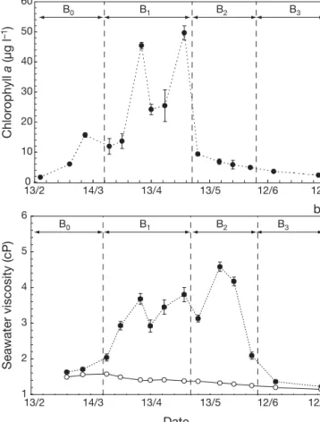
pennate Pseudonitzschia pseudodelicatissima (35 μm 1 2 3 4 5 6 0 10 20 30 40 50 60 B₀ 13/2 14/3 13/4 13/5 12/6 12/7 13/2 14/3 13/4 13/5 12/6 12/7 Seawater viscosity (cP) Date Chlor ophyll a (µg l –1 ) a b B₁ B₂ B₃ B₀ B₁ B₂ B₃

Fig. 1. Time course of (a) chl a concentration (μg l–1_{) and (b)} seawater viscosity (cP). B0is the pre-bloom period, B1and B2 are the Phaeocystis globosa bloom periods respectively

before and after the formation of foam, and B3 is the post-bloom period. In (B) note the difference between the (d₎ mea-sured seawater viscosity ηmand the (s) physically controlled

viscosity component ηT,Sestimated from viscosity

measure-ments conducted on filtered (0.20 μm mesh size) seawater from the same samples. Error bars represent ± SD

length, 0.1 × 104_{to 11.2× 10}4_{cells l}–1_{); (3) a post-bloom}

assemblage characterized by Guinardia delicatula

(30 μm length, 3.8× 105_{to 8.0× 10}5_{cells l}–1_), Leptocylin-drus spp. (L. danicus and L. minimus; 20 to 35 μm length,

0.7 × 105_{to 3.7 × 10}5_{cells l}–1_{) and the large fine-walled}

species of the genus Rhizosolenia spp. (R. setigera and R. imbricata; ≥300 μm length, 1.0 × 104

to 7.0 × 104_{cells l}–1_{). Two abundance maxima were observed,}

the first on April 8 with a concentration of 1.7 × 106_{cells l}–1_{when the phytoplankton assemblage was}

highly dominated by Phaeocystis globosa, and the

sec-ond on June 15 with a concentration of 2.8 × 106_{cells l}–1

when P. globosa had disappeared. The first peak was

mainly due to chain-forming species such as Chaeto-ceros sp., G. delicatula and P. pseudodelicatissima. In

particular, P. pseudodelicatissima and Chaetoceros sp.

were observed to be embedded into P. globosa colonies.

The second peak was strongly dominated by Chaetoceros sp. that reached 2.1× 106

cells l–1_.

Cryptophyceans (7 μm) were at times abundant before and after the Phaeo-cystis globosa bloom, reaching ca. 20%

and 10%, respectively, of total protist abundance (Table 2). The correspond-ing carbon biomass (0.1 to 0.6 μgC l–1₎

was always <1% of the total protist car-bon biomass.

Dinoflagellates were less abundant with maximum abundance values never exceeding 6.0 × 105_{cells l}–1_{, which}

cor-responded to a maximum relative abun-dance smaller than 15% (Table 2). Their carbon biomass were nevertheless bounded between 0.3 and 195.4 μgC l–1_,

and represented 30.0% and 28.4% of total protist carbon biomass before the

Phaeocystis globosa bloom (B0) and after the formation of foam (B2),

respec-tively. The dinoflagellate pool was dom-inated by small forms (25 μm in length) constituting > 70% of total dinoflagel-late abundance followed by large het-erotrophic Gyrodinium lachryma (160

μm length, 1 to 11%) and Protoperi-dinium sp. (50 μm length, 1 to 30%).

Finally, ciliated protozoans reached their maximum concentrations before the bloom (7.0 × 103_{cells l}–1_{) and during}

the Phaeocystis globosa bloom before

the formation of foam (1.0 × 104_{cells l}–1_),

representing < 0.5% of total protists. These abundances correspond to car-bon biomass ranging from 1.5 to 27.6 μgC l–1_{, representing 0.2 to 23.9% of}

total protist carbon biomass. Contributions of dinofla-gellates and ciliates to total protist carbon were not negligible particularly before (up to 54%, period B0)

and during the P. globosa bloom after the formation of

foam (0.6 to 30.1%, period B1).

Temporal patterns in Phaeocystis globosa spring

bloom

Four distinct periods were identified according to the previously mentioned chlorophyll concentration, sea-water excess viscosity and phytoplankton taxonomy and abundance, and defined according to the follow-ing criteria:

(1) A pre-bloom period characterized by the absence of Phaeocystis globosa cells, low chlorophyll concen-Table 2. Abundance (cells l–1_{), relative abundance (% of total protists), biomass}

(μgC l–1_{) and relative biomass (% of total protist biomass) of the main protist} groups (autotroph and hetero/mixotroph) or species identified over the course of our survey. B0is the pre-bloom period, B1and B2are the Phaeocystis globosa bloom periods respectively before and after the formation of foam, and B3is the

post-bloom period

Trophic status, Abundance Relative Biomass Relative group/species, (cells l–1_{) abundance (μgC l}–1_{) biomass}

and bloom period (%) (%)

Autotrophs P. globosa B0 0.0 0.0 0.0 0.0 B1 0.8 × 10– 6–5.5 × 10– 6 40.4–80.5 99.8–676.4 7.2–67.8 B2 0.0–3.5 × 10– 6 0.0–45.2 0.0–437.7 0.0–54.8 B3 0.0 0.0 0.0 0.0 Nanoflagellates B0 0.6 × 10– 6–1.3 × 10– 6 50.8–74.8 1.2–2.0 0.5–5.7 B1 0.1 × 10– 6–1.1 × 10– 6 3.3–30.8 0.1–1.9 0.0–0.4 B2 2.0 × 10– 6–9.0 × 10– 6 41.7–82.0 0.3–17.3 0.5–3.4 B3 1.0 × 10– 6–1.1 × 10– 6 26.9–43.2 1.9–2.0 0.1–0.4 Diatoms B0 1.6 × 10– 5–5.2 × 10– 5 11.5–31.1 14.8–408.1 40.8–94.9 B1 2.3 × 10– 5–17.4 × 10– 5 9.6–45.9 54.9–1877.3 18.3–90.3 B2 7.3 × 10– 5–13.4 × 10– 5 6.4–31.7 315.9–476.3 44.0–69.4 B3 11 × 10– 5–27.6 × 10– 5 43.4–71.9 331.3–1518.4 79.9–92.7 Cryptophyceans B0 1.5 × 10– 5–3.5 × 10– 5 10.1–17.6 1.2–2.3 0.1–1.4 B1 0.1 × 10– 5–0.7 × 10– 5 0.1–2.6 0.1–1.2 < 0.1 B2 0.4 × 10– 5–2.7 × 10– 5 0.5–6.4 0.1–0.4 < 0.1 B3 0.5 × 10– 5–2.7 × 10– 5 0.1–10.7 0.1–0.4 < 0.1 Hetero/mixotrophs Dinoflagellates B0 0.1 × 10– 4–4.7 × 10– 4 0.1–3.2 6.6–11.0 0.5–30.7 B1 0.8 × 10– 4–3.0 × 10– 4 0.2–1.5 9.3–31.1 0.5–10.4 B2 0.5 × 10– 4–60.0 × 10– 4 0.1–14.2 1.1–195.4 0.1–28.5 B3 3.6 × 10– 4–6.6 × 10– 4 0.9–2.6 78.9–111.6 6.8–19.0 Ciliates B0 5.0 × 10– 3–7.0 × 10– 3 0.3–0.5 6.6–12.3 2.8–22.1 B1 1.4 × 10– 3–10.0 × 10– 3 0.1–0.4 3.7–24.7 0.1–4.3 B2 1.4 × 10– 3–2.8 × 10– 3 0.0–0.1 1.3–10.3 0.2–1.5 B3 1.0 × 10– 3–2.6 × 10– 3 0.0–0.1 2.5–5.6 0.3–0.6

tration, low seawater excess viscosity and dominated by nanoflagellates;

(2) A bloom period characterized by the presence of

Phaeocystis globosa cells and colonies, before the

for-mation of foam in the turbulent surf zone, increasing chlorophyll concentration and excess seawater excess viscosity and dominated by P. globosa;

(3) A bloom period characterized by the presence of

Phaeocystis globosa cells and senescent colonies, after

the formation of foam in the turbulent surf zone, a sharp decrease in chlorophyll concentration, an addi-tional increase in excess viscosity towards a maximum value, the appearance of ciliates and dinoflagellates and dominated by P. globosa and nanoflagellates;

(4) A post-bloom period characterized by the disap-pearance of Phaeocystis globosa cells, low chlorophyll

concentration, low seawater excess viscosity, a de-crease in ciliates and an inde-crease in dinoflagellates although protist assemblages remained dominated by diatoms and nanoflagellates.

These 4 periods will be respectively be referred to as B0, B1, B2and B3hereafter.

Gut content and swimming behaviour

Gut content. The gut content (GC) of Temora

longi-cornis adult females ranged from 0.13 to 1.40 ng

chlorophyll individual [ind.]–1 _{and was significantly}

different among the 4 periods identified above (KW and J tests, p < 0.01, Table 3). The temporal pattern of GC (Fig. 2) can be directly related to those observed for chlorophyll concentration, seawater viscosity (Fig. 1) and protist taxonomy (Table 2). Gut content significantly increased (Kendall’s τ, p < 0.01) from 0.45 ± 0.02 to 0.55 ± 0.08 ng chlorophyll ind.–1₍x ± SD)

during the pre-bloom period B0, i.e. when diatoms

(Thalassiosira rotula, Skeletonema costatum and Aste-rionellopsis glacialis) constituted the bulk of carbon

biomass. Despite the sharp increase in chlorophyll due to Phaeocystis globosa bloom between March 29 and

April 30 (period B1; Fig. 1a), GC significantly

de-creased (p < 0.01) from 0.65 ± 0.04 ng chlorophyll ind.–1

(x ± SD) to 0.34 ± 0.05 ng chlorophyll ind.–1_{(Fig. 2) with}

increasing seawater viscosity (Fig. 1b). Thereafter, GC sharply increased with the formation of foam (period B2) to reach a maximum of 1.44 ± 0.13 ng chlorophyll

ind.–1_{on May 18, despite a 5-fold decrease in}

chloro-phyll concentration and the appearance of hetero-trophic protists. Gut content then decreased to 0.43 ± 0.10 ng chlorophyll ind.–1_{on June 6 (Fig. 2) and finally}

dropped down to 0.13 ± 0.01 ng chlorophyll ind.–1_after

the bloom when P. globosa is replaced by large fine

walled diatoms (Fig. 2, Tables 2 & 3).

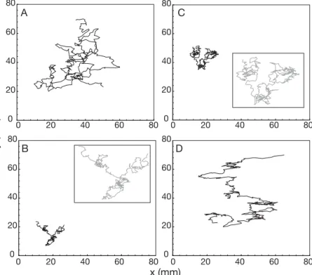
Swimming paths. Two types of convoluted

swim-ming paths were visually identified for Temora lon-gicornis adult females (Fig. 3). During the pre- and

post-bloom periods, swimming paths were relatively isotropic and characterized by their large spatial ex-tent, with distances of mostly 4 to 6 cm travelled in 20 to 30 s (Fig. 3a,d). In contrast, during the 2 bloom periods, swimming paths were more localized, with maximal horizontal and vertical extents always less than than 2 cm and characterized by an alternation Table 3. Temora longicornis. Ranges of chl a concentration (μg l–1_{), seawater viscosity (η}

m, cP) and the behavioural parameters

estimated for adult females; gut content (GC, ng chlorophyll ind.–1_{), swimming speed (}

v, mm s–1_{), net –gross displacement rate} (NGDR), swimming activity index (Ai, %) and fractal dimension D. B0is the pre-bloom period, B1and B2are the Phaeocystis

globosa bloom periods respectively before and after the formation of foam, and B3is the post-bloom period Bloom Chl a (μg l–1_{) η} m(cP) GC v (mm s–1) NGDR Ai D period (ng chl ind.–1₎ B0 0.78–15.70 1.62–1.71 0.45–0.55 1.12–1.20 0.63–0.67 97.4–96.9 1.18–1.20 B1 11.94–49.68 2.04–3.80 0.35–0.67 0.44–1.02 0.63–0.69 22.4–92.7 1.19–1.52 B2 4.89–9.37 2.09–4.59 0.43–1.44 0.38–0.95 0.65–0.68 42.8–79.0 1.53–1.82 B3 2.58–3.62 1.23–1.36 0.13–0.19 1.10–1.20 0.65–0.66 94.0–99.0 1.23–1.24 0.0 0.6 1.2 1.8 2.4 13/2 14/3 13/4 13/5 12/6 12/7

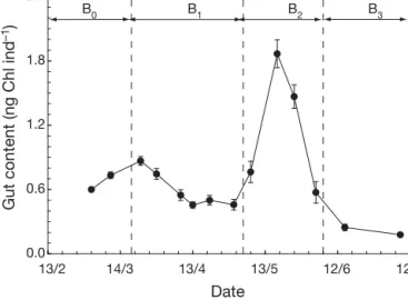
Gut content (ng Chl ind

–1

)

Date

B₀ B₁ B₂ B₃

Fig. 2. Temora longicornis. Time course of gut contents GC

(ng chlorophyll ind.–1_{) of adult females. B}

0is the pre-bloom period, B1and B2are the Phaeocystis globosa bloom periods respectively before and after the formation of foam, and B3is

between relatively linear and highly convoluted swimming paths (Fig. 3b,c). Swimming speed, swimming activity

index and NGDR. The swimming speed

of Temora longicornis adult females

ranged from 0.38 to 1.20 mm s–1_{(0.76 ±}

0.32 mm s–1_, x ± SD), and significantly

differed over the course of the survey (KW test, p < 0.01, Fig. 4a, Table 3). The swimming speed recorded during the pre- and post-bloom periods, B0(1.16 ±

0.06 mm s–1_{) and B}

3(1.15 ± 0.07 mm s–1),

were not distinguishable (J test, p > 0.05) and significantly higher (p < 0.01) than those observed during the bloom periods B1(0.63 ± 0.23 mm s–1) and B2(0.56 ±

0.26 mm s–1_).

The swimming activity index Ai

(Fig. 4b) is bounded between 22.4 and 99.0 (63.1 ± 30.5, x ± SD). Swimming activity Ai was maximum during the

pre- and post-bloom periods B0(97.2 ±

0.4) and B3(96.5 ± 3.5), decreased

dur-ing the period B1from 92.7 to 22.4 and

increased from 42.8 to 79.0 during the period B2 (Fig. 4b). In contrast, the 0 20 40 60 80 0 20 40 60 80 0 20 40 60 80 0 20 40 60 80 0 20 40 60 80 0 20 40 60 80 0 20 40 60 80 0 20 40 60 80 x (mm) y (mm) A C B D

Fig. 3. Temora longicornis. Swimming trajectories of adult females recorded

(A) before (period B0) and (D) after (period B3) the Phaeocystis globosa bloom, and during the bloom (B) before (period B1) and (C) after (period B2) the

forma-tion of foam. The inserts are magnificaforma-tions of the actual trajectories

0.0 0.2 0.4 0.6 0.8 1.0 1.2 1.4 13.2 14.3 13.4 13.5 12.6 12.7 0 20 40 60 80 100 13.2 14.3 13.4 13.5 12.6 12.7 0.5 0.6 0.7 0.8 13.2 14.3 13.4 13.5 12.6 12.7 1.0 1.2 1.4 1.6 1.8 2.0 13.2 14.3 13.4 13.5 12.6 12.7 Swimming speed (mm s –1) Activity index Ai Fractal dimension NGDR Date A C B D B₀ B₁ B₂ B₃ B₀ B₁ B₂ B₃ B₀ B₁ B₂ B₃ B₀ B₁ B₂ B₃

Fig. 4. Temora longicornis. Time course of the behavioural parameters of adult females; (A) swimming speed (mm s–1_{), (B)} activ-ity index (%), (C) NGDR and (D) fractal dimension D. B0is the pre-bloom period, B1and B2are the Phaeocystis globosa bloom

NGDR of T. longicornis adult females ranged from 0.63

to 0.69 (0.66 ± 0.01, x ± SD) and did not exhibit any sig-nificant difference over the course of the survey (KW test, p > 0.05, Fig. 4c).

Fractal dimension. Plots of logLδ versus logδ (Eq. 8)

and N (λ) versus λ (Eq. 10) exhibited very strong linear

behaviours over the whole range of available scales (not shown) with coefficients of determination (r2₎

ranging from 0.98 to 0.99, and always satisfied the 2 optimisation criteria described above. The compass fractal dimension Dc and the box-counting fractal

dimension Dbwere not significantly different (U-test,

p > 0.05). As a consequence, the results obtained for fractal dimension estimates Dcand Dbwill be referred

to as the fractal dimension D, where:

(11)

Ncand Nbare the numbers of compass dimension Dc

and box-counting dimension Db estimates,

respec-tively (Nc= Nb= 5).

The fractal dimension D estimated for the swimming

paths observed over the course of the survey were sig-nificantly different (KW test, p < 0.01, Fig. 4d) and exhibited significant differences between each of the 4 periods B0, B1, B2and B3(J test, p < 0.01, Table 3). The

highest and lowest fractal dimensions were found for the pre-bloom period B0(D = 1.19 ± 0.01) and during

the bloom period B2after the formation of foam (D =

1.68 ± 0.12). Intermediate values were found for the periods B3(D = 1.24 ± 0.01) and B1(D = 1.38 ± 0.12).

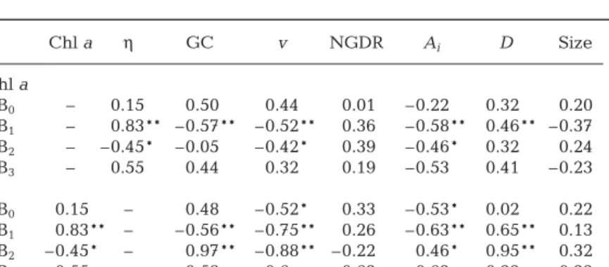
Correlation analyses. The potential relationship

be-tween chlorophyll concentration, seawater viscosity and the parameters related to the feeding and swim-ming behaviour of Temora longicornis adult females

were investigated through correlation analysis for

each of the 4 periods B0, B1, B2and B3described

pre-viously (Table 4). Chlorophyll concentration and sea-water viscosity were significantly correlated both positively and negatively during the bloom period res-pectively before and after the formation of foam. No significant correlations were found between chloro-phyll concentration and T. longicornis feeding and

swimming behaviour during the pre- and post-bloom periods B0and B3. In contrast, before the formation of

foam, chlorophyll concentration was negatively corre-lated (p < 0.01) with gut content, swimming speed and swimming activity and positively correlated with frac-tal dimension. After the formation of foam, chlorophyll concentration was negatively correlated (p < 0.01) with swimming speed and swimming activity (Table 4). During the pre-bloom period B0, swimming speed and

swimming activity were negatively correlated (p < 0.05) with seawater viscosity. During the bloom, gut content and swimming activity were negatively and positively correlated (p < 0.01) with viscosity before and after the formation of foam, respectively. In con-trast, swimming speed and fractal dimension respec-tively were always negarespec-tively and posirespec-tively corre-lated (p < 0.01) to viscosity. No significant correlations were found between the feeding and swimming behaviour of T. longicornis and seawater viscosity

dur-ing the post-bloom period B3.

DISCUSSION

Chlorophyll concentration, seawater viscosity and foam formation

The shift from positive to negative significant corre-lations between chlorophyll concentration and sea-water viscosity before and after the foam formation (Table 4) is congruent with a recent mechanistic explanation (Seuront et al. 2006) suggesting that the disruption of the mucilaginous colo-nial matrix by turbulent mixing leads to (1) the formation of foam and the re-lease of flagellated cells, (2) a decrease in chl a concentration (Fig. 1a) as a

sig-nificant proportion of cells are entrained within the foam during the emulsion process, and finally (3) the decoupling between the viscous (i.e. colonial polymeric materials) and non-viscous (flagellated cells) contribution of Phaeocystis globosa to bulk phase

seawater properties. This is also consis-tent with the dynamics of transparent exopolymeric particles (TEP) produced

D N_c Dc N D N b b N c b = 1

∑

∑

Table 4. Temora longicornis. Spearman rank correlations (ρ) between chl a

con-centration, seawater viscosity (η), and the related behavioural parameters esti-mated for adult females: gut content (GC), swimming speed (v), net –gross

dis-placement rate (NGDR), swimming activity index (Ai), fractal dimension (D ) and

the size of adult females. B0is the pre-bloom period, B1and B2are the

Phaeocys-tis globosa bloom periods respectively before and after the formation of foam,

and B3is the post-bloom period. *5% significance level, **1% significance level

Chl a η GC v NGDR Ai D Size Chl a B0 – 0.15 0.50 0.44 0.01 –0.22 0.32 0.20 B1 – 0.83** –0.57** –0.52** 0.36 –0.58** 0.46** –0.37 B2 – –0.45* –0.05 –0.42* 0.39 –0.46* 0.32 0.24 B3 – 0.55 0.44 0.32 0.19 –0.53 0.41 –0.23 η B0 0.15 – 0.48 –0.52* 0.33 –0.53* 0.02 0.22 B1 0.83** – –0.56** –0.75** 0.26 –0.63** 0.65** 0.13 B2 –0.45* – 0.97** –0.88** –0.22 0.46* 0.95** 0.32 B3 0.55 – 0.58 0.6 0.62 –0.62 0.22 0.22

by P. globosa (Mari et al. 2005). During the growth

phase of P. globosa, TEP and chl a concentration were

positively correlated. In contrast, the release of large TEP from the mucilaginous matrix of P. globosa

colonies after colony disruption leads to a negative cor-relation between TEP and chl a concentration. The

variety of dissolved particulate carbohydrates pro-duced during a P. globosa bloom (see van Rijssel et al.

2000 for a review) are known to coagulate sponta-neously via colloidal precursors and to form gel-like material in the shape of spheres, strings or sheets (Passow 2000). They are then likely to contribute to the formation of microscopic polymer gels in seawater (Chin et al. 1998) and, in turn, to affect seawater viscosity and the related microscale processes such as nutrient uptake, viral infection, feeding and swimming behaviour.

Chlorophyll concentration, seawater viscosity and zooplankton gut content

On the size mismatch and mechanical hindrance

hypothesis. While the research devoted to relate

sea-water viscosity measurement to the quality and the quantity of dissolved and particulate carbohydrates and transparent exopolymeric particles is still to be done, the exudates and transparent exopolymeric par-ticles derived from a Phaeocystis globosa dominated

community have been shown to inhibit copepod feed-ing on co-occurrfeed-ing phytoplankton preys (Dutz et al. 2005). This is consistent with the negative correlations observed between the gut content of Temora longicor-nis adult females (Fig. 2) and both chlorophyll

concen-tration and seawater viscosity during the first phase of the bloom (period B1; Fig. 1, Table 4). Despite a 4-fold

increase in chlorophyll concentration (Fig. 1a), gut contents significantly decreased (Fig. 2). This is con-gruent with the decrease in diatom ingestion (up to 25%) observed during blooms of P. globosa (Gasparini

et al. 2000, Koski et al. 2005), and suggests a defence strategy against zooplankton grazers through (1) the mechanical hindrance related to the increase in sea-water viscosity and/or (2) the size mismatch related to the embedding of P. globosa cells and non-motile

preys (mainly diatoms) in the colonial matrix (Koski et al. 2005). As a consequence, while P. globosa, Chaeto-ceros sp., Rhizosolenia imbricata, Guinardia delicatula,

and Pseudonitzschia pseudodelicatissima accounted

for more than 80% of the total protist abundance dur-ing the period B1, the increase in chlorophyll

concen-tration did not imply any increase in food availability (Fig. 5b).

In contrast, after the formation of foam (period B2), Temora longicornis gut contents increased (Fig. 2)

des-pite a decrease in chlorophyll concentration (Fig. 1a) and a further increase in seawater viscosity (Fig. 1b). The foam formation, and the related colony disruption, leads to the release of flagellated colony cells in the bulk phase seawater (e.g. Peperzak et al. 2000), together with the diatoms still embedded in the dis-rupted colonial matrix (Seuront et al. 2006). This potentially results in an increase in food availability (Fig. 5c) despite the overall decrease in chlorophyll concentration (see Fig. 1a). This is also consistent with the reported zooplankton grazing on Phaeocystis sp.

solitary cells at high concentration (Cotonnec et al. 2001) and demonstrates that even elevated viscosity (i.e. up to 4.6 cP; Fig. 1b) does not inhibit zooplankton grazing on phytoplankton cells due to mechanical hin-drance as previously suggested (Weisse et al. 1994).

From size mismatch and mechanical hindrance to

prey switching behaviour. The high and relatively

sta-ble egg production and hatching success observed throughout the survey (Flamme 2004) show that Temo-ra longicornis were able to sustain their production

rates despite a drastic change in the taxonomy of the protist resource. Given the negative correlation be-tween gut content and chlorophyll concentration, this suggests that the gut contents observed during the periods B1and B2(Fig. 2, Table 3) may be triggered by

the temporal dynamic of the protist community and the related prey switching behaviour.

Three non-conflicting hypotheses can then be sug-gested to explain the decrease in gut content observed during the period B1:

(1) A sharp decrease occurs in cryptophyceans (from 14.7 ± 3.2 to 1.5 ± 0.9% of total protists) that are actively selected by Temora longicornis in the eastern

English Channel (Cotonnec et al. 2001) during period B1, together with the dominance of toxin producers

(Pseudonitzschia pseudodelicatissima; e.g. Adams et

al. 2006). Although this potential prey avoidance still needs to be confirmed, it is consistent with the prey switching behaviour from phytoplankton to microzoo-plankton previously suggested for T. longicornis

dur-ing Phaeocystis globosa blooms (e.g. Gasparini et al.

2000; Fig. 5b).

(2) Heterotrophic ciliates are reported to be actively grazed by copepods; see Sanders & Wickham (1993) for a review. Their ingestion by copepods may then weaken the gut content signal (chl a) when compared

with a true phytoplankton-based diet. The high nutri-tive value of ciliates (Gifford 1991) allows for a better growth and survival of copepods (Sanders & Wickham 1993), and is consistent with the lack of decrease in production rate and hatching success despite the decrease in gut content.

(3) Ciliates also exert high grazing pressure on phytoplankton (>100% d–1_{; Sautour et al. 2000), and}

hence, may compete for food resource with copepods. This trophic competi-tion is consistent with the observed decrease in copepod gut contents coin-ciding with the peak of ciliate abun-dance (Acineta sp. and tintinnids).

In contrast, the high gut contents ob-served during period B2 (Fig. 5c) may

originate from active feeding on sheets of the disrupted colonial matrix and em-bedded phytoplankton cells (Koski et al. 2005), the sharp increase in abundance and biomass of dinoflagellates (Table 2) that typically represent a significant fraction of Temora longicornis diet (20 to

40%; Koski et al. 2005), and the shift from potentially toxic small sized di-atoms (e.g. Pseudonitzschia pseudo-delicatissima) to more palatable large

cells (e.g. Guinardia striata, Leptocylin-drus danicus).

Finally, at the end of the survey (period B3; Fig. 5d) low gut content

values may originate from both the de-crease in heterotrophic protist abun-dance and the disappearance of Phaeo-cystis globosa senescent colonies, thus

confirming the hypothesis of significant grazing on both these prey types after foam formation (period B2).

Chlorophyll concentration, seawater viscosity and swimming behaviour The behavioural properties of Temo-ra longicornis adult females suggest a

shift in their foraging activity related to the temporal dynamics of the Phaeocys-tis globosa bloom. While the significant

decrease observed in their swimming speed during the bloom (i.e. periods B1

and B2; Fig. 4a & Table 3) might be an

adaptive strategy to an increase in vis-cosity, this is very unlikely as the energy cost of swimming for T. longi-cornis represents only a negligible

frac-tion of the total energy consumpfrac-tion (see Table 5 in van Duren et al. 2006). Changes in copepod swimming behav-iour could, however, also be a response to the spatial distribution of prey organ-isms. According to the optimal foraging theory (Pyke 1984), organisms living in highly heterogeneous environments Fig. 5. Temora longicornis. Schematic illustration of feeding and swimming

be-haviour of adult females over the course of a Phaeocystis globosa spring bloom.

(A) Before and (D) after the P. globosa bloom, gut contents are directly controlled

by chl a concentrations and T. longicornis do not exhibit any specific foraging

be-haviour. In contrast (B & C), during the bloom T. longicornis exhibit elevated

aging activity despite low and high gut contents (B) before and (C) after the for-mation of foam, respectively. Before the forfor-mation of foam (B), phytoplankton cells are unavailable (or decreased drastically, e.g. cryptophyceans) or unsuitable to T. longicornis as they are embedded in the mucilaginous colonial materials

(e.g. diatoms) or potentially toxic species (e.g. Pseudonitzschia pseudodelicatis-sima). After the formation of foam (C), despite a lower chl a concentration, P. glo-bosa cells released from mucilaginous materials along with colonial fragments

containing embedded phytoplankton cells become available to grazers. As egg production did not exhibit any significant differences over the duration of the sur-vey, it is also suggested that T. longicornis have the ability to switch their feeding

behaviour from phytoplankton to microzooplankton (A–B) and from microzoo-plankton to phytomicrozoo-plankton (B–C), depending on the availability of P. globosa

cells. ( ) P. globosa cells, ( , ,, , ) phytoplankton cells other than P. globosa

could develop strategies to exploit high density patches and then optimise the energy required to cap-ture a given amount of food. This can be achieved by increasing the complexity of swimming paths with increasing food density and/or decreasing the swim-ming speed or the motility in food patches, thus result-ing in an area-restricted searchresult-ing strategy (e.g. Jons-son & JohansJons-son 1997). The time course of fractal dimension D (Fig. 4d) indicates an increased foraging

activity during the P. globosa bloom (i.e. periods B1and B2) that might be related to more patchy food

distribu-tions. This is consistent with recent observations show-ing an increase in chl a patchiness during the P. glo-bosa bloom in the coastal waters of the eastern English

Channel for scales relevant to copepods, i.e. 5 to 50 cm (Seuront et al. 2007). Healthy and senescent P. globosa

colonies and their embedded cells are also likely to contribute to this patchiness. Before and after the

P. globosa bloom, chl a is more homogeneously

distrib-uted (Seuront et al. 2007), resulting in more rectilinear swimming paths (Figs. 3a,b & 5a,d). The gut contents are then directly controlled by the amount of chl a in

the environment. In contrast, during the bloom chl a is

more heterogeneously distributed (Fig. 5b,c) and the microscale hotspots of organic matter related to colony formation and/or disruption are also likely to represent a secondary source of patchiness for bacteria and microzooplankton grazers. This results in more convo-luted swimming paths related to an area-restricted searching strategy of copepods preying on microzoo-plankton organisms before the formation of foam (period B1; Fig. 5b). This is supported by the

sustain-ability of T. longicornis egg production (Flamme 2004)

despite low gut contents (Fig. 2) and is consistent with the previously mentioned relative unavailability and/or unsuitability of the phytoplankton resource, a potential trophic competition with large ciliates and the subsequent decrease in chl a gut content (Fig. 5b).

After the foam formation, convoluted swimming paths might also be related to an area-restricted searching strategy of copepods preying on phytoplankton cells released in the bulk phase seawater from the mucilagi-nous materials after the formation of foam, on senes-cent colonies and/or on large fine walled diatoms still embedded in colonial materials (Fig. 5c). The steady behaviour of the NGDR over the course of the bloom confirms previous studies stating that it is a far less accurate and ecologically relevant index of curviness than the fractal dimension; see Seuront et al. (2004) for a discussion.

While this issue is beyond the scope of the present work, it is finally suggested that the individual-scale behavioural processes observed in response to fluctua-tions in the biophysical properties of the local environ-ment ultimately are likely to cascade from the scale of

the individual grazers up to larger scale and to influ-ence critical processes such as biogeochemical fluxes through their control of zooplankton trophodynamics and production rates. This is especially relevant in the framework of Phaeocystis sp. blooms, given the

near-global distribution and the key role played by the genus Phaeocystis in the ocean–atmosphere transfers.

Acknowledgements. We acknowledge the captain and the

crew of the NO ‘Sepia II’ for their help during the sampling experiment, and 2 anonymous reviewers whose comments and criticisms greatly improved a previous version of this work. E. Lecuyer and G. Flamme are acknowledged for their contribution to the field work. This work was supported by the CPER ‘Phaeocystis’, PNEC ‘Chantier Manche Orientale-Sud Mer du Nord’, Centre National de la Recherche Scien-tifique, Université des Sciences et Technologies de Lille, Aus-tralian Research Council and Flinders University.

LITERATURE CITED

Adams NG, MacFadyen A, Hickey BM, Trainer VL (2006) The nearshore advection of a toxigenic Pseudo-nitzschia

bloom and subsequent domoic acid contamination of intertidal bivalves. Afr J Mar Sci 28:271–276

Bratbak G, Jacobsen A, Heldal M (1998) Viral lysis of Phaeo-cystis pouchetii and bacterial secondary production.

Aquat Microb Ecol 16:11–16

Chen YQ, Wang N, Zhang P, Zhou H, Qu LH (2002) Molecu-lar evidence identifies bloom-forming Phaeocystis

(Pry-mensiophyta) from coastal waters of southeast China as

Phaeocystis globosa. Biochem Syst Ecol 30:15–22

Chin WC, Orellana MV, Verdugo P (1998) Spontaneous assembly of marine dissolved organic matter into polymer gels. Nature 391:568–572

Cotonnec G, Brunet C, Sautour B, Thoumelin G (2001) Nutri-tive value and selection of food particles by copepods during a spring bloom of Phaeocystis sp. in the English

Channel, as determined by pigment and fatty acid analy-ses. J Plankton Res 23:693–703

Dagg MJ, Wyman KD (1983) Natural ingestion rates of the copepods Neocalanus plumchrus and N. cristatus

calcu-lated from gut contents. Mar Ecol Prog Ser 13:37–46 Dam HG, Peterson WT (1993) Seasonal contrasts in the diel

vertical distribution, feeding behavior and grazing impact of the copepod Temora longicornis in Long Island Sound.

J Mar Res 51:561–594

Dutz J, Klein Breteler WCM, Kramer G (2005) Inhibition of copepod feeding by exudates and transparent exopolymer particles (TEP) derived from a Phaeocystis globosa

do-minated phytoplankton community. Harmful Algae 4: 929–940

Flamme G (2004) Effets de la nourriture et de la temperature sur les triats du cycle de vie du copépode Temora longicornis

(Müller): couplage entre un suivi in situ et expérimental.

MSc thesis, Université des Sciences et Technologies de Lille Fransz HG, Gonzalez SR, Cadée GC, Hansen FC (1992) Long-term change of Temora longicornis (Copepoda,

Cala-noida) abundance in a Dutch tidal inlet (Marsdiep) in rela-tion to eutrophicarela-tion. Neth J Sea Res 30:23–32

Gasparini S, Daro MH, Antajan E, Tackx M, Rousseau V, Par-ent JY, Lancelot C (2000) Mesozooplankton grazing dur-ing the Phaeocystis globosa bloom in the southern bight of

the North Sea. J Sea Res 43:345–356

➤

➤

➤

➤

➤

➤

➤

➤