Shape and erosion of pebbles

HAL Id: hal-00144239

https://hal.archives-ouvertes.fr/hal-00144239

Submitted on 16 Jun 2007

HAL is a multi-disciplinary open access

archive for the deposit and dissemination of

sci-entific research documents, whether they are

pub-lished or not. The documents may come from

teaching and research institutions in France or

abroad, or from public or private research centers.

L’archive ouverte pluridisciplinaire HAL, est

destinée au dépôt et à la diffusion de documents

scientifiques de niveau recherche, publiés ou non,

émanant des établissements d’enseignement et de

recherche français ou étrangers, des laboratoires

publics ou privés.

Douglas Durian, H. Bideaud, P. Duringer, André Schröder, Carlos Marques

To cite this version:

Douglas Durian, H. Bideaud, P. Duringer, André Schröder, Carlos Marques. Shape and erosion of

pebbles. Physical Review E : Statistical, Nonlinear, and Soft Matter Physics, American Physical

Society, 2007, 75 (2), pp.021301. �10.1103/PhysRevE.75.021301�. �hal-00144239�

The shape and erosion of pebbles

Department of Physics & Astronomy, University of Pennsylvania, Philadelphia, PA 19104-6396, USA

2

LDFC-CNRS UMR 7506, 3 rue de l’Universit´e, 67084 Strasbourg Cedex, France and

3

CGS-CNRS UMR 7517, Institut de G´eologie, 1 rue Blessig, 67084 Strasbourg Cedex, France (Dated: November 28, 2006)

The shapes of flat pebbles may be characterized in terms of the statistical distribution of curvatures measured along their contours. We illustrate this new method for clay pebbles eroded in a controlled laboratory apparatus, and also for naturally-occurring rip-up clasts formed and eroded in the Mont St.-Michel bay. We find that the curvature distribution allows finer discrimination than traditional measures of aspect ratios. Furthermore, it connects to the microscopic action of erosion processes that are typically faster at protruding regions of high curvature. We discuss in detail how the curvature may be reliable deduced from digital photographs.

PACS numbers: 45.70.-n,83.80.Nb,91.60.-x,02.60.Jh

I. INTRODUCTION

The roundness of pebbles on a beach has long been a source of wonder and astonishment for scientists in many fields [1, 2]. Explanations for the pebble shapes were born from the simple pleasure of understanding nature but also from the hope that a pebble, or a collection of pebbles, might carry lithographically imprinted the signature of their erosion history. Reading that imprint would then, for instance, reveal if a pebble was eroded on a beach, a river or a glacier, or if it traveled a long distance down a stream. It even perhaps would reveal for how long the erosion forces have been at work on that object. Of obvious interest in Geology [3], a physical understand-ing of the formation of erosion shapes would also allow for a better control of many industrial processes lead-ing to rounded objects such as gem stone or clay bead grinding in tumblers or fruit and vegetable peeling in sev-eral mechanical devices. Diverse mathematical tools have been developed for geometrical shape analysis of crys-talites, cell membranes, and other far from equilibrium systems [4–7]; however, these do not seem applicable to pebbles.

The evolution of a pebble shape under erosion can ar-guably be viewed as a succession of elementary cuts that act at the surface of the body to remove a given amount of material. This converts young, polyhedral-like shapes with a relatively small number of large sides and sharp vertices into more mature shapes with a high number of small sides and smooth vertices. The size and the shapes of each of these successive ablations, as well as the surface sites where the cutting happens, are determined both by the conditions under which erosion takes place and by the nature of the material being eroded. Exposure of a young, polyhedral-like shape to the rough tumbling of a steep stream slope will result in relatively large cuts of the angular sections, while exposure to the gentle erosion of wind or water is more likely to lead to small cuts al-most parallel to the existing flat sides. Also, the same sequence of external forces acting on two identical origi-nal shapes of different materials will result into distinct

forms due to weight, hardness or anisotropy differences. In spite of the diversity of factors at play in shape mod-ification, the complete evolution of the pebble shape is fully determined by (i) the initial form described by some number of faces, edges and vertices and (ii) the position, size and orientation of the successive ablations.

Given that the erosion process evolves by a succession of localized events on the pebble surface, it is surprising that the majority of the precedent attempts to charac-terize the pebble shapes were restricted to the determi-nation of global quantities such as the pebble mass or the lengths of its three main axes [3]. Clearly, in order to capture both the local nature of the erosion process and the statistical character of the successive elementary cuts, one needs to build a new detailed description of the pebble shapes based on quantities that are more micro-scopic and more closely connected to evolution processes. In Ref. [8] we proposed curvature as a key microscopic variable, since, intuitively, protruding regions with large curvature erode faster than flatter regions of small cur-vature. We then proposed the distribution of curvature around a flat, two-dimensional, pebble as a new statisti-cal tool for shape description. And finally we illustrated and tested these ideas by measuring and modeling the erosion of clay pebbles in a controlled laboratory appa-ratus.

In this paper we elaborate on our initial Letter [8], and we apply our methods to naturally-occurring rip-up clasts found in the tidal flats of the Mont St.-Michel bay. Section II begins with a survey of shape quantifi-cation for two-dimensional objects, in general, and reca-pitulates our new curvature-based method. Section III provides further details of the laboratory experiments on clay pebbles. Section IV presents a new field study of the Mont St.-Michel rip-up clasts. And finally, following the conclusion, two methods are presented in the Appen-dix for reliably extracting the local curvature from digital photographs.

II. 2D SHAPE QUANTIFICATION

The issue of rock shape is of long-standing interest in the field of sedimentology [9–17]. Two basic methods have become sufficiently well established as to be dis-cussed in introductory textbooks [3]. The simplest is a visual chart for comparing a given rock against a stan-dard sequence of rocks that vary in their sphericity and angularity. A rock has high “sphericity” if its three di-mensions are nearly equal. And it is “very angular”, inde-pendent of its sphericity, if the surface has cusps or sharp ridges; the opposite of “very angular” is “well rounded”. While useful for exposition, such verbal distinctions are subjective and irreproducible. The second method is to form dimensionless shape indices based on the lengths of three orthogonal axes. From the ratios, and the ratios of differences, of the long to intermediate to short axes, one can readily distinguish rods from discs from spheres. And a given rock may be represented by a point on a triangular diagram according to the values of three such indices, with rod / disc / sphere attained at the corners. This practice is nearly half a century old [18]. Neverthe-less, there is still much debate about which of the infinite number of possible shape indices are most useful [19–23]. In any case, such indices cannot capture fine distinctions in shape, let alone the verbal distinctions of angular vs rounded. Furthermore, they provide no natural connec-tion to the underlying physical process by which the rock was formed.

More recent methods of shape analysis employ Fourier [24–28], or even wavelet [29], transforms of the contour. This applies naturally to flat pebbles or grains, but also to flat images of three-dimensional objects. The advantage of Fourier analysis over shape indices is that, with enough terms in the series, the exact pebble con-tour can be reproduced. For simple shapes, the concon-tour may be described in polar coordinates by radius (eg dis-tance from center of mass) vs angle, r(θ), and the corre-sponding transform. However, this representation is not single-valued for complex shapes with pits or overhangs. Generally, the contour may be described by Cartesian co-ordinates vs arclength, {x(s), y(s)}, and the correspond-ing transforms. In any case, the relative amplitudes of different harmonics give an indication of shape in terms of roughness at different length scales. In a different area of science, Fourier representations have proven es-pecially useful for analysis of fluctuations and instabili-ties of liquid interfaces, membranes, etc. [4–6]. In prac-tice, for these systems, shape fluctuations are sampled during some time interval and then the average Fourier amplitudes extracted by averaging over many different realizations of the shape. Also, because these phenom-ena are linear, each Fourier component grows or shrinks at some amplitude-independent rate and the evolution is fully determined by a dispersion relation. Unfortunately these features do not hold for the erosion of pebbles. Be-cause each pebble shape only provides one configuration, average quantities need to be built from a different

pre-scription. Also, there is no a priori guaranty that the variables are Gaussian distributed, and one needs a di-rect space method to better assess the importance of non-linear phenomena. Non-non-linearity is, we suspect, intrinsi-cally embedded in the erosion mechanisms of pebbles. If one considers for instance a shape represented by a single harmonic in the r(θ) representation, it is clear that the peaks will wear more rapidly than the valleys. Therefore the erosion rate cannot be a function of the harmonic number only; it must either be a non-linear function of the amplitude itself or a function coupling many harmon-ics.

Our aim is to provide an alternative measure of pebble shape that is well-defined, simple, and connects naturally to local properties involved in the evolution process. We restrict our attention to flat pebbles, where an obvious shape index is the aspect ratio of long to short axes. Since erosion processes generally act most strongly on the rough, pointed portions of a rock, we will focus on the local curvature of the pebble contour. Technically, curvature is a vector given by K = dT/ds, the deriva-tive of the unit tangent vector with respect to arclength along the contour [30]. More intuitively, the magnitude of the curvature is the reciprocal of the radius of a circle that mimics the local behavior of the contour. Here we shall adopt the sign convention K > 0 where the contour is convex (as at the tip of a bump) and K < 0 where the contour is concave (as where a chip or bite has been removed from an otherwise round pebble). In the Ap-pendix, we describe two means by which the curvature may be reliably measured at each point along the peb-ble contour. Note that the average curvature is simply related to the perimeter of the contour:

P = 2π/hKi, (1) which is obviously correct when the shape is a circle.

To describe the shape of a pebble, a very natural quan-tity is the distribution of curvatures, ρ(K), defined such that ρ(K)dK is the probability that the curvature at some point along the contour lies between K and K +dK [8]. In order to distinguish different distributions, as a practical matter, it is more reliable [31] to use the cumu-lative distribution of curvatures

f (K) = Z K

0

ρ(K′_)dK′ ₍₂₎

Literally, f (K) is the fraction of the perimeter with cur-vature less than K. Note that f (K) increases from 0 to 1 as K : 0 → ∞; the minimum curvature is where f (K) first rises above 0, the maximum curvature is where f (K) first reaches 1, and the median curvature is where f (K) = 1/2. Unlike for ρ(K), it is not necessary to bin the curvature data in order to deduce f (K). Instead, just sort the curvature data from smallest to largest and keep a running sum of the arclength segments, normalized by perimeter. Finally, so that the shapes of pebbles of dif-ferent sizes may be compared, it is useful to remove the

3 0 0.2 0.4 0.6 0.8 1 0 0.5 1 1.5 2 2.5 3 f(K) K/<K> (c) 0 1 2 3 0 π 0 . 5 π 1 π 1 . 5 π 2 π superellipse oval ellipse circle K/<K> θ (b) 0.9 1 1.1 1.2 1.3 1.4 1.5 1.6 r (a)

FIG. 1: (Color online) (a) Radius, (b) normalized curvature and (c) fraction of the perimeter f (K) with curvature less than K, vs K divided by the average curvature hKi, for a superellipse, oval, ellipse, and circle. The curve types match those for the shapes as shown in the inset. Note that, except for the circle, all have the same aspect ratio a = 3/2. The differences in shape are reflected in differences in the forms of f (K).

scale factor hKi, which is related to the total perimeter as noted above in Eq. (1). Altogether, we thus propose to quantify pebble shape by examining f (K) as a function of K/hKi.

To help build intuition, examples of f (K) are given in Fig. 1 for a few simple shapes. The simplest of all is a circle, where the curvature is the same at each point along the contour: K = hKi = 2π/P = 1/R. Thus f (K) = 0(1) for K < (>)hKi. The curvature distribu-tion is the derivative of this step funcdistribu-tion, giving ρ(K) = δ(K − hKi) as required. The other three shapes shown in Fig. 1 are all tangent at four points to the rectangular region {|x| < a = 3/2, |y| < 1}: an ellipse (x/a)2

+ y2

=1; a superellipse (x/a)4

+ y4

= 1; and an oval [x/a + (1 − 1/a)y2

/2]2

+ y2

= 1. For a general ellipse, with long and short axes a and b respectively, one may compute f (K) = E(sin−1_[1/ǫ(1−(2√_{1 − ǫ}2 E(ǫ2 )/(πK))2_/3 )1_/2 ], ǫ2 )/E(ǫ2 ) where ǫ =p1 − b2_/a2 _{is the ellipticity, E(x) is the}

com-plete elliptical integral of the first kind and E(x, m) is the incomplete elliptic integral of the second kind [30].

While the ellipse, superellipse, and oval in Fig. 1 all

have the same aspect ratio, a = 3/2, their shapes are obviously different. This emphasizes how a single num-ber is insufficient to quantify shape. The shape differ-ences do, however, show up nicely in the forms of f (K). The ellipse is closest to a circle, with a distribution of curvatures that is most narrowly distributed around the average and hence with an f (K) that is most like a step function. The superellipse is farthest from a circle, with four long nearly-flat sections and four high-curvature cor-ners; its curvature distribution is broadest. The oval is intermediate.

III. LABORATORY EXPERIMENT

The examples given in Fig. 1 correspond to regular, highly symmetric shapes of two dimensional convex “peb-bles”. In practice, natural or artificial erosion processes lead to curvature functions with an important statistical component. In this section we elaborate on the labora-tory experiments of Ref. [8], designed to study both the statistical nature of the curvature distribution and the in-fluence of the original shapes of the pebbles on the final output of a controlled erosion process.

Laboratory pebbles were formed from “chamotte” clay, a kind of clay made from Kaolin and purchased from Graphigro, France. The water content of the purchased clay was 22% in a state that could easily be kneaded. The clay was kept tightly packed before use in order to avoid water evaporation. Clay pebbles were produced using aluminium molds made in our laboratory. They consist of a polygonal well of 0.5 cm depth. Once the mould was filled with clay, it was left at rest for 24 hours, so that 98.5% of the water was removed by evaporation. All the experimental results presented here concern one day old pebbles. We noticed that pebbles older than 2 days were too fragile for our experimental configuration. The number of samples and the dimensions of the various pebbles are as follows: four squares of side 5 cm, five rectangles of sides 4 × 6 cm2

, five regular pentagons of side 4.25 cm, one triangle with sides {7 cm, 7.5 cm, 9 cm}, one irregular polygon with 7 sides, one lozenge with acute angles of 45◦ _{and four sides of 5 cm, and one circle of}

diameter 7 cm.

The wearing method that we chose relies on placing a pebble in the rotating apparatus sketched in Fig. 2. The apparatus is a square basin, of dimensions 30×30×7 cm3

. The basin bottom is a 1 cm thick aluminium plate and the walls are made of 0.04 cm thick aluminium sheets. This rotating plate is fixed to a rod held by the jaws of a laboratory mixer, Heidolph RZR1. The mixer itself is fixed to a tripod, so that its inclination angle can be varied.

A typical trajectory of the pebble during the continu-ous rotation of the plate can be described as follows. First the pebble rotates with the basin until it reaches a high position. After the plate has rotated an angle between π/2 and π, the pebble begins to slide due to gravity, until

FIG. 2: The wearing apparatus used for the laboratory ex-periments. The rotating metal tray is 30 × 30 × 7 cm3

.

it hits one of the walls in the bottom part of the container, and then rolls down along that wall as the basin keeps its rotation. After a short stop at a container corner the pebble starts a new cycle again. We performed prelimi-nary tests in order to determine both ideal basin orien-tation and ideal roorien-tation frequency for our experiments. As expected, above some maximum rotation frequency the pebble becomes immobilized in the basin: centrifu-gal forces maintain the pebble on a given position against the wall. Also, under some minimum inclination angle, no fall of the pebble is observed, while a high inclination doesn’t allow the pebble to reach it’s maximum altitude. Altogether, we found it suitable to operate at a basin angle of 45◦ _{and a rotation frequency of one cycle per}

second. Using the latter experimental conditions, we ob-served that the in-plane dimension of a pebble decreased by around a factor 2 after 30 minutes. Thus, a signifi-cant wearing of a pebble could be observed after a few minutes rotation. In practice, each pebble was eroded under the described conditions during 30 minutes, while a picture of the pebble was taken after each 5 minutes wearing. Hence, for each of the pebbles studied, we ob-tained about 7 pictures, corresponding to the initial peb-ble and to six following states of the wearing pebpeb-ble. For some of the pebbles 8 or 9 pictures at 5 minutes interval were taken. The images were then analyzed following the method described in the appendix.

An example for the shape evolution produced by this method is given in Fig. 3, with photographs shown every five minutes. The corresponding cumulative curvature

FIG. 3: Shape evolution of a 5 × 5 cm square pebble eroded in the laboratory, by the method explained in the text. The images were taken at 5 min intervals, and are shown at the same magnification.

distributions f (K) are given in Fig. 4, where the inset shows the extracted contours. Here the initial shape is square, with four long nearly-flat regions and four short high-curvature regions. Thus the initial f (K) rises steeply around K = 0 and extends with relatively little weight out to K ≫ hKi. At first, the action of ero-sion is most rapid at the high-curvature corners, with the flat regions in between relatively unaffected. Thus the high-K tail of f (K) at first is suppressed, and weight builds up across (0.5 − 2)hKi. Next the rounded cor-ners erode further and gradually extend across the flat sections. Thus weight in f (K) is gradually concentrated more and more toward hKi. After about 15-20 minutes, when the flat sections are nearly gone, the form of f (K) fluctuates slightly but ceases to change in any system-atic manner. In otherwords, the shape of the pebble has reached a final limiting form. Further erosion will affect pebble size, but not pebble shape!

To test the universality of the final shape, we repeat the same experiment both for other squares as well as for a variety of other initial shapes such as rectangles, triangles, and circles. A number of different examples showing both the initial and final shapes are shown in Fig. 5. In all cases, the cumulative curvature distrib-ution f (K) shows a systematic evoldistrib-ution at short times and slight fluctuations about some average shape at later times, just as in Fig. 4. The more angular or oblong the initial shape, the more erosion is needed to reach a sta-tionary final shape. The average final f (K) is shown for the various initial shapes in Fig. 6. Evidently, these all display the same quantitative form independent of the initial shape. Even f (K) for an initially-circular pebble broadens from a step function to the same form as all the

5 1 0.8 0.6 0.4 0.2 0 - 2 0 2 4 6 8 f(K) K/<K> - 2 0 0 - 1 0 0 0 1 0 0 2 0 0 - 2 0 0 - 1 0 0 0 1 0 0 2 0 0

FIG. 4: (Color online) Cumulative curvature distribution, f (K), for the evolving pebble depicted in the inset (and pic-tured in Fig. 3). As the pebble becomes progressively rounder, the curvature distribution narrows and approaches a final shape. The time interval between successive contours is 5 minutes; the early contours of evolving shapes are shown as different blue dashes, while the later contours of stationary shape are shown as solid red. The same color and curve types are used in the main plot. For the inset, the axes are given in pixel units, equal to 0.132 mm. For contrast, a circle is shown by points.

others.

The final f (K) for all initial shapes can thus be av-eraged together for a more accurate description of the stationary shape produced by the laboratory erosion ma-chine. The result is shown by the open circles in the same plot, Fig. 6. Differentiating, we obtain the actual curva-ture distribution, ρ(K), shown on the right axis. It is fairly broad, with a full-width at half-maximum equal to about 1.6hKi. The actual shape is not quite symmetrical, skewed toward higher curvatures. The closest simple ana-lytic form would be a Gaussian, exp[−(K −hKi)2

/(2σ2

)]. The actual distribution is slightly skewed toward higher curvatures, but the best fit gives a standard deviation of σ = 0.70hKi, as shown in Fig. 6. It is easy to imagine that the width of this distribution could be set by the strength of the erosion process. For example, if the angle of the rotating pan were lowered, then the erosion would be more gradual and more like polishing; in which case a rounder stationary shape may be attained with a nar-rower distribution of curvatures. The form of f (K), as well as its width, could also be affected. These types of questions can be addressed, both in laboratory and field studies, now that we have an incisive tool like f (K) for quantifying shape.

To further study the erosion produced by our labo-ratory apparatus, we now consider how the perimeter of the pebble decreases with time, P (t). Since the ini-tial behavior depends on the specific iniini-tial shape, we focus on subsequent erosion once the (universal) station-ary shape is achieved. If the final stationstation-ary shape of the curvature distribution is reached at time t0, then

the quantity of interest is really P (t)/P (t0) vs t − t0.

The results, averaged over all laboratory pebbles, are

FIG. 5: The initial and final forms of different shapes eroded in our experiment, all shown with the same magnification. The erosion times for the final shapes are 40 min for square, 30 min for rectangle, 30 min for triangle, 35 min for polygon, 35 min for circle, and 30 min for lozenge. Note that the final shapes are all roughly circular.

shown in Fig. 7. Though the dynamic range is not great, the data are consistent with an exponential de-crease, P (t) = P (t0) exp[−(t − t0)/τ ]. The best fit to

this form is shown by a solid curve; it gives a decay con-stant of τ = 44 min. Exponential erosion is, in fact, observed in field and laboratory studies [12]. It is to be expected whenever the strength of the erosion is propor-tional to the pebble size, as in our lab experiments where the impulse upon collision is proportional to the pebble’s weight.

IV. FIELD STUDY

As a first field test of our method of analysis, we col-lected mud pebbles in the Mont St.-Michel bay, France. The littoral environment located at the inner part of the Norman-Breton Gulf is characterized by a macro-tidal dynamics. This location exhibits the second largest tide in the world after the Bay of Fundy, Canada. During the spring tide periods the upper part of the tidal flats collects a muddy sediment. This mud dries up during the following neap tide period where the sediments are exposed to the air. In certain areas, between the large

1 0.8 0.6 0.4 0.2 0 0 0.1 0.2 0.3 0.4 0.5 0.6 - 2 0 2 4 6 8 squares (4) rectangles (5) pentagons (5) triangle (1) polygon (1) lozenge (1) circle (1) ALL K/<K> f(K) ρ (K) Laboratory pebbles

FIG. 6: (Color online) Integrated curvature distribution, f (K), for the final shapes of laboratory pebbles with vari-ous initial shapes, as labeled. These are indistinguishable to within measurement accuracy; their average is shown by the open circles. The corresponding average curvature distribu-tion, ρ(K) is obtained by differentiation and is shown on the right axis along with a fit to a Gaussian shape.

0 0.2 0.4 0.6 0.8 1 0 10 20 30 40 50

lab pebble data Exp[-(t-t )/(44 min)] 1-(t-t )/(44 min) P (t )/ P (t ) t-t _o o o o

FIG. 7: (Color online) Perimeter vs time, where t0 is when

the stationary shape has been reached.

equinoxial neap tides, the exposure of mud sediments to air may last for several months. During this period, this mud layer will develop a vast network of desiccation cracks. This network then leads to fragmented plates of a polygonal shape with 20 to 40 cm size. During the next spring tide period, the plates in the erosional area can be eroded by tide currents, thus re-incorporated into the sedimentary cycle. During the tide process these clasts are progressively eroded over many months. Thus the mud cohesion allows enough observation time for the life of a clast to be observed within a distance of order of one hectometer, from the original erosional area down to the latest stages of abrasion. Our approach is similar in spirit to field studies of river pebbles, where downstream distance serves as a surrogate for time. The mud clasts here have the advantage of remaining in a smaller area and of eroding on a human timescale.

We have analyzed the shapes of three classes of rip-up clast photographed at three distinct locations on the tidal flats near Mont St.-Michel. The first is large sub-angular cobble found near the site of formation. Ten samples were examined; for these immature pebbles, the average perimeter is 550 mm. The second class is medium

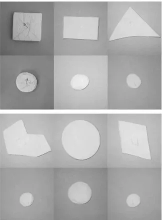
FIG. 8: Typical shapes of Mont St.-Michel rip-up clasts. The immature pebbles in the top row were collected close to their origin; the sub-mature pebbles in the middle row were col-lected further downstream; the smooth, mature pebbles in the bottom row were collected on a nearby sandbar. As these pebbles eroded, their shapes became rounder, an effect quan-tified in the next figure. The bars indicate, in each row, a length of 2 cm.

sub-mature pebbles found further “downstream”. As a result of erosion, these pebbles are smaller and smoother than the cobble. Thirty five samples were examined; for these, the average perimeter is 180 mm. The third class is rounded, mature pebbles found on a nearby sand bar. The relation of these pebbles to the other two classes is not clear. Seventeen samples were examined; for these, the average perimeter is 220 mm.

Typical photographs for each of these classes are shown in Fig. 8. The average of the cumulative curvature distri-bution for all samples in each class is shown in Fig. 9. The angularity of the large cobble is reflected in the breadth of the curvature distribution. Roughly a quarter of the perimeter has negative curvature, and roughly a tenth has curvature five times greater than the average. For the other two classes, the curvature distribution is pro-gressively more narrow. The relative steepness of the f (K)’s shows that all of these shapes are less round than the final pebbles produced by the laboratory erosion ma-chine.

The width of the curvature distribution can be speci-fied quantitatively by the standard deviation, σ. Results are normalized by the average curvature, and are shown for the field and laboratory pebbles in Table I. The peb-bles with steeper f (K) indeed have smaller widths. For example, the width for the immature field cobble is about 3-4 times that of the average laboratory pebble. While the dimensionless width of the distribution, σ/hKi, is a useful number for comparisons, it does not distinguish between curvature distributions of different shape. The actual functional form of the curvature distribution can be specified to some extent by comparing its moments with that of a Gaussian. In particular, the “skewness” and “kurtosis” are dimensionless numbers defined by the

7 1 0.8 0.6 0.4 0.2 1 - 2 0 2 4 6 8 sub-mature immature mature laboratory average f(K) K/<K>

FIG. 9: (Color online) Cumulative curvature distribution, f (K), for the average shapes of Mont St.-Michel rip-up clasts. Even the roundest shapes remained less circular than the final shape in the laboratory study.

third and fourth moments, respectively, in such a way as to vanish for a perfect Gaussian. The results in Table I show that the four classes of pebbles have curvature dis-tributions of four distinct forms. Of these, the laboratory pebbles are closest to a Gaussian.

Note that the curvature distribution data show no ev-idence of a stationary shape, in which the clasts erode away without changing shape. Rather, the three classes of clasts all have different sizes and shapes. Thus it would not be fruitful to compare or fit the clast erosion to the cutting model we introduced in Ref. [8]. However, since the sub-mature and mature clasts are smaller than the immature clasts but are not circular, we can rule out the polishing model.

Class Perimeter (mm) σ/hKi Skewness Kurtosis immature 550±100 2.4±0.3 1.4±0.3 3.8±1.4 sub-mature 180±60 2.0±0.6 0.0±0.9 3.3±2.9

mature 220±70 1.4±0.3 -0.2±0.5 1.3±1.0

lab-final 122±25 0.8±0.1 0.1±0.5 1.0±1.5

TABLE I: Characteristics of curvature distribution for the three classes of field pebbles. Final laboratory pebble shape is added for comparison.

V. CONCLUSION

We have studied the formation of two-dimensional peb-ble shapes. As in Ref. [8] we introduced a local descrip-tion of the erosion process, based on the distribudescrip-tion function of the curvature, measured along the pebble con-tours. This description captures both the local character of the erosion events, and the statistical nature of the erosion process.

For pebbles generated in the laboratory, we have shown that the curvature distribution has two important prop-erties. First, the erosion drives the distribution towards

a stationary form. When this stationary state is reached, the pebble contour still changes but, within small fluc-tuations, its curvature distribution remains the same, provided that the curvature is normalized by its average value. Secondly, we have found that the final stationary form of the distribution is independent of the original pebble shapes. This not only shows that the curvature distribution is a property of the erosion process itself, but it also opens the interesting possibility of establishing a classification of different erosion processes according to the type of curvature distribution they generate.

For pebbles collected in the field, we have made a first attempt to study a special class of rip-up clasts from the St.-Michel bay. These mud pebbles can be collected at very different erosion stages within a relatively small area of the tidal flats. We showed that the curvature distribution sharpens with the wearing degree, without getting however as sharp as the distribution obtained in the laboratory experiments.

The results presented in this experimental paper sug-gest a number of directions for modeling the formation of flat pebbles. Of central importance is the intrinsic statis-tical nature of the erosion process itself. As first hinted in Ref. [8], a sequence of cuts of a noiseless, deterministic nature typically leads to a trivial curvature distribution like that of a circle. We also demonstrated in Ref. [8] that a “cutting” simulation, with an appropriate distrib-ution of cutting lengths, acting most strongly on regions of high curvature in accord with Aristotle’s intuition [1], can reproduce the curvature distribution from the lab-oratory experiments. We will address these and other questions relevant for the theoretical modeling of pebble formation in a forthcoming paper.

Acknowledgments

We acknowledge insightful discussions with F. Thal-mann and experimental insight by P. Boltenhagen. This work was supported by the Chemistry Department of the CNRS, under AIP “Soutien aux Jeunes Equipes” (CM). It was also supported by the National Science Foundation under Grant DMR-0514705 (DJD).

APPENDIX: CURVATURE ANALYSIS

The goal of this section is to provide a detailed, prac-tical description of two means to measure the local cur-vature at each point along the pebble contour. In both cases the starting point is an image of the pebble. For our work we use a digital camera Canon Power Shot G1 with a resolution of 1024 × 768 pixels. It should be just as effective to scan conventional photographs, or even to scan pebbles themselves. To determine the {x,y} coor-dinates of the contour, we import the images into NIH Image [32], which includes routines for finding edges and for skeletonizing the result. An example of the digitized

pebble contour, and the smooth reconstructions to be dis-cussed below, is given in Fig. 10. We show the contour in pixel units, since the actual calibration is needed only to determine size, not shape. Note from the inset that the contour points are indeed pixelized and skeletonized, with each point having only two neighbors located at ei-ther ±1 or 0 units away in the x- and y-directions. If the digitization process is faithful, then the uncertainty in each pixel is about ±0.5 units in each direction. This is not small compared to the distance between neighboring pixels, so a smoothing or fitting routine is necessary to reconstruct the actual contour and thereby extract the curvature distribution.

To illustrate the difficulties of extracting curvature, let us begin with two methods that are, in fact, unsatis-factory. It is perhaps tempting to simply smooth the data, replacing each point with a weighted average of neighbors lying within some window. Weights could be cleverly chosen to de-emphasize points at the edge of the window, for example. This fails, however, since it’s far from obvious how to choose a suitable window size. For instance, the pixelized representation of the straight sec-tion given by y = 0.1x for 0 < x < 10 is a step funcsec-tion y = 0(1) for x < (>)5. A large window would be needed to even approximately reconstruct the original line. How-ever, such a sufficiently large smoothing window would erase fine features if applied elsewhere along the contour. Since smoothing filters provide no feedback on quality, vi-sual inspection of the result would be necessary to choose an optimal window size at each point along the contour. This is not only subjective, but rather impractical. As an alternative, it is perhaps tempting to implement an automated version of Wentworth’s curvature gauge [9]. This is a device with circular notches of various diam-eters into which portions of a pebble may be pressed. The computational analogue would be to find the best nonlinear-least-squares fit to a circle at each point along the pebble contour. As with smoothing, one difficulty is to find the optimal window over which to do the fitting. A compounding difficulty is that essentially nowhere is the pebble exactly circular, so even with ‘the’ optimal window there is substantial disagreement between data and fit. A spectacular example of this problem is at an inflection point, where the curvature changes from posi-tive to negaposi-tive.

To overcome such difficulties, we propose to fit digi-tized contour data to a cubic polynomial at each point along the contour. A cubic is the lowest order polynomial needed in order to avoid systematic error when the cur-vature varies gradually across the fitting window, which is the usual case. In order to avoid having to rotate the coordinate system to ensure that the contour y(x) is a single-valued function, we instead convert to polar coordinates. Thus we define the origin by the center-of-mass of the contour and perform fits to r(θ) where r =px2_{+ y}2 _{and θ = tan−1(y/x). Once a satisfactory}

fit is achieved, the curvature may be deduced from the

-200 -150 -100 - 5 0 0 5 0 1 0 0 1 5 0 2 0 0 -200 -150 -100 - 5 0 0 5 0 1 0 0 1 5 0 2 0 0 - 1 6 0 - 1 5 0 - 1 4 0 - 1 3 0 - 1 2 0 - 1 1 0 1 0 0 1 1 0 1 2 0 1 3 0 1 4 0

FIG. 10: (Color online) Reconstruction of a smooth pebble contour from the pixelized digital representation. The solid curve is based on fitting to cubic polynomials at each point. The dashed curve is based on the iteration scheme of Fig. 11.

value and derivatives of the cubic polynomial by K = r 2 + 2r2 θ− rrθθ (r2_{+ r}2 θ) 3/2 , (A.1) where rθ= dr/dθ and rθθ= d2r/dθ2[30].

Two tricks seem necessary to achieve satisfactory re-sults. The first is to weight the data most heavily near the center of the window. We use a Gaussian weighting function with a standard deviation equal to 1/4 of the width of the window. This ensures that points at the edges have essentially no influence. Therefore, the fitting results do not vary rapidly as the window is slid along the contour. This guarantees that the reconstructed curve and its first two derivatives are continuous, which is a crucial requirement for measuring the curvature.

The second trick is to choose the window size appro-priately. This is actually the most difficult and subtle aspect of the whole problem. If the window is too small, then the fit will reproduce the bumps and wiggles of the pixelization process; usually the curvature will be over-estimated. If the window is too large, then the fit will significantly deviate from the data; usually the curvature will be underestimated. And while the curvature tends to decrease systematically with window size, there is in general, unfortunately, no plateau between these two ex-tremes where the curvature is relatively independent of window size and hence clearly represents the true value. To pick the window appropriately requires careful un-derstanding of the numerical fitting procedure and the feedback it provides. Since the fitting function is a poly-nomial, the minimization of the χ2

total square deviation from the data reduces to solving a set of linear equations. This in turn reduces to inverting a matrix. If the window is too small then the fit will be ‘ambiguous’ in the sense

9 that χ2

is small but the error in the fitting parameters is large. Mathematically, the matrix to be inverted is essen-tially singular. A good strategy is therefore to start with a small window and increase its size until the matrix is no longer singular. This can be accomplished using a lin-ear least-squares fitting routine based on singular-value decomposition [31]. However, the uncertainty in fitting parameters for the first suitable window is generally too large (nearly 100%). So we increase the window size two pixels at a time until the error in curvature has been re-duced by a factor of ten. This defines the largest suitable window, beyond which systematic errors due to incorrect functional form begin to appear. We have not been able to define the largest suitable window based on the value of χ2

. For the final result, we take a weighted average of the cubic fit parameters over all suitable windows, where the weights are set by the uncertainties in fitting para-meters as returned by the fitting routine. An example of a reconstructed contour from this procedure is shown by the solid curve in Fig. 10. The recontruction is sat-isfactorily smooth; also, it clearly avoids the pixel noise without smoothing over significant small-scale features in the contour.

Since the cubic fitting method is rather involved, and since the choice of window sizes is still slightly subjective, we have developed an alternative method. The starting point is the fact that the actual digital representation of the contour depends on the location and orientation of the pebble with respect to the grid of pixels. If the pebble were shifted or rotated, then the pixelized repre-sentation would be slightly different. For example, imag-ine the pixelization of a limag-ine making various angles with the grid. Perhaps the ideal experimental measurement procedure would be to systematically reposition the peb-ble, pixelize, then compute the average of all such rep-resentations. However this procedure does not lend it-self to automatization, and would be impractically time-consuming. Instead, we propose to do more or less the same thing numerically. The idea is to take the current best guess for the contour, pixelize it with respect to a random grid position and orientation, then use the new representation to update the best guess. When iterated, this procedure converges to a satisfactory reconstruction

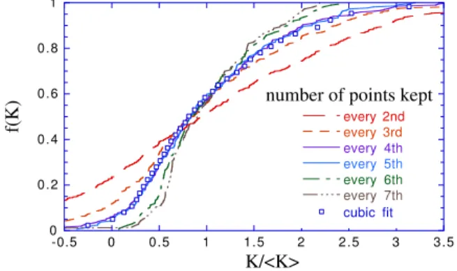
of the actual contour with two provisos. First, at each step, we locally smooth the trial pixelization by replacing each point by its average with its two immediate neigh-bors. Second, we keep only every fourth or fifth point in the original pixelized data and perform all operations on this subset. When done, we compute the curvature literally by the change of slope with respect to arclength using the straight segments between adjacent points.

The cumulative curvature distribution given by this it-eration scheme is shown in Fig. 11 as a function of the number of points kept. When too many are kept, the re-constructed curve follows the bumps and wiggles of the original pixelization too closely; the curvature distribu-tion is too broad. When too few are kept, the recon-structed curve incorrectly smooths over small-scale

fea-1 0.8 0.6 0.4 0.2 0 -0.5 0 0.5 1 1.5 2 2.5 3 3.5 cubic fit every 2nd every 3rd every 4th every 5th every 6th every 7th f(K) K/<K>

number of points kept

FIG. 11: (Color online) Trial integrated curvature distribu-tions from the iterative smoothing scheme, vs the number of points kept. Keeping either 4 or 5 points seems optimal: the resulting distributions are identical and they agree with that based on cubic fits.

tures; the curvature distribution is too narrow. When only every fourth or fifth point are kept, the distributions are nearly equal; furthermore, they are indistinguishable from that given by the cubic polynomial fitting. The ac-tual reconstructed contour is also shown in Fig. 10. The plateau in the curvature distribution vs number of points kept, and the good agreement with the other method, both give confidence in this new iterative reconstruction scheme.

[1] Aristotle, Minor Works, Mechanical Problems (Harvard University Press, Cambridge, 2000), translation by W.S. Hett. Question 15 asks: “Why are the stones on the seashore which are called pebbles round, when they are originally made from long stones and shells? Surely it is because in movement what is further from the middle moves more rapidly. For the middle is the center, and the distance from this is the radius. And from an equal movement the greater radius describes a greater circle. But that which travels a greater distance in an equal time describes a greater circle. Things travelling with a greater velocity over a greater distance strike harder, and

things which strike harder are themselves struck harder. So that the parts further from the middle must always get worn down. As this happens to them they become round. In the case of pebbles, owing to the movement of the sea and the fact that they are moving with the sea, they are perpetually in motion and are liable to fric-tion as they roll. But this must occur most of all at their extremities.”.

[2] Lord Rayleigh, F.R.S., Nature 3901, 169 (1944). [3] S. Boggs, Jr., Principles of sedimentology and

stratigra-phy (Prentice Hall, N.J., 2001), 3rd ed.

Con-densed Matter Physics (Cambridge University Press, New York, 1995).

[5] R. Lipowsky and E. Sackmann, Structure and dynamics of membranes, Handbook of biological physics (Elsevier, Amsterdam, 1995).

[6] P. Meakin, Fractals, scaling and growth far from equilib-rium (Cambridge University Press, Cambridge, 1998). [7] B. Jamtveit and P. Meakin, eds., Growth, dissolution and

pattern formation in geosystems(Kluwer Academic Pub-lishers, Dordrecht, 1999).

[8] D. J. Durian, H. Bideaud, P. Duringer, A. Schroder, F. Thalmann, and C. M. Marques, Phys. Rev. Lett. 97, 028001 (2006).

[9] C. K. Wentworth, Journal of Geology 27, 507 (1919). [10] H. Wadell, Journal of Geology 40, 443 (1932).

[11] W. C. Krumbein, Journal of Sedimentary Petrology 11, 64 (1941).

[12] W. C. Krumbein, Journal of Geology 49, 482 (1941). [13] A. Cailleux, C. R. Soc. Geol. Fr. Paris 13, 250 (1947). [14] G. G. Luttig, Eizeitalter u. Gegenwart (Ohningen) 7, 13

(1956).

[15] M. Blenk, Z. Geomorph. Berlin NF 4 3/4, 202 (1960). [16] P. H. Kuenen, Geol. Mijnbouw (Leiden) 44, 22 (1965). [17] P. Duringer, Th`ese de doctorat detat, Universit´e Louis

Pasteur (1988).

[18] E. D. Sneed and R. L. Folk, Journal of Geology 66, 114 (1958).

[19] W. K. Illenberger, Journal of Sedimentary Petrology 61,

756 (1991).

[20] D. I. Benn and C. K. Ballantyne, Journal of Sedimentary Petrology 62, 1147 (1992).

[21] J. L. Howard, Sedimentology 39, 471 (1992).

[22] H. J. Hofmann, Journal of Sedimentology Research 64, 916 (1994).

[23] D. J. Graham and N. G. Midgley, Earth Surface Processes and Landforms 25, 1473 (2000).

[24] H. P. Schwarcz and K. C. Shane, Sedimentology 13, 213 (1969).

[25] R. Ehrlich and B. Weinberg, Journal of Sedimentary Petrology 40, 205 (1970).

[26] M. W. Clark, Journal of the International Association for Mathematical Geology 13, 303 (1981).

[27] M. Diepenbroek, A. Bartholoma, and H. Ibbeken, Sedi-mentology 39, 411 (1992).

[28] E. T. Bowman, K. Soga, and W. Drummond, Geotech-nique 51, 545 (2001).

[29] H. Drolon, F. Druaux, and A. Faure, Pattern Recognition Letters 21, 473 (2000).

[30] E. W. Weisstein, The CRC concise encyclopedia of math-ematics(CRC Press, New York, 1999).

[31] W. H. Press, B. P. Flannery, S. A. Teukolsky, and W. T. Vetterling, Numerical Recipes in C (Cambridge Univer-sity Press, New York, 1992), 2nd ed.

[32] NIH Image, public domain software available at http://rsb.info.nih.gov/nih-image/.