HAL Id: insu-02887149
https://hal-insu.archives-ouvertes.fr/insu-02887149
Submitted on 4 Jan 2021HAL is a multi-disciplinary open access archive for the deposit and dissemination of sci-entific research documents, whether they are pub-lished or not. The documents may come from teaching and research institutions in France or abroad, or from public or private research centers.
L’archive ouverte pluridisciplinaire HAL, est destinée au dépôt et à la diffusion de documents scientifiques de niveau recherche, publiés ou non, émanant des établissements d’enseignement et de recherche français ou étrangers, des laboratoires publics ou privés.
Gianluca Carnielli, Marina Galand, François Leblanc, Ronan Modolo, Arnaud
Beth, Xianzhe Jia
To cite this version:
Gianluca Carnielli, Marina Galand, François Leblanc, Ronan Modolo, Arnaud Beth, et al.. Sim-ulations of ion sputtering at Ganymede. Icarus, Elsevier, 2020, 351 (November), pp.113918. �10.1016/j.icarus.2020.113918�. �insu-02887149�
Simulations of ion sputtering at Ganymede
G. Carnielli, M. Galand, F. Leblanc, R. Modolo, A. Beth, X. Jia
PII: S0019-1035(20)30296-7
DOI: https://doi.org/10.1016/j.icarus.2020.113918
Reference: YICAR 113918
To appear in: Icarus
Received date: 22 August 2019 Revised date: 5 April 2020 Accepted date: 8 June 2020
Please cite this article as: G. Carnielli, M. Galand, F. Leblanc, et al., Simulations of ion sputtering at Ganymede, Icarus (2018),https://doi.org/10.1016/j.icarus.2020.113918
This is a PDF file of an article that has undergone enhancements after acceptance, such as the addition of a cover page and metadata, and formatting for readability, but it is not yet the definitive version of record. This version will undergo additional copyediting, typesetting and review before it is published in its final form, but we are providing this version to give early visibility of the article. Please note that, during the production process, errors may be discovered which could affect the content, and all legal disclaimers that apply to the journal pertain.
Journal Pre-proof
Simulations of ion sputtering at Ganymede
G. Carniellia,*, M. Galanda, F. Leblancb, R. Modoloc, A. Betha, X. Jiad a
Department of Physics, Imperial College London, SW7 2AZ, London, United Kingdom
b
LATMOS/IPSL, CNRS, Sorbonne Université, UVSQ, Paris, France
c
LATMOS/IPSL, UVSQ Université Paris-Saclay, UPMC Univ. Paris 06, Guyancourt, France
d
Department of Climate and Space Sciences and Engineering, University of Michigan, Ann Arbor, MI 48109-2143, USA
*Principal corresponding author:
Email address: [email protected] (G. Carnielli)
Abstract
Ganymede‟s surface is subject to constant bombardment by Jovian magnetospheric and Ganymede‟s ionospheric ions. These populations sputter the surface and contribute to the replenishment of the moon‟s exosphere.
Thus far, estimates for sputtering on the moon‟s surface have included only the contribution from Jovian ions. In this work, we have used our recent model of Ganymede‟s ionosphere (Carnielli et al., 2019) to evaluate the contribution of ionospheric ions for the first time. In addition, we have made new estimates for the contribution from Jovian ions, including both thermal and energetic components.
For Jovian ions, we find a total sputtering rate of 2.2 10 27 s1
, typically an order of magnitude higher compared to previous estimates. For ionospheric ions, produced through photo- and electron-impact ionization, we find values in the range 2.7 10 26 – 5.2 10 27 s1 when the moon is located above the Jovian plasma sheet. Hence, Ganymede‟s ionospheric ions provide a contribution of at least 10% to the sputtering rate, and under certain conditions they dominate the process. This finding indicates that the ionospheric population is an important source to consider in the context of exospheric models.
Keywords: Ganymede, Ionospheres, Jupiter, satellites, Satellite, atmospheres
1. Introduction
Besides sublimation, ion bombardment of Ganymede‟s surface, leading to sputtering, has long been identified as a key source of the moon‟s neutral exosphere (Pilcher, 1976; Lanzerotti et al., 1978; Johnson, 1990). In this work, we refer to sputtering as the ejection of all neutral species from the icy surface, including those formed within the surface through different chemical paths following water radiolysis, such as H2 and O2. Sources of impactors include primarily ions from the Jovian magnetosphere and from Ganymede‟s ionosphere, with electrons supposedly providing only a small contribution (Galli et al., 2017). The thermal Jovian magnetospheric plasma at the moon‟s orbital distance is populated by O and H ions, as determined by the PLasma Science (PLS) instrument on board Galileo (Frank et al., 1997; Neubauer, 1998). The energetic component has been probed by the Energetic Particle Detector (EPD) and includes H,
Journal Pre-proof
On and Sn ions (Cooper et al., 2001; Mauk et al., 2004). Unlike the Jovian magnetospheric plasma, the composition of Ganymede‟s ionosphere is poorly constrained from observations; according to our recent ionospheric model, the ionospheric population includes primarily O2 ions, followed by O , H 2O
, H 2
, H and OH (Carnielli et al., 2019). All the above-mentioned ion species impact the moon‟s surface and contribute to the sputtering process.
Quantifying the sputtering process requires knowledge of how the plasma impacts the surface in terms of spatial distribution of the impact flux and impact energy, as well as of the sputtering yield, i.e., the number of atoms or molecules ejected per impacting ion. The yield depends on several parameters, including the surface composition, temperature, impacting species‟ mass, energy and angle of incidence, and can be found empirically. However, experiments cannot faithfully replicate the physical conditions on Ganymede‟s surface, especially in regards to the detailed surface composition at the microscopic level, which matters for the sputtering process. As a result, actual yields at Ganymede could differ from the analytic fits found empirically to estimate sputtering on icy moons and reported in the literature, including those from Johnson (1990), Shi et al. (1995), Johnson et al. (2004), Famá et al. (2008), Johnson et al. (2009), and Teolis et al. (2017).
The sputtering contribution from Jupiter‟s magnetospheric ions has been estimated in different ways. Shi et al. (1995) made the first estimate by combining the sputtering yield compiled from experiments and an estimate of the impact rate only of thermal Jovian plasma, without considering Ganymede‟s own magnetic field, which was unknown at the time. As a result, they assumed Jovian ions impacting only on the ram hemisphere, obtaining a value of 1.70 10 28 s1
. Ip et al. (1997) made use of the energetic ion fluxes (in the energy range 0.1–104
keV) measured by the EPD instrument when Galileo was inside the Alfvén wings during the G2 flyby, and had it uniformly impact the polar regions, assuming no change in the flux distribution; using the energy-dependent sputtering yields compiled by Johnson (1990) they obtained a total rate of
26
1.01 10 s1. Paranicas et al. (1999) took the same approach of Ip et al. (1997) using a combination of sputtering yields from Johnson (1990) and Shi et al. (1995), and EPD data (approximately in the range 0.5–3000 keV) from the G7 flyby. Assuming sputtering to take place in the polar caps, approximated by the surface area above 45 , they estimated a rate of 2 10 26 s
1
. Cooper et al. (2001) ran a simulation using EPD data from the G2 encounter (in the energy range 20–105
keV) for the energetic Jovian plasma, and simulated test particles with a backward tracing technique. Using the yields from Shi et al. (1995) they estimated a total sputtering rate of
28
4.33 10 s1
. Plainaki et al. (2015) simulated the impact of both thermal and energetic Jovian ions using a test particle approach, cutting at 125 keV the simulation for energetic ions. They estimated the sputtering rate using the analytic expressions derived by Famá et al. (2008) and Johnson et al. (2009) for the energy- and species-dependent sputtering yields. They calculated a total sputtering rate of 6.94 10 25 s1, i.e., more than one order of magnitude lower compared to previous estimates. Finally, the most recent estimate, from Poppe et al. (2018), was obtained from backward-tracing test particle simulations of thermal ions approximately in the energy range 102–10 keV and energetic ions in the range 1–105 keV. Using the analytic fit of Johnson et al. (2004) for the sputtering yield, they calculated a total rate of 7.5 10 26 s1.
These estimates do not give a complete account of the sputtering taking place on the moon‟s surface as the ionospheric contribution has been neglected. In this work, we present the results of the first estimate of the contribution from ionospheric species as well as new estimates
Journal Pre-proof
for Jovian magnetospheric thermal and energetic ions.
The paper is organized as follows. Section 2 outlines the methods used to simulate the contribution from each ion population. In Section 3 we present the results of the contribution from each species and compare our findings with previous works in regards to the Jovian ion population. In Section 4 we discuss the implication of the results presented in Section 3. Finally, Section 5 summarizes the results obtained in this work.
2. Methods
2.1. Test-particle model
Our calculations rely on the test-particle code described in Carnielli et al. (2019). All results shown in this work derive from simulations driven by the electric and magnetic fields obtained from the MHD model of Jia et al. (2009) for the G2 flyby conditions. The fields are defined on a cubic grid of size 20 RG20 RG20 RG (corresponding also to the size of the simulation volume), centred on Ganymede, with a spatial resolution of 0.05 RG.
At the moon‟s surface, a spherical grid of 90180 cells with angular separation of 2 in the latitudinal and longitudinal directions collects the impact rate and impact energy of each test particle. The sputtering rate is calculated by multiplying the impact rate by Y, the energy-dependent sputtering yield. For the latter, we used the expressions of Famá et al. (2008) for impact energies < 100 keV and of Johnson et al. (2009) for higher impact energies:
/ 2 1 0 2 0 0 1 2.8 1/3 2.16 2.8 1/3 2.24 3 1/ 1 cos ( ), < 100 keV 4 = 1/ (4.2 [ / ] ) 1/ (11.22 [ / ] ) , 100 keV Ea k TB f n e Y U S S e E C Y Y Z v Z Z v Z E (1)where the dependence on the impacting energy E comes from various terms within the equation.
is the angle of incidence of the impacting ion (0 = normal to the surface) and T is the surface temperature. For a more detailed explanation of all other terms, see Famá et al. (2008) and Johnson et al. (2009). For the surface temperature we used the same distribution as in Leblanc et al. (2017), with a minimum temperature of 80 K in the night side and a peak of 150 K at the subsolar point. The test particle code potentially allows to calculate exactly the angle of incidence of test particles with respect to the surface. However, Ganymede‟s surface is not perfectly spherical. The surface is grooved, thus one cannot predict precisely the angle of incidence of the impacting particle with respect to the section of surface intersected in the collision. Therefore, for each impact we assumed an incidence angle of 45 , corresponding to the average amongst the possible values between 0 and 90 . In a similar way compared to the sputtering rate, we calculated the sputtering flux by multiplying the impact flux by the energy-dependent sputtering yield.
2.2. Simulation setup for thermal Jovian ions
The MHD model of Jia et al. (2009) assumed a single-species plasma with an average mass density of 28 AMU cm3 for the G2 flyby conditions. Assuming a mean ion mass of 13 AMU (Neubauer, 1998) and an electron number density in the range 1–5 cm3 (reported by Kivelson et al. (2004)), it follows that O dominates the plasma composition, as also reported from observations (Frank et al., 1997). We ran test simulations for thermal H, which is still an
Journal Pre-proof
important source of Jovian plasma at Ganymede‟s orbital distance (Kivelson et al., 2004); we found that thermal H is mostly diverted around the moon due to its low inertia, and that its contribution to the impact and sputtering flux is negligible. Hence, in the test-particle simulations of the thermal Jovian plasma we assumed the species to be O with a number density of 1.75 cm
3
at the simulation boundary, i.e., outside Ganymede‟s magnetosphere. We describe this population with a Maxwellian distribution with a temperature of 360 eV (Neubauer, 1998). To be consistent with the initial conditions in the model of Jia et al. (2009), the mean speed is set to 140 km/s – the near-corotation speed – in the corotation direction and 0 km/s in the perpendicular directions.
Hard boundary conditions are applied, meaning that particles are not allowed to be reflected at the boundaries. Periodic boundary conditions are not applicable because that would imply that ions are able to mirror in the Jovian magnetosphere quickly enough to interact twice with Ganymede‟s magnetosphere, while the mirroring time significantly exceeds the transit time of the flux tube across the moon‟s surface.
2.3. Simulation setup for energetic Jovian ions
The energetic component of the Jovian magnetospheric plasma is populated by H, On and Sn
ions (Cooper et al., 2001; Mauk et al., 2004), and in the proximity of Ganymede it has been characterized to some extent by the Energetic Particle Detector (EPD) on board the Galileo spacecraft. The energy spectra of all energetic species near Ganymede (but outside its magnetosphere) recorded at the time of the G2 flyby have been published by Cooper et al. (2001) and Mauk et al. (2004).
In our simulations, we have used the analytical fits reported in Mauk et al. (2004) – in the energy range from 20 keV to 30 MeV – to simulate the injection flux at the boundaries of the simulation box, assuming a charge state of q= 2 for atomic oxygen and q= 3 for atomic sulphur (Keppler and Krupp, 1996). As the energy range spans three orders of magnitude, it is not feasible to run a simulation that injects test particles across the whole energy range with sufficient statistics. For this reason, we have divided the energy spectrum of each species into 10 equally spaced bins (in logarithmic scale), each of which having an average value for the intensity within the given energy range. In other words, for each ion species we ran 10 different simulations, each one simulating a different energy range. This ensures that the whole energy spectrum is correctly represented with sufficient statistics. Hence, a total of 30 simulations were carried out to simulate the full energy spectrum for all simulated energetic ion species.
Test particles were initialized with a random velocity direction, a random energy within the energy bin and a weight determined by the mean intensity. While for the thermal population the motion is predominantly in the corotation direction, for energetic ions the corotation flow speed – approximately 140 km/s in Ganymede‟s frame of reference – contributes negligibly (a few keV) to the ion‟s kinetic energy, hence the injection flux is uniform across all boundaries of the simulation box. Like for thermal Jovian ions, hard boundary conditions are applied since the mirroring time in the Jovian magnetosphere vastly exceeds that of convection through Ganymede‟s magnetosphere. The timestep is calculated at each iteration ensuring that the test particle does not skip cells and does not travel more than 1/20th of the local gyro-radius.
2.4. Simulation setup for ionospheric ions
Journal Pre-proof
exosphere obtained from the model of Leblanc et al. (2017), and ionized it via photo- and electron-impact ionization. The ion species simulated are O2, O, H2O, H2, H, and OH. The reader is referred to Table 2 in Carnielli et al. (2019) for the list of ionization frequencies used and to the same paper for a more detailed discussion of these simulations in regards to the assumptions made.
3. Results
3.1. Jovian ions
Figure 1: Surface maps of the impact flux (top row), average impact energy (middle row) and sputtering flux (bottom row) for Jovian thermal O (first column), energetic H (second
column), O2 (third column) and S3 (fourth column). The boundaries between open and closed magnetic field lines are plotted in black. 0 longitude corresponds to the bisector of the leading hemisphere and 90 is toward Jupiter. Note that color scales differ also between plots in the same row.
Figure 1 shows surface maps of the impact flux, impact energy, and sputtering flux for Jovian thermal and energetic ions. For thermal O (first column in Figure 1), the map appears patchy in the polar regions because of statistics, which is insufficient to generate a comprehensive mapping of the impact process. The simulation was launched with 3.2 10 8 particles. However, only around 950,000 (less than 1%) test particles impacted the surface, explaining the patchy appearance. Nonetheless, we do not expect that a refined statistics would change the conclusions from our study. The impact concentrates primarily near the separatrix region (black, solid lines), but is also present in the equatorial region of the leading hemisphere and, to a much smaller extent, in the polar regions. The ions impacting in the polar regions and close to the equator originate inside the Alfvén wings or at their boundaries. They move along the magnetic field lines and accelerate nearby the moon before impacting the surface. Instead, thermal ions impacting near the separatrix are primarily produced outside the wings, and mainly originate at the upstream boundary plane of the simulation box, where plasma inflow is strongest.
For the impact energy, there is a clear distinction between the equatorial region in the leading hemisphere and the polar regions. At the poles, thermal ions move slowly due to the low electric field intensity found by the MHD model, and impact „gently‟ on the surface, with typical energies of the order of 10–100 eV. Instead, at low latitudes in the wake hemisphere impacts occur with energies equal or greater than their initial energy (1–6 keV). These are thermal ions that accelerate along the surface boundary of the Alfvén wings. This means that the bulk Jovian plasma is more efficient at sputtering near the separatrix and in the wake hemisphere at low latitudes as sputtering is more efficient at high impact energies. As a result, the sputtering is concentrated near the separatrix and at low latitudes in the wake hemisphere, instead of the polar regions, as seen in the bottom panel of the first column.
The second, third and fourth columns in Figure 1 show the impact flux, impact energy and sputtering flux for the energetic population. The maps for each species combine the results from 10 simulations, each of which assessing a different energy range (see Section 2.3). In terms of impact
Journal Pre-proof
flux (top row), the maps look different for each species. For H, the majority of impact occurs in the polar regions, where magnetic field lines are open. This is due to the ion‟s low inertial mass, which limits significantly its ability to penetrate inside the closed magnetic field line region. However, for O2
and S3
this is not the case. For O2
, the higher mass-to-charge ratio leads to a partial penetration inside the equatorial region, but the impact still concentrates mainly near the separatrix line in both hemispheres. For S3
, as the magnetic shielding is less efficient for this heavy species (compared to the lighter ones), the penetration at low latitudes is enhanced, as seen by the more orange/red color in this region. Therefore, for S3
a larger fraction of the impact occurs in the equatorial region.
The maps of impact energy (middle row) show the opposite case compared to the impact flux. The average impact energy, for all species, is greatest in the equatorial region. This duality is most visible for H, whose average impact energy at the poles is everywhere around 10 keV, while in the closed field lines region it is almost everywhere between 0.1–1 MeV. This trend is explained by the fact that only ions with a relatively high energy are able to penetrate the closed field lines. Note, the duality is seen less with heavier ions, i.e., O2 and S3, as the inertial mass eases the penetration at low latitudes. Also note, energetic ion impact occurs also in the polar regions, but the ion intensity decreases exponentially with increasing energy, therefore the average impact energy is still low.
The sputtering maps (bottom row) show the combination of impact flux and average impact energy. Overall, the maps look similar to those of the impact flux, but the gap between polar and equatorial regions is less pronounced due to the larger sputtering yield in the equatorial region, associated with the larger impact energy. For H, most of the sputtering still occurs in the polar regions, while for S3
it occurs mostly in the equatorial region. For O2
, it is highest near the separatrix between open and closed field lines.
Figure 2: Impact (top) and sputtering (bottom) fluxes as a function of impact energy for different Jovian ion species: O from the thermal population (gold), energetic H (red), energetic O2 (green) and energetic S3 (blue). Each data point corresponds to the total flux over the energy range delimited by the adjacent vertical lines. The solid curves show values in the region of open magnetic field lines (north and south combined together), while the dashed lines show values in the region of closed magnetic field lines.
Figure 2 shows the impact (top) and sputtering (bottom) fluxes for each Jovian species as a function of energy, including the thermal (yellow curves) and energetic populations (H in red, O
2
in green and S3 in blue). The solid line shows values in the region of open magnetic field lines, which includes the northern and southern polar regions, while the dashed line shows values in the closed magnetic field lines region. Each data point represents the total flux integrated over the energy range delimited by the surrounding vertical lines.
In terms of impact flux, H dominates in the polar regions for energies above a few hundreds of eV, while thermal O dominates at lower energies. In the equatorial region, thermal O dominates up to 1 keV, while at higher energies the energetic species more or less equally contribute to the impact flux. For these energetic species, the peak impact flux in the polar regions occurs at approximately 10 keV, and at this energy is roughly the same compared to the equatorial
Journal Pre-proof
region (except for H, for which the impact flux in the equatorial region is one order of magnitude lower). At higher energies, the profiles for the two regions converge, as the shielding effect from the closed field lines becomes irrelevant for the ion dynamics. For thermal O, the peak impact flux is found at approximately 10 eV in the polar regions and at almost 1 keV in the equatorial region. Inside the Alfvén wings, i.e., in the polar regions, the electric field intensity is low, and ions are slowed down from their convective motion outside Ganymede‟s magnetosphere, in which their energy is a few keV.
In terms of sputtering flux (bottom panel in Figure 2), the energy distribution differs significantly compared to the top panel. In this case, there is a clear distinction between the contribution from each species. Sulphur ions are the most efficient at sputtering the moon‟s surface. In particular, their efficiency peaks around 100 keV, which is the energy range in which the combination of ion intensity and sputtering yield leads to the highest ejection rates. The bottom panel in Figure 2 also highlights the difference between sputtering in the polar and equatorial regions. For the bulk plasma population and energetic H, more sputtering is seen to occur in the polar regions (also visible in the second column in Figure 1). Instead, for O2
and S3
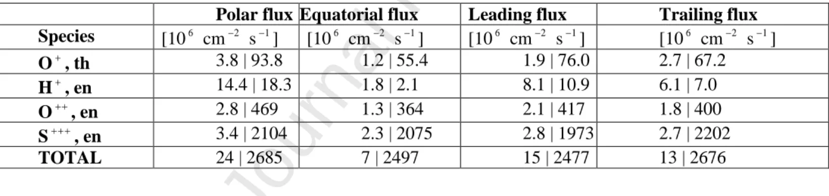
, sputtering in the polar regions dominates only at energies below approximately 10 keV, while at higher energies it takes place mainly in the equatorial region, and is overall highest at low latitudes. Table 1: Fluxes of Jovian thermal („th‟) and energetic („en‟) ions in different regions of Ganymede‟s surface. For each entry, the left and right values correspond to the impact and sputtering flux, respectively. The values shown correspond to the average across the region. For the polar flux, the values are the combined average over the northern and southern polar regions.
Polar flux Equatorial flux Leading flux Trailing flux
Species [106 cm2 s1 ] [106 cm2 s1 ] [106 cm2 s1 ] [106 cm2 s1 ] O, th 3.8 | 93.8 1.2 | 55.4 1.9 | 76.0 2.7 | 67.2 H, en 14.4 | 18.3 1.8 | 2.1 8.1 | 10.9 6.1 | 7.0 O, en 2.8 | 469 1.3 | 364 2.1 | 417 1.8 | 400 S, en 3.4 | 2104 2.3 | 2075 2.8 | 1973 2.7 | 2202 TOTAL 24 | 2685 7 | 2497 15 | 2477 13 | 2676
Table 1 reports more quantitatively the impact and sputtering fluxes of Jovian ions in different regions of Ganymede. “Polar" and “equatorial" indicate, respectively, the regions of open and closed magnetic field lines as found by the MHD model of Jia et al. (2009), with surface areas equal to 3.68 10 17 cm2 and 5.04 10 17 cm2 . “Leading” and “trailing” indicate the respective hemispheres, with both surface areas equal to 4.36 10 17 cm2. In terms of impact flux, there is an overall clear distinction between polar and equatorial regions, with a difference by a factor of more than 3 between the two regions. The asymmetry is driven primarily by energetic H
, which has access dominantly to the open magnetic field line region. Instead, between leading and trailing hemispheres the asymmetry is almost absent, and the small difference is driven by the asymmetric latitudinal extension of the separatrix between open and closed magnetic field lines (see Figure 1), which favors the impact in the leading hemisphere for ions with relatively low energies. In terms of sputtering flux, the asymmetry between polar and equatorial regions almost
Journal Pre-proof
disappears because sputtering is controlled mainly by S3, whose dominant contribution toward sputtering is at high energies, for which the local magnetic field configuration does not matter for the ion‟s trajectory. Like for the impact flux, there is no significant asymmetry between leading and trailing hemispheres either.
Journal Pre-proof
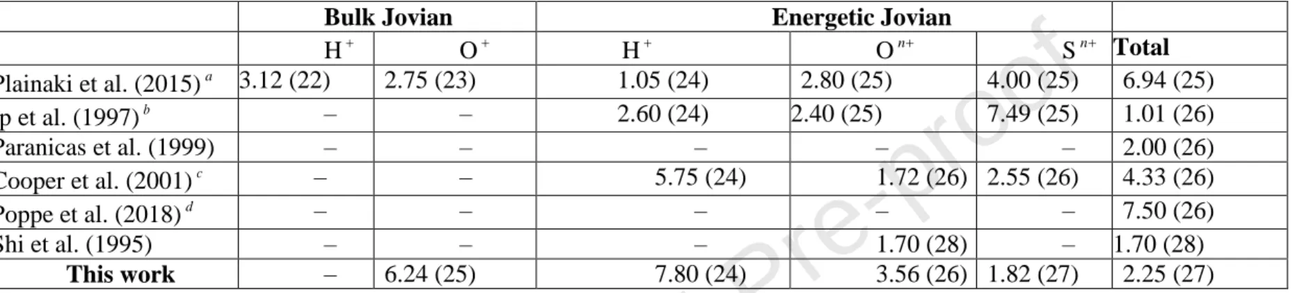
Table 2: Sputtering rates (s1) derived by previously published work and by the test particle code using the fields from the MHD model of Jia et al. (2009) – in which Ganymede is above the Jovian plasma sheet – as input. The number in parentheses indicates the exponent of power 10, e.g., 1.00 (25) corresponds to 1.001025 s1.
Bulk Jovian Energetic Jovian
H O H On Sn Total Plainaki et al. (2015)a 3.12 (22) 2.75 (23) 1.05 (24) 2.80 (25) 4.00 (25) 6.94 (25) Ip et al. (1997)b – – 2.60 (24) 2.40 (25) 7.49 (25) 1.01 (26) Paranicas et al. (1999) – – – – – 2.00 (26) Cooper et al. (2001)c – – 5.75 (24) 1.72 (26) 2.55 (26) 4.33 (26) Poppe et al. (2018)d – – – – – 7.50 (26) Shi et al. (1995) – – – 1.70 (28) – 1.70 (28) This work – 6.24 (25) 7.80 (24) 3.56 (26) 1.82 (27) 2.25 (27) a
Values derived by combining the impact rates of Table 1 and average sputtering yields of Table 2 in Plainaki et al. (2015). b
Values derived from the reported sputtering flux multiplied by the surface area of Ganymede‟s polar regions. c
Values derived by converting the erosion rate (years/mm) in Table 2 of Cooper et al. (2001). d
Journal Pre-proof
The contribution from Jovian ions to sputtering onto Ganymede‟s surface has been previously estimated (see Section 1). Table 2 reports the values obtained from those estimates and from this work. The rates found by our simulations are higher than those found in previous works, except for that of Shi et al. (1995), who likely overestimated the impact flux because they did not consider the presence of Ganymede‟s intrinsic magnetic field. Our results can be compared in more details with Plainaki et al. (2015) and Poppe et al. (2018), who took a similar approach to us in that their estimates are based on test particle simulations.
Plainaki et al. (2015) ran a test particle simulation using the MHD fields of Jia et al. (2009) to simulate both the thermal and energetic components of the Jovian plasma. However, their sputtering rate (which we derived by combining the reported impact rates and energy-dependent sputtering yields) is one order of magnitude lower compared to the one obtained in this work for the case of H and On, and a factor of 30 lower for Sn. Moreover, for all species the impact rate is about one order of magnitude lower (not shown). The discrepancies can be understood considering the different assumptions made in their work: (1) Plainaki et al. (2015) assumed a singly charged state for all ion species, whereas in this work we assumed doubly and triply charged O and S ions, respectively. Different charge-to-mass ratios result in different test-particle trajectories; (2) Plainaki et al. (2015) limited their simulations to ions with energies
100
keV, while in our model we considered ions with higher energies. As shown in Figure 2, S 3
ions with energies > 100 keV account for about half of the sputtering contribution from this species, explaining the greater discrepancy found for S3
. (3) The spatial resolution for the fields in the model of Plainaki et al. (2015) (0.1 RG) is lower compared to that in our model (0.05 RG), which likely has an appreciable effect on the particle dynamics near the surface.
Poppe et al. (2018) simulated the dynamics of Jovian magnetospheric ions in Ganymede‟s environment using a backward-tracing test-particle approach with the electric and magnetic fields from the model of Fatemi et al. (2016). Our simulations find a total sputtering rate which is 3 times higher compared to what they found (see Table 2). Taking into account the different approaches to calculate the sputtering yield (see Section 1), we find the values to be in good agreement. The maps in Figure 1 can be directly compared to Figure 9 in Poppe et al. (2018). Overall, we find a good agreement between the two sets of maps in terms of distribution of the impacting flux and orders of magnitude. In particular, both sets of simulations find that energetic H
is prevented from accessing the closed magnetic field line region, while O2 and S3 gain easier access, particularly in the leading hemisphere. For thermal O, both sets of simulations find the impact to be highest near the separatrix region. Furthermore, in both simulations the impact of thermal O peaks above the separatrix in the trailing hemisphere and below the separatrix in the leading hemisphere.
In our simulations, the impact flux of thermal O is asymmetric between the northern and southern polar regions: except near the open-closed field line boundary in the trailing hemisphere, the impact flux is 2 orders of magnitude higher in the southern polar region. This asymmetry is driven by the background magnetic field configuration, which in our simulations reproduces the G2 flyby conditions, in which Ganymede is found above the plasma sheet: the external magnetic field lines are tilted by approximately 45 with respect to the moon‟s spin axis. This asymmetry does not feature in the simulations of Poppe et al. (2018) because they used a magnetic field configuration where Ganymede is found inside the plasma sheet and the external field lines are aligned with the moon‟s spin axis.
Journal Pre-proof
The profiles in Figure 1 can also be compared to some extent with Figure 11 in Poppe et al. (2018), which shows the impact flux in the polar regions, leading and trailing hemispheres. However, their definition of polar, leading and trailing differs from ours. Poppe et al. (2018) defined the polar region as latitudes above 60 north and south, while the leading and trailing regions as latitudes below 60 and W longitudes of 180 360 and 0 180 , respectively (W270
corresponds to the bisector of the leading hemisphere in their coordinate system). Instead, we define the polar region as that where magnetic field lines are open, and the leading and trailing regions as effectively the leading and trailing hemispheres. In terms of comparison of the polar flux as a function of energy (Figure 11 in Poppe et al. (2018) and top panel of Figure 2 in this paper), overall we find a good agreement between the two sets of simulations in terms of order of magnitude and shape of the distribution for each ion species. However, we notice that the peak impact flux for each species occurs at lower energies in our simulations. For example, for energetic ions our simulations find that the peak impact flux is between 103104 eV, while in the simulations of Poppe et al. (2018) the peak occurs at approximately 3104 eV for H and 105 eV for O2 and S3, i.e., an order of magnitude higher. The same difference appears in the impact flux distribution of thermal O, which in the polar region peaks at 1 keV in the simulations of Poppe et al. (2018), while it peaks at 10 eV in our simulations. While thermal O ions are injected in our simulations with an average energy of 6 keV – associated with the plasma flow of 140 km/s in the corotation direction – as they enter the Alfvén wings, i.e., the polar regions, they are slowed down to about 10 eV due to the low electric field intensity, which explains the peak impact flux at this energy. We expect these differences to derive from the different sets of electric and magnetic fields used in the simulations, and possibly the methods used to integrate the ion equations of motion. Both Runge-Kutta method (used by Poppe et al. (2018)) and the Boris scheme (used in our simulations) are unable to conserve energy in the long term. However, for the Boris scheme the error in energy is bound and does not accumulate along the path (Qin et al., 2013), unlike for the Runge-Kutta method.
3.2. Ionospheric ions
Figure 3: Surface maps of O2
velocity components. Each column shows a different hemisphere, indicated above each subplot. In all plots, the yellow color denotes a region where no impact occurred. First row: Radial velocity. Note the color scale, where the blue saturates at 5 km/s, while the red saturates at -50 km/s. A negative value corresponds to motion in the moonward direction. Second row: Tangential velocity. The arrows on the surface indicate the direction of the tangential component. Third row: Absolute value of the ratio between the radial component and the speed. Fourth row: Total speed. The arrows indicate the direction of the ion‟s velocity. In each subplot, the green lines indicate the boundaries between open and closed magnetic field lines. For this simulation, Ganymede was at 10 am in Jupiter‟s local time, the exosphere configuration was that obtained from Leblanc et al. (2017), and the electromagnetic field was that obtained from the MHD model of Jia et al. (2009).
To get a better understanding of the impact and sputtering surface maps, it is worth examining the dynamics of ionospheric ions close to the surface, which is similar amongst all
Journal Pre-proof
species. For this reason, it suffices to describe the motion for one ionospheric species only. We chose O2 due to its dominance in terms of number density and its production close to the surface. Figure 3 shows surface maps of different velocity components of O2 as seen from different hemispheres. In these simulations, the Sun is at 30 degrees towards the leading hemisphere starting from the anti-Jovian longitude. The ionospheric convection differs from that in other magnetospheres as Ganymede lacks a corotation electric field. Globally, it reflects that of Jovian magnetospheric ions as these two populations are coupled in the model of Jia et al. (2009).
In the northern polar region, the motion is predominantly tangential and towards the leading hemisphere. An exception is a small region close to the separatrix in the anti-Jovian hemisphere (see plots in third row, fourth column): ions produced at low altitudes here mostly tend to escape through the northern Alfvén wing. Ions produced elsewhere close to the surface in the northern polar region tend to convect downstream to low latitudes. If they reach the reconnection region, they accelerate back towards the moon. They either impact the surface, or drift around the moon before escaping through the Alfvén wings (Carnielli et al., 2019), namely leaving the simulation volume from the outer boundary. The impact on the surface is due to the low conductivity of Ganymede assumed by the model of Jia et al. (2009), which does not allow a full diversion around it. Note, in the equatorial region ions convect towards the trailing hemisphere from both the Jovian-facing and anti-Jovian hemispheres (second and third rows)
In the equatorial region, the flow is predominantly radial except in the flanks. Note that in the trailing hemisphere (third column) within the closed magnetic field lines there is a region where there is no plasma flow. This corresponds to part of the night side, in which there is no production of plasma since Jovian electrons do not penetrate inside the closed field lines region. Beside it, toward the anti-Jovian hemisphere, the flow is predominantly outward and ions here escape through the Alfvén wings. In the leading hemisphere, the flow is predominantly inward, especially close to the boundaries between open and closed magnetic field lines. Here, ions mainly impact the moon‟s surface due to the moon‟s low conductivity. Drift motion is also present and appears as a set of arrows with an unclear direction since particles drift in both directions (second row, first column). In the flanks (Jovian and anti-Jovian hemispheres) at low latitudes, the return flow is accelerated back towards the ram side. The plots in the second and fourth columns of the last row show a clear picture of the dynamics. Toward the leading hemisphere ions mainly impact the surface, while toward the ram hemisphere they mainly escape.
In the southern polar region, the plasma flow is similar to that in the northern polar region, but with some differences. First, the radial flow is predominantly inward, which is the opposite compared to the northern polar region. As a result, ions convect downstream, but those near the surface impact before reaching the equatorial region, as seen from the arrows near the separatrix in the panels of the last row in Figure 3. The asymmetry between the northern and southern polar regions originates in the MHD model and is due to the tilted configuration of the external Jovian magnetic field during G2. This is most visible by looking at the configuration of the OCFB lines: the one in the northern hemisphere stretches to lower latitudes in the wake side compared to the one in the southern hemisphere. Hence, the northern Alfvén wing appears a bit more inclined towards the corotation direction compared to the southern one, so ions convecting from the northern polar region drift more strongly in the direction of corotation. Hence, between the two polar regions, the southern one has a larger impact rate.
The other difference compared to the northern polar region is the drift direction close to the separatrix in the wake hemisphere. While in the northern polar region ions drift towards the anti-Jovian hemisphere, in the southern polar region they drift in the opposite direction, as seen in
Journal Pre-proof
the leftmost panel of the second row. This is a consequence of the orientation of Jovian magnetic field lines, which for the G2 flyby are tilted by approximately 45 with respect to the vertical axis. Hence, the drift direction simply represents the direction of the field lines, along which particles move.
The last row in Figure 3 shows that ions move relatively slowly in the polar region, convecting downstream or escaping through the Alfvén wings, and they accelerate in the equatorial region, reaching speeds greater than 100 km/s. The highest speeds are recorded near the separatrix within closed field lines, which also corresponds to the region where particles impact with highest energies, similarly to Jovian ions (see Figure 2). Near the separatrix, the strong flow shear occurring between open and closed field magnetic lines induces strong currents that flow parallel to the magnetic field and that accelerate ionospheric ions toward the surface.
Figure 4: Maps of total ionospheric impact flux (top), average impact energy (middle) and total sputtering flux (bottom) on Ganymede‟s surface. The boundaries between open and closed magnetic field lines are plotted in black. 0 longitude corresponds to the bisector of the leading hemisphere and 90 is toward Jupiter.
Figure 4 shows surface maps of the ionospheric impact flux (top), average impact energy (middle) and sputtering flux (bottom), including the contribution from all ionospheric species. In the northern polar region, the impact flux is relatively low. As explained previously, in this region ions mainly convect downstream, or escape through the Alfvén wings. In the southern polar region, the impact flux is greater compared to the northern polar region and is evenly spread across the surface. In the equatorial region, most of the impact occurs in the leading hemisphere. The ionospheric plasma is supplied both locally (low energy impact) and by the downstream reconnection site, to which particles from the polar regions convect (high energy impact). Near the separatrix, the majority of impacting plasma comes from the return flow that has been accelerated by magnetopause currents, hence the higher impacting energy. An exception is the region, of a few degree extent, that is located equatorward of the southern open-closed field line boundary at almost all longitudes, where the impact is dominated by low-energy, locally-produced plasma. As the impact maps are quantitatively determined by O2, the dominant species in the ionosphere, the average impact energy is largely represented by this species. In the equatorial region, ions are seen to impact, on average, with higher energies in the anti-Jovian hemisphere. This occurs because O2
mainly drifts towards the anti-Jovian-facing hemisphere, while in the Jovian-facing hemisphere the impact energy is characterized more by the locally-produced plasma, which travels a shorter distance and does not undergo significant acceleration.
The sputtering map (bottom panel) in Figure 4 is a convolution of the impact flux with the average impact energy. The vast majority of ionospheric sputtering is seen to occur at low latitudes in the leading hemisphere. While previous literature reported that sputtering takes place primarily in the open field lines (e.g., Ip et al. (1997), Paranicas et al. (1999), Cooper et al. (2001), Poppe et al. (2018)), we find that this concerns more thermal than energetic Jovian and ionospheric ions, which urges to consider this aspect in future developments of exospheric models.
Journal Pre-proof
Figure 5: Impact flux of ionospheric ions and sputtering flux of neutrals by ionospheric ions as a function of impact energy in different regions of Ganymede‟s surface. The profiles include the contribution from all ionospheric species.
Figure 5 and Table 3 provide a quantitative comparison of the impact fluxes and of sputtering fluxes by ionospheric ions in different regions of Ganymede‟s surface and complement the maps shown in Figure 4. Figure 5 shows the impact and sputtering fluxes from ionospheric ions as a function of energy in different regions of Ganymede‟s surface (polar and equatorial in the top panel, and leading and trailing in the bottom panel). The profiles include the contribution from all ionospheric species. The top panel highlights the asymmetry between the polar and equatorial regions in terms of contribution to the impact flux at different energies. Ions impact with low energies (< 100 eV) primarily in the polar regions, where the electric field is weak. At higher energies the flux is predominant in the equatorial region, where strong currents flowing at the magnetopause accelerate the ions before the impact. The bottom panel highlights the asymmetry between leading and trailing hemispheres, which occurs at all energies but is more than an order of magnitude at high energies, where the sputtering flux is greatest. Table 3 reports values of the total impact and sputtering fluxes for each ionospheric species in the same different regions of Ganymede‟s surface. As previously discussed, O2
is found to provide the major contribution to the impact flux because it is the main ion produced and its production is confined close to the surface, in relation to the distribution of O2, which is confined to low altitudes (see Carnielli et al. (2019) for more details). Overall, the ionospheric impact flux is greatest in the region of open magnetic field lines, but less than a factor of 2 higher compared to the equatorial region (see Table 3). The asymmetry is approximately a factor of 6.3 between the leading and trailing hemispheres. In terms of sputtering flux, the trend is reversed for the polar and equatorial regions: the sputtering flux in the equatorial region is almost 4 times higher compared to the polar region. The reversed trend is caused by the impact energy, which is much higher in the equatorial region, leading to a significantly higher sputtering yield associated with the impacting ions. Between leading and trailing hemispheres, the total sputtering flux in the former is approximately 15 times more compared to the latter, which results from both higher impact fluxes and impact energies over the leading hemisphere.
Table 3: Fluxes in different regions of Ganymede‟s surface. For each entry, the value on the left corresponds to the impact flux of the ionospheric species, and that on the right corresponds to the sputtering flux of neutrals by that ionospheric species.
Polar flux Equatorial flux Leading flux Trailing flux
Species [106 cm2 s1] [106 cm2 s1] [106 cm2 s1] [106 cm2 s1] O2 10.6 | 106 6.7 | 382 14.8 | 499 2.0 | 32.8 O 1.3 | 8.7 1.0 | 31.2 2.0 | 40.8 0.3 | 2.7 H2 1.5 | 1.7 0.4 | 1.1 1.2 | 2.1 0.5 | 0.6 H 0.2 | 0.2 0.1 | 0.1 0.2 | 0.3 0.1 | 0.1 H2O 0.2 | 1.8 0.4 | 19.8 0.6 | 23.2 0.1 | 1.2 OH 0.1 | 0.5 0.1 | 5.4 0.2 | 6.3 < 0.1 | 0.3 TOTAL 13.9 | 119 8.7 | 440 19.0 | 572 3.0 | 38
Journal Pre-proof
4. Discussion
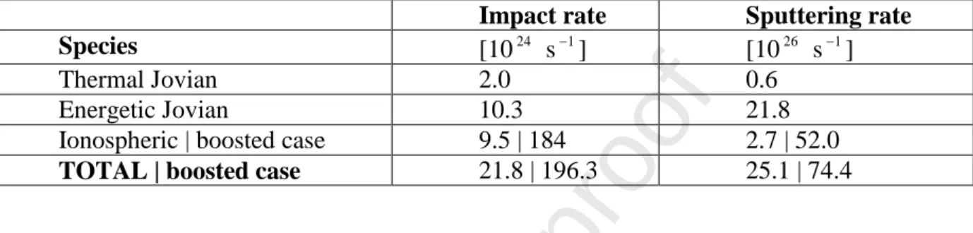
Table 4: Impact rates of different ion populations: thermal Jovian, energetic Jovian, ionospheric with the default exospheric model (last column, left) and a boosted case (
2 10
O
n and a regional increased electron-impact ionization frequency (4), as justified by Carnielli et al. (2019) (last column, right).
Impact rate Sputtering rate
Species [1024 s1] [1026 s1]
Thermal Jovian 2.0 0.6
Energetic Jovian 10.3 21.8
Ionospheric | boosted case 9.5 | 184 2.7 | 52.0
TOTAL | boosted case 21.8 | 196.3 25.1 | 74.4
Table 4 summarizes the impact and sputtering rates contribution from each ion population. For ionospheric ions, the table shows also values for a “boosted” case. These derive from a set of simulations in which the density of O2 from the model of Leblanc et al. (2017) has been multiplied by 10 everywhere and the ionization frequency from electron-impact has been multiplied by 4 in the polar regions in the anti-Jovian hemisphere. Such simulations are discussed in a companion paper, and they are motivated by the underestimated electron number density along the G2 flyby found by the ionospheric model compared with observations (Carnielli et al., 2019). We found that the discrepancy in the electron number density can be removed by adapting the simulation inputs in the way described above, and in the companion paper we discuss in more details the extensive analysis that leads to the choice of this configuration. Here, we simply report how this “boosted case” would modify the total impact and sputtering rates.
In terms of impact rate, ionospheric and energetic Jovian ions provide an approximately equal contribution. However, for the boosted case, the impact rate from ionospheric ions is about 20 times higher. In either case, this population proves to be an important source to consider when studying weathering effects on the moon‟s surface. In terms of sputtering rate, energetic Jovian ions are the main source, with ionospheric ions accounting for approximately 10% of the total rate. However, in the boosted case ionospheric ions become the major source.
Unlike for Jovian ions, sputtering from ionospheric ions is around one order of magnitude more intense in the leading hemisphere than in the trailing one due to the global convection pattern towards the leading hemisphere (see Figure 3). If the true exosphere of Ganymede were like that modeled by Leblanc et al. (2017), then energetic Jovian ions would be the species that contribute the most to the production of exospheric particles: the leading and trailing hemispheres would eject at the same rate (see Table 1), assuming that sublimation is equally efficient in the two hemispheres. However, Hartogh et al. (2013) found that there is more than one order of magnitude difference in the H2O exosphere between the leading and trailing hemispheres. They attributed a possible cause for this difference to the surface composition/temperature, which, they argued, could be different between the two sides. However, if the ionospheric model is run with the “boosted” configuration, then the ionospheric species would be the major source of sputtering
Journal Pre-proof
and their strongly asymmetric sputtering (between leading and trailing hemispheres) would help providing an explanation for the Herschel observations. No further conclusions can be drawn due to the lack of in situ data, but the strong asymmetry observed by Herschel favours the possibility of an asymmetry for the ejection process, which in the ionospheric model occurs only if the exosphere is boosted.
Including all ionospheric and Jovian species, the total sputtering rate on Ganymede‟s surface amounts to 2.5 10 27 s1 in the “non-boosted case”, and to 7.4 10 27 s 1 in the “boosted” case. These rates include the ejection of all neutral species, including those formed only indirectly following radiolysis, such as O2. In their exospheric model, Leblanc et al. (2017) set the ejection rate of H2O to 8.0 10 27 s1
in order to reproduce the observations of Hartogh et al. (2013). This value is higher than the total ejection rate calculated by our model using either configuration in the ionospheric model (the boosted and non-boosted cases). This discrepancy suggests that the sputtering yields at Ganymede could be higher than what calculated using the formula from Famá et al. (2008) and Johnson et al. (2009). The sputtering yield depends on several parameters associated with the sputtered surface, such as its temperature and composition. However, experiments cannot faithfully replicate the conditions at Ganymede‟s surface, thus the empirical profiles for the sputtering yield used in this work might not be fully applicable. It is also possible that Ganymede‟s exosphere has additional sources deriving from sub-surface activity releasing gas like at Europa (Jia et al., 2018) that were not considered in the exospheric model of Leblanc et al. (2017). In the future, it would be worth exploring the reason for the inconsistency between the ejection rate in the exospheric model and the sputtering rate in the ionospheric model. Finally, the impact and sputtering rates are subject to temporal variation. More precisely, the changes are driven by the changing spatial configuration of Ganymede with respect to the Jovian plasma sheet, which changes the incoming flux distribution of Jovian plasma, and the varying position of Ganymede with respect to Jupiter. The orbital motion causes the shift of the illuminated hemisphere, which changes the location of production of ionospheric ions from photo-ionization, and the surface temperature distribution. Since photo-ionization is a minor process compared to electron-impact ionization (Carnielli et al., 2019), we don‟t expect significant changes to occur as a result of the shift of the illuminated hemisphere. However, the sputtering yield is highly dependent on the surface temperature, so the change of spatial distribution of this parameter will have a greater impact on the global ejection rates. Studying the variation of the impact and ejection rates with varying external conditions is worth conducting, but beyond the scope of this work.
5. Conclusions
In this work, we have assessed surface sputtering at Ganymede by simulating ion precipitation from Jupiter‟s magnetosphere and Ganymede‟s ionosphere. Our simulations rely on the test particle code developed by Carnielli et al. (2019), originally applied to Ganymede‟s ionosphere. For ionospheric ions, our simulations constitute the first quantitative estimate of the contribution on sputtering from these species. We have applied the code to simulate the energetic and thermal components of the Jovian plasma. The code recorded the surface impact rate and impact energy for each ion species simulated; with this information, we have calculated the sputtering rate using the expressions from Famá et al. (2008) and Johnson et al. (2009) and generated 2–D maps for the impact flux, sputtering flux, and average impact energy.
Journal Pre-proof
magnetic field lines are open, and in the equatorial region. The impact flux is higher in the polar regions, while sputtering dominates in the equatorial region as the ions that are able to penetrate the closed magnetic field lines have higher energies, and sputter the surface with higher yields. Overall, the sputtering process is driven by energetic S3 ions and peaks at energies near 100 keV. Ionospheric ions are found to impact mainly in the leading hemisphere because of the plasma convection towards the direction of corotation. The impact flux is higher in the polar regions, but like for Jovian plasma, the sputtering flux is significantly higher in the equatorial region. As a result, the ionospheric sputtering flux peaks at low latitudes in the leading hemisphere. Globally, ionospheric ions provide at least 10% of the contribution to the total sputtering. In the case where the O2 exosphere is 10 times denser and the electron-impact ionization frequency is 4 times higher in the anti-Jovian hemisphere, as argued in a companion paper and presented here as the “boosted” case, ionospheric ions sputter more than Jovian ions. In either case, the ionospheric population proves to be an important source to consider when assessing ion precipitation on the moon‟s surface.
Further work includes studying the variation of ion sputtering by varying the input conditions, such as the configuration of Ganymede with respect to the Jovian plasma sheet, which changes the flux distribution of the incoming Jovian plasma, and the position of the moon with respect to Jupiter, which changes the illuminated hemisphere and the surface temperature distribution.
6. Acknowledgments
Work at Imperial College London was supported by STFC of UK through a postgraduate studentship and under grant ST/N000692/1. FL and RM acknowledge the support by the ANR HELIOSARES (ANR-09-BLAN-0223), ANR MARMITE-CNRS (ANR-13-BS05-0012-02) and by the “Système Solaire” program of the French Space Agency CNES. XJ acknowledges support by NASA‟s Solar System Workings program through grant NNX15AH28G. Authors also warmly acknowledge the support of the IPSL data centre CICLAD for providing access to their computing resources.
References
Carnielli, G., Galand, M., Leblanc, F., Leclercq, L., Modolo, R., Beth, A., Huybrighs, H.L.F., Jia, X., 2019. First 3D test particle model of Ganymede‟s ionosphere. Icarus 330, 42–59. URL: https://ui.adsabs.harvard.edu/abs/2019Icar..330...42C, doi: 10.1016/j.icarus.2019.04.016.
Cooper, J.F., Johnson, R.E., Mauk, B.H., Garrett, H.B., Gehrels, N., 2001. Energetic Ion and Electron Irradiation of the Icy Galilean Satellites. Icarus 149, 133–159. URL: http://adsabs.harvard.edu/abs/2001Icar..149..133C, doi: 10.1006/icar.2000.6498.
Famá, M., Shi, J., Baragiola, R.A., 2008. Sputtering of ice by low-energy ions. Surface Science 602, 156–161. URL: http://adsabs.harvard.edu/abs/2008SurSc.602..156F, doi: 10.1016/j.susc.2007.10.002.
Fatemi, S., Poppe, A.R., Khurana, K.K., Holmström, M., Delory, G.T., 2016. On the formation of Ganymede‟s surface brightness asymmetries: Kinetic simulations of Ganymede‟s magnetosphere. Geophysical Research Letters 43, 4745–4754. URL:
Journal Pre-proof
Frank, L.A., Paterson, W.R., Ackerson, K.L., Bolton, S.J., 1997. Outflow of hydrogen ions from Ganymede. Geophysical Research Letters 24, 2151. URL: http://adsabs.harvard.edu/abs/1997GeoRL..24.2151F, doi: 10.1029/97GL01744.
Galli, A., Vorburger, A., Wurz, P., Tulej, M., 2017. Sputtering of water ice films: A re-assessment with singly and doubly charged oxygen and argon ions, molecular oxygen, and electrons. Icarus 291, 36–45. URL: https://ui.adsabs.harvard.edu/abs/2017Icar..291...36G, doi: 10.1016/j.icarus.2017.03.018.
Hartogh, P., Bockelee-Morvan, D., Rezac, L., Moreno, R., Lellouch, E., Rengel, M., Jarchow, C., de Val-Borro, M., Crovisier, J., Biver, N., 2013. Detection and
Characterisation of Ganymede‟s and Callisto‟s Water Atmospheres. Presented at the international symposium “The universe explored by Herschel” 15-18 October 2013, ESTEC, Netherlands URL: http://herschel.esac.esa.int/TheUniverseExploredByHerschel/presentation
s/13a-1720_HartoghP.pdf.
Ip, W.H., Williams, D.J., McEntire, R.W., Mauk, B., 1997. Energetic ion sputtering effects at Ganymede. Geophysical Research Letters 24, 2631. URL:
http://adsabs.harvard.edu/abs/1997GeoRL..24.2631I, doi: 10.1029/97GL02814.
Jia, X., Kivelson, M.G., Khurana, K.K., Kurth, W.S., 2018. Evidence of a plume on Europa from Galileo magnetic and plasma wave signatures. Nature Astronomy 2, 459–464. URL: http://adsabs.harvard.edu/abs/2018NatAs...2..459J, doi:
10.1038/s41550-018-0450-z.
Jia, X., Walker, R.J., Kivelson, M.G., Khurana, K.K., Linker, J.A., 2009. Properties of Ganymede‟s magnetosphere inferred from improved three-dimensional MHD simulations. Journal of Geophysical Research (Space Physics) 114, A09209. URL: http://adsabs.harvard.edu/abs/2009JGRA..114.9209J, doi: 10.1029/2009JA014375.
Johnson, R.E., 1990. Energetic Charged-Particle Interactions with Atmospheres and Surfaces. Springer-Verlag Berlin Heidelberg. doi: 10.1007/978-3-642-48375-2.
Johnson, R.E., Burger, M.H., Cassidy, T.A., Leblanc, F., Marconi, M., Smyth, W.H., 2009. Composition and Detection of Europa‟s Sputter-induced Atmosphere. p. 507. URL: http://www.people.virginia.edu/ ~rej/papers09/Johnson4005.pdf.
Johnson, R.E., Carlson, R.W., Cooper, J.F., Paranicas, C., Moore, M.H., Wong, M.C., 2004. Radiation Effects on the Surfaces of the Galilean Satellites. pp. 485–512. URL: http://lasp.colorado.edu/~espoclass/homework/5830_2008_homework/Ch20.pdf.
Keppler, E., Krupp, N., 1996. The charge state of helium in the Jovian magnetosphere: a possible method to determine it. Planetary and Space Science 44, 71–75. URL:
http://adsabs.harvard.edu/abs/1996P%26SS...44...71K doi: 10.1016/0032-0633(95)00076-3. Kivelson, M.G., Bagenal, F., Kurth, W.S., Neubauer, F.M., Paranicas, C., Saur, J., 2004. Magnetospheric interactions with satellites. pp. 513–536. URL:
http://www.igpp.ucla.edu/public/mkivelso/Publications/Ch21.pdf.
Lanzerotti, L.J., Brown, W.L., Poate, J.M., Augustyniak, W.M., 1978. On the contribution of water products from Galilean satellites to the Jovian magnetosphere. Geophysical Research Letters 5, 155–158. URL: http://adsabs.harvard.edu/abs/1978GeoRL...5..155L, doi: 10.1029/GL005i002p00155.
Leblanc, F., Oza, A.V., Leclercq, L., Schmidt, C., Cassidy, T., Modolo, R., Chaufray, J.Y., Johnson, R.E., 2017. On the orbital variability of Ganymede‟s atmosphere. Icarus 293, 185–198. URL: http://adsabs.harvard.edu/abs/2017Icar..293..185L, doi: 10.1016/j.icarus.2017.04.025.
Journal Pre-proof
Mauk, B.H., Mitchell, D.G., McEntire, R.W., Paranicas, C.P., Roelof, E.C.,
Williams, D.J., Krimigis, S.M., Lagg, A., 2004. Energetic ion characteristics and neutral gas interactions in Jupiter‟s magnetosphere. Journal of Geophysical Research (Space Physics) 109, A09S12. URL: http://adsabs.harvard.edu/abs/2004JGRA..109.9S12M, doi:
10.1029/2003JA010270.
Neubauer, F.M., 1998. The sub-Alfvénic interaction of the Galilean satellites with the Jovian magnetosphere. Journal of Geophysical Research 103, 19843–19866. URL: http://adsabs.harvard.edu/abs/1998JGR...10319843N, doi: 10.1029/97JE03370.
Paranicas, C., Paterson, W.R., Cheng, A.F., Mauk, B.H., McEntire, R.W., Frank, L.A., Williams, D.J., 1999. Energetic particle observations near Ganymede. Journal of Geophysical Research 104, 17459–17470. URL:
http://adsabs.harvard.edu/abs/1999JGR...10417459P, doi: 10.1029/1999JA900199. Pilcher, C.B., 1976. Stability of water on the Galilean satellites, in: Bowen, S.L., Wright, E. (Eds.), Water in Planetary Regoliths, p. 65. URL:
http://adsabs.harvard.edu/abs/1976wpr..conf...65P.
Plainaki, C., Milillo, A., Massetti, S., Mura, A., Jia, X., Orsini, S., Mangano, V., De Angelis, E., Rispoli, R., 2015. The H2O and O2 exospheres of Ganymede: The result of a complex interaction between the jovian magnetospheric ions and the icy moon. Icarus 245, 306–319. URL: http://adsabs.harvard.edu/abs/2015Icar..245..306P, doi:
10.1016/j.icarus.2014.09.018.
Poppe, A.R., Fatemi, S., Khurana, K.K., 2018. Thermal and Energetic Ion Dynamics in Ganymede‟s Magnetosphere. Journal of Geophysical Research (Space Physics) 123, 4614– 4637. URL: http://adsabs.harvard.edu/abs/2018JGRA..123.4614P, doi:
10.1029/2018JA025312.
Qin, H., Zhang, S., Xiao, J., Liu, J., Sun, Y., Tang, W.M., 2013. Why is Boris algorithm so good? Physics of Plasmas 20, 084503. URL:
http://adsabs.harvard.edu/abs/2013PhPl...20h4503Q, doi: 10.1063/1.4818428.
Shi, M., Baragiola, R.A., Grosjean, D.E., Johnson, R.E., Jurac, S., Schou, J., 1995. Sputtering of water ice surfaces and the production of extended neutral atmospheres. Journal of Geophysical Research 100, 26387–26396. URL:
http://adsabs.harvard.edu/abs/1995JGR...10026387S, doi: 10.1029/95JE03099.
Teolis, B.D., Plainaki, C., Cassidy, T.A., Raut, U., 2017. Water Ice Radiolytic O2, H2, and H2O2 Yields for Any Projectile Species, Energy, or Temperature: A Model for Icy Astrophysical Bodies. Journal of Geophysical Research (Planets) 122, 1996–2012. URL: https://ui.adsabs.harvard.edu/abs/2017JGRE..122.1996T, doi: 10.1002/2017JE005285.
Journal Pre-proof
Highlights
Sputtering of Ganymede’s ionospheric ions provides a significant contribution to the moon’s exosphere
Ionospheric O2+ is the major contributor for surface sputtering
Ionospheric sputtering occurs mainly in the leading hemisphere at low latitudes
Ionospheric sputtering could explain the asymmetry in the H2O density observed by