HAL Id: hal-01088662
https://hal.archives-ouvertes.fr/hal-01088662
Submitted on 8 Nov 2017
HAL is a multi-disciplinary open access
archive for the deposit and dissemination of
sci-entific research documents, whether they are
pub-lished or not. The documents may come from
teaching and research institutions in France or
abroad, or from public or private research centers.
L’archive ouverte pluridisciplinaire HAL, est
destinée au dépôt et à la diffusion de documents
scientifiques de niveau recherche, publiés ou non,
émanant des établissements d’enseignement et de
recherche français ou étrangers, des laboratoires
publics ou privés.
N. Romanelli, Ronan Modolo, E. Dubinin, Jean-Jacques Berthelier, C.
Bertucci, J. E. Wahlund, François Leblanc, Patrick Canu, Niklas Jt Edberg,
H. Waite, et al.
To cite this version:
N. Romanelli, Ronan Modolo, E. Dubinin, Jean-Jacques Berthelier, C. Bertucci, et al.. Outflow and
plasma acceleration in Titan’s induced magnetotail: Evidence of magnetic tension forces. Journal of
Geophysical Research Space Physics, American Geophysical Union/Wiley, 2014, 119 (12),
pp.9992-10005. �10.1002/2014JA020391�. �hal-01088662�
RESEARCH ARTICLE
10.1002/2014JA020391 Key Points:
• Ionospheric plasma is observed in Titan’s wake
• The plasma acceleration is analyzed through Walen tests
• This acceleration can be understood in terms of magnetic tension forces
Correspondence to:
N. Romanelli, [email protected]
Citation:
Romanelli, N., et al. (2014), Outflow and plasma acceleration in Titan’s induced magnetotail: Evidence of magnetic ten-sion forces, J. Geophys. Res.
Space Physics, 119, 9992–10,005,
doi:10.1002/2014JA020391.
Received 18 JUL 2014 Accepted 18 NOV 2014
Accepted article online 26 NOV 2014 Published online 19 DEC 2014
Outflow and plasma acceleration in Titan’s induced
magnetotail: Evidence of magnetic tension forces
N. Romanelli1, R. Modolo2, E. Dubinin3, J.-J. Berthelier2, C. Bertucci1, J. E. Wahlund4, F. Leblanc2,
P. Canu5, N. J. T. Edberg4, H. Waite6, W. S. Kurth7, D. Gurnett7, A. Coates8, and M. Dougherty9 1Institute for Astronomy and Space Physics, Ciudad Universitaria, Buenos Aires, Argentina,2LATMOS, UVSQ Guyancourt, France,3Max Planck Institute, MPS, Lindau, Germany,4Swedish Institute of Space Physics, Uppsala, Sweden,5Laboratoire de Physique des Plasmas, Ecole Polytechnique, Palaiseau, France,6Southwest Research Institute, San Antonio, Texas, USA, 7Department of Physics and Astronomy, University of Iowa, Iowa, USA,8MSSL, University College London, London, UK, 9Space and Atmospheric Physics Group, The Blackett Laboratory, Imperial College London, London, UK
Abstract
Cassini plasma wave and particle observations are combined with magnetometer measurements to study Titan’s induced magnetic tail. In this study, we report and analyze the plasma acceleration in Titan’s induced magnetotail observed in flybys T17, T19, and T40. Radio and Plasma Wave Science observations show regions of cold plasma with electron densities between 0.1 and a few tens of electrons per cubic centimeter. The Cassini Plasma Spectrometer (CAPS)-ion mass spectrometer (IMS) measurements suggest that ionospheric plasma in this region is composed of ions with masses ranging from 15 to 17 amu and from 28 to 31 amu. From these measurements, we determine the bulk velocity of the plasma and the Alfvén velocity in Titan’s tail region. Finally, a Walén test of such measurements suggest that the progressive acceleration of the ionospheric plasma shown by CAPS can be interpreted in terms of magnetic tension forces.1. Introduction
Several observations in Titan’s tail have shown that ionospheric plasma populations are being transported downstream from the moon as a result of the interaction with the Kronian plasma. Gurnett et al. [1982] stud-ied the structure of Titan’s wake from Voyager 1 measurements. Based on pressure balance considerations, they suggested that the plasma observed in the neutral sheet was originated at the ionosphere of the moon.
Gurnett et al. [1982] also estimated that the total loss rate of ionospheric ions is about 1.2 × 1024ions s−1.
More recently, Wahlund et al. [2005] analyzed the cold plasma environment around Titan and provided the first ionospheric outflow determination derived from Cassini observations: this value was estimated to be 1025ions s−1. Coates et al. [2007] and Szego et al. [2007] reported on the presence of ionospheric plasma at
several Titan radii in the tail region during Cassini flyby T9 and Modolo et al. [2007a, 2007b] estimated an associated outflow ranging between 2 and 7 ×1025ions s−1. Sittler et al. [2010] complemented these
stud-ies and estimated that the ionospheric flux flowing away from Titan (for the so-called Event 1) is ∼ 7 × 10⁶
ion cm−2s−1. Edberg et al. [2011] analyzed Radio and Plasma Wave Science (RPWS)-Langmuir Probe
observa-tions during consecutive and similar Cassini Titan flybys T55-T59. They found a region with high (1–8 cm−3)
plasma densities in the tail/nightside of the moon at locations progressively farther downtail from pass to pass. They described their results as a steady structure of ionospheric plasma escaping from Titan. Edberg
et al. [2011] suggested three possible acceleration mechanisms which could have contributed to this
iono-spheric outflow: the ambipolar electric field (similar to Earth’s polar wind), the magnetic moment pumping, and dispersive Alfvén waves. However, they could not conclude which mechanism is responsible for the observed acceleration. Analyses of Cassini Plasma Spectrometer (CAPS) electron and ion observations at Titan’s distant tail have also been investigated by Coates et al. [2012]. They studied crossings of Titan’s tail during flybys T9, T63, and T75 and identified the presence of ionospheric plasma in that region. Some of the electron spectra indicate a direct magnetic connection to Titan’s dayside ionosphere, while ion obser-vations reveal heavy (m/q ∼16 and 28) as well as light (m/q = 1–2) ion populations streaming down the tail. They suggested that the ambipolar electric field may be the driver of the ion escape. They estimated a total plasma loss rate from Titan of the order of ∼ 1024ions s−1for the three flybys. In addition to the previous
studies, Cui et al. [2010] derived a total ion loss rate from Titan of 1.7 × 1025ions s−1based on
composition for T40 flyby close to Titan can be found in Westlake et al. [2012]. Based on Cassini Ion and Neutral Mass Spectrometer (INMS) observations obtained at altitudes ranging between 2225 km and 3034 km, the authors found significant densities of CH+
5, HCNH+, and C2H+5. Taking into account this
composi-tion as well as the ion velocities, they suggested that these ions must have been created below the exobase and transported to the detection altitude by a combination of thermal pressure and magnetic forces. They also pointed out that this outward flow might link the gravitationally bound ionosphere with the more distant wake.
In the present study we investigate the role of the magnetic tension forces in the acceleration of ionospheric plasma in the wake of Titan. We will do so by applying the formalism of magnetohydrodynamics (MHD) to interpret Cassini’s data in Titan’s tail. These forces are expected to be important near Titan’s plasma sheet as well as in regions where Alfvénic structures are present. In these structures, the components of the plasma velocity tangential to those layers change in response to the J × Bnforce (Bn= B⋅ ̂n, where ̂n is the normal to the discontinuity plane). As is stated in Paschmann and Sonnerup [2008], a plasma flowing across such structures satisfies the Walén relation:
Δv = ±ΔvA (1)
where Δv and ΔvAare the variations in the plasma and Alfvén velocities, respectively.
As is also shown in Appendix A, in the case of an incompressible fluid an exact solution to the ideal MHD equations can be found where the changes in the bulk velocity of the plasma due to magnetic tension forces satisfy the Walén relation. This relation has a much simpler formulation in the deHoffmann-Teller frame (HT) [Khrabrov and Sonnerup, 1998], a reference frame where the electric field in the plasma is zero. In this reference frame, the Walén relation can be written as (see Appendix A or Paschmann and Sonnerup [2008])
v′= ±v
A (2)
where v′and v
Aare the plasma bulk velocity and the Alfvén velocity in the HT frame, respectively. Therefore, according to the derivation of equation (2), the J × B force accelerates the plasma flow which, seen from the HT reference frame, is characterized by an Alfvénic bulk velocity whose direction is parallel or antiparallel to the local magnetic field.
The HT analysis/Walén test [Khrabrov and Sonnerup, 1998] is usually applied to study plasma acceleration events in the presence of discontinuities or current layers in order to establish if the magnetic tension forces arising in these layers can be accountable for the changes in the kinetic energy of the plasma. The Walén test consists of finding an approximate HT reference frame and then plotting the estimated plasma bulk velocity components, after transformation into the HT frame, against the corresponding components of the calculated local Alfvén velocities. In the present study we analyze Cassini plasma observations obtained during three flybys. We consider flybys T17, T19, and T40 since in these cases Cassini’s trajectory explored Titan’s induced magnetotail and was allowed to characterize Titan’s plasma outflow. We also verify that the MHD formalism can be applied for the considered data set before testing the Walén relation. Additionally, we also perform a minimum variance analysis (MVA) of the magnetic field measurements to determine if they display signatures of the existence of current layers compatible with tension forces [Sonnerup and
Scheible, 1998].
This study is structured as follows: A brief description of each used instrument is presented in section 2. Analysis of ion fluxes, angular distribution, mass composition, and energy spectra are presented for the T40 flyby in section 3. This information allows the estimation of the plasma velocity in Titan’s wake, which combined with electron number density and magnetic field observations yields the local Alfvén speed and the ionospheric fluxes flowing away from Titan. The deHoffmann-Teller analysis, the Walén test, and the MVA results are also presented in section 3. In section 4 we summarize and discuss our results for the three considered flybys.
2. Instrument Description
Magnetic field observations are derived from the Cassini Magnetic field experiment [Dougherty et al., 2004], ion composition and plasma flow information are obtained from CAPS [Young et al., 2004], and elec-tron number density and spacecraft potential are calculated from RPWS/LP [Gurnett et al., 2004]. In this section we present a brief description of each of these instruments.
2.1. Magnetometer (MAG)
The Cassini Magnetic field experiment consists of a Vector Helium Magnetometer (VHM) and a Fluxgate Magnetometer (FGM) capable of measuring the ambient magnetic field over a wide range: ± 256 nT and ± 65655 nT, respectively. The vector measurements provided by the VHM and the FGM have a resolution of 2 Hz and 32 Hz, respectively [Dougherty et al., 2004]. In this study we use 1 s averaged FGM vector magnetic field measurements.
2.2. CAPS-Electron Spectrometer Sensor
The Cassini Particle Spectrometer-Electron Spectrometer Sensor (CAPS-ELS) measures electrons in the energy range of 0.6 eV–28 keV with an energy resolution ΔE∕E = 0.17 and an angular resolution of 20◦[Young et al., 2004]. In this study we have used electron density estimates derived from the moment calculations [Lewis et al., 2008].
2.3. CAPS-Ion Mass Spectrometer
CAPS-ion mass spectrometer (IMS) samples ions in eight angular sectors (anodes) with each sector having an instantaneous field of view (FOV) of 8◦× 20◦. This instrument takes singles data (SNG), start signals gen-erated by the detection of electrons libgen-erated from the carbon foil [Thomsen et al., 2010], corresponding to energy-per-charge spectra ranging from 1 eV to 50 keV with a spectral resolution of 17%. The 63 step energy sweeps, and the 64th step (the fly-back bin) take 4.0 s to acquire the data and are formatted into eight energy sweeps per instrument’s internal data acquisition cycle. This cycle, referred to as the A cycle, lasts 32.0 s. The CAPS-IMS sensors are mounted on a rotating platform capable of actuating the CAPS instrument by ∼180◦around an axis parallel to the spacecraft Z axis in about 3 min. The time-of-flight (TOF) analyzer is used to infer detailed compositional analysis in a so-called B cycle. The B cycle lasts eight A cycle, i.e., 256 s. During the B cycle, the eight angular sectors are summed together and the 64 steps are collapsed to 32 energy steps. More detailed information of CAPS-IMS are presented in Young et al. [2004], Hartle et al. [2006],
Sittler et al. [2010], and Wilson et al. [2012]. These observations are used to characterize the ion population
and provide key information about the plasma flow direction, its composition, and the relative abundance of its constitutive ion species.
2.4. RPWS
The Radio and Plasma Wave Science (RPWS) investigation consists of three orthogonal electric field anten-nas, three orthogonal search coil magnetic antenanten-nas, and a Langmuir probe (LP) [Gurnett et al., 2004]. In the present study, we use the LP and the High- and Medium-Frequency Receiver observations since they provide two independent estimates for the electron number density [e.g., Edberg et al., 2010]. RPWS observations, in conjunction with the CAPS-ELS measurements, provide estimates for the electron number density at different regions around Titan. Even though the CAPS-ELS moment calculation may underesti-mate the electron number density at regions where Cassini is negatively charged (since it cannot observe a fraction of low-energy electrons), it is a well-designed instrument for regions of hot plasmas such as that of Titan’s surrounding environment [Lewis et al., 2008]. In contrast, the electrostatic wave emissions are observed only at locations where the electron density is≳ 0.1 cm−3. Therefore, the RPWS instrument
pro-vides reliable measurements in regions very close to Titan, which mainly contain cold plasma. The two data sets are complementary and provide a complete characterization of the electron density in Titan’s vicinity. The next section presents Cassini observations followed by a step by step description of the analysis under-taken for this investigation. The detailed analyses are presented for the T40 flyby, but a similar study has been performed for T17 and T19 flybys.
3. CAPS/RPWS/MAG Analysis: The T40 Case
3.1. Observations
Cassini’s Titan flyby T40 took place on 5 January 2008 with the closest approach at an altitude of 949 km (at 21:26:24 UTC). Saturn local time was 11.3 h, as a result the angle between Titan’s nightside and Titan’s nominal corotation wake is close to 90◦. Figure 1 shows CAPS-IMS, CAPS-ELS, RPWS, and MAG observa-tions for this flyby in the time interval 20:30–22:30 UTC. Figure 1 (top) shows the eight-anode average of the CAPS-IMS singles observations. Figure 1 (middle) displays the electron number density derived by CAPS-ELS moment calculation (blue marks), LP analysis (red marks), and deduced from the upper hybrid frequency (green marks). Electron number density deduced from ELS in the time interval 21:08 to 21:45 are not shown.
Figure 1. CAPS, RPWS, and MAG observations for T40 flyby (2008, day of year 5). (top) The eight anodes average of the CAPS-IMS observations. (middle) The electron number density derived by CAPS-ELS moment calculation (blue marks), LP analysis (red marks), and deduced from wave observations (green marks). (bottom) The magnetic field components measured by MAG:BxTIIS(blue curve),ByTIIS(green curve),BzTIIS(red curve), and the magnetic field intensityBTIIS
(black curve).
Figure 1 (bottom) presents the magnetic field components measured by MAG in Titan Ionospheric Interac-tion coordinates (TIIS). In this Titan-centered coordinate system the XTIISaxis points in the direction of ideal
corotation, the YTIISaxis points toward Saturn, and the ZTIISaxis completes the right-handed system. The blue, green, and red curves show the BxTIIS, ByTIIS, and BzTIISmagnetic field components, respectively, while the black curve displays the magnetic field intensity BTIIS.
From all data sets shown in Figure 1 it can be noted that Cassini is located in Saturn’s magnetosphere between 20:30 and 20:50 UTC. This plasma region is characterized by an electron number density ranging between 0.01 and 0.1 cm−3. At about 20:50 UTC, Cassini enters Titan’s induced magnetosphere and the
elec-tron density increases, while the spacecraft approaches Titan’s ionosphere. Density estimates derived from LP analysis, plasma wave, or moment calculation from particle analyzer show similar values. Between 20:53 and 21:15 UTC, the observed energy of the ion plasma smoothly decreases from ∼ 50 eV to ∼5 eV. At the same time, MAG measurements show that Cassini is in the away (BxTIIS > 0) lobe of Titan’s magnetotail.
The entry into the induced magnetosphere can be noticed from the increment in BxTIIS, while the other two components decrease. Note that in the case of ideal magnetospheric plasma corotation, the direction of the XTIISmagnetic field component is the same as the direction of the ideal external plasma flow. As can be
seen, Cassini remains in the away lobe of Titan’s magnetotail until the reversal of the BxTIISmagnetic field
component at about 21:21 UTC. Finally, Cassini leaves Titan’s induced magnetosphere in the time frame 21:47–21:50 UTC. In this study we test if the observed changes in the kinetic energy of the plasma (Figure 1, top) can be associated with magnetic tension forces present during the same time intervals.
Sections 3.2, 3.3, and 3.4 describe the analyses performed on CAPS/RPWS/MAG measurements in order to estimate the bulk velocity of the plasma and the local Alfvén velocity in Titan’s induced tail. The analyses are carried out in the Kronocentric Solar Orbital (KSO) coordinate system. This coordinate system is centered at Saturn with the XKSOaxis pointing toward the Sun, the ZKSObeing perpendicular to the plane of Saturn’s orbital motion and pointing north of the ecliptic and YKSOcompleting the right-handed system.
Figure 2. (a) Normalized single ion fluxes (color coded) measured by CAPS from 21:09 to 21:12 hs as a function of𝛿and𝜃. The mark also indicates the position associated with the flow direction:𝛿 = 35◦and𝜃 = −130◦. (b) Energy spectra of the single ion fluxes observed by each of the eight anodes of CAPS at 21:10:30 hs. The red curve identifies the anode number 5 where the ion flux takes its highest value.
3.2. Plasma Flow Direction
The determination of the flow direction is computed from the CAPS singles (SNG) data and makes use of the instantaneous FOV of CAPS-IMS, the actuator position, and the spacecraft orientation. There is no mass dis-crimination in the SNG data, but elevation and azimuthal information allows us to reconstruct the angular distribution. During one actuator scan the instrument is able to cover a wider region which, due to its geo-metrical capabilities, is limited to about 2𝜋 steradian (for a fixed spacecraft orientation). The sky map seen by the instrument is a sphere where a given point can be defined with two spherical coordinates,𝛿 and 𝜃. The angle between the ZKSO= 0 plane and the position r is𝛿; 𝛿 can be seen as a latitude which ranges from
−90◦to +90◦. The longitudinal angle𝜃 is contained in the XKSO− YKSOplane and takes values between
−180◦and +180◦, where𝜃 = 0◦corresponds to the direction of the XKSOaxis. Taking into account the
intrinsic angular acceptance of the analyzer, the actuator motion and the spacecraft orientation, we derive the spatial coverage of each anode at each acquisition time by means of SNG data. By integrating over all energy bins we can estimate the total number of counts received for each anode at each accumulation time. Plotting this information in a𝛿-𝜃 map for a short time interval (basically one actuator scan) allows the recon-struction of the angular distribution of the plasma in the spacecraft frame, in the KSO coordinate system. The flow direction is determined when the core of the distribution function is observed and identified with specific values of𝛿 and 𝜃. The uncertainties in the spherical coordinates are Δ𝛿 = 20◦and Δ𝜃 = 20◦. Figure 2a displays the single ion fluxes measured by CAPS from 21:09 to 21:12 UTC (during flyby T40) as a function of𝛿 and 𝜃 and also points out the position associated with the flow direction. In this case, the angles are𝛿 = 35◦and𝜃 = −130◦. The plasma flow direction has been determined for different time inter-vals when the incoming plasma was in the FOV of the instrument. These results are summarized in Table 1, columns 3 and 4.
3.3. Plasma Flow Speed
Determining the plasma speed requires information such as the plasma composition, the observed energy, and the spacecraft potential. Unfortunately, TOF measurements do not always allow a mass determination since the ion flux might not be intense enough. The knowledge of the ion composition is then limited to only a few time intervals. However, assuming that the different ion species are traveling at the same velocity
v, it is possible to use SNG data in a complementary way. In this case, different energy spectra peaks reflect the different ion composition of the plasma under study. Most of the time, two energy peaks are observed and correspond to two ion mass groups. TOF data analyses, when sufficient counts allow a good mass deter-mination, are used to identify more accurately the ion masses. In these cases, ratios of the main ion mass groups deduced from the TOF analysis are consistent with the energy ratio of the SNG spectra. This result suggests that the different ion populations are traveling with the same speed. As a consequence, the MHD
Ta b le 1 . CAPS Analy sis fo r F lyb y T17, T19, and T 40: V e locit y Det e rmination a Tb Te 𝛿𝜃 Ts AE ′ 1 F1 E ′ 2 F2 Usc E1 ∕ E2 C1 C2 m1 m2 < m > (UT C ) (UT C ) ( ◦)( ◦) (UT C ) (eV ) (cm − 2sr − 1s − 1)( e V )( cm − 2sr − 1s − 1) (eV ) (amu) (amu) (amu) Fl yb y T17 19:56:30 19:59:00 − 28 60 19:57:40 5 11.32 1.45 × 10 7 6.72 1.20 × 10 7 − 1.15 1.82 0.55 0.45 31 16 24.22 20:00:30 20:02:30 − 28 52 20:01:30 5 13.46 8.84 × 10 6 6.73 2.90 × 10 7 − 1.06 2.19 0.23 0.77 31 16 19.50 20:02:30 20:04:10 − 28 52 20:03:20 5 8.00 2.53 × 10 7 4.76 2.40 × 10 7 − 1.29 1.93 0.51 0.49 31 16 23.70 20:04:20 20:05:50 − 28 52 20:05:00 5 6.73 2.10 × 10 7 4.00 1.76 × 10 7 − 1.11 1.94 0.54 0.46 31 16 24.16 20:06:10 20:07:30 − 28 52 20:06:45 5 6.73 6.64 × 10 6 –– − 1.29 – 1.00 0.00 31 – 31.00 Fl yb y T19 17:07 17:10 − 20 65 17:07:40 6 38.07 6.04 × 10 6 22.63 1.25 × 10 6 − 0.26 1.69 0.83 0.17 28 17 26.11 17:10 17:13 − 35 65 17:12:40 7 22.63 1.42 × 10 7 13.46 8.59 × 10 6 − 0.63 1.71 0.62 0.38 28 17 23.85 17:13 17:15 − 35 65 17:14:10 7 13.46 1.26 × 10 7 8.00 9.27 × 10 6 − 0.85 1.76 0.58 0.42 28 17 23.34 17:15 17:17 − 35 65 17:15:55 7 13.46 5.93 × 10 6 8.00 1.64 × 10 7 − 1.08 1.79 0.27 0.73 28 17 19.92 17:17 17:18 − 35 65 17:17:25 7 9.51 9.16 × 10 6 6.72 1.00 × 10 7 − 0.95 1.48 0.48 0.52 28 17 22.26 17:18 17:20 − 35 65 17:19:20 7 8.02 2.57 × 10 7 4.76 1.98 × 10 7 − 0.75 1.81 0.56 0.44 28 17 23.21 Fl yb y T40 20:59 21:03 45 − 55 21:00:30 4 32.00 2.46 × 10 6 22.63 2.71 × 10 6 0.31 1.41 0.48 0.52 28 17 22.23 21:03 21:06 40 − 75 21:04:00 4 22.63 2.73 × 10 6 13.46 1.98 × 10 6 − 0.21 1.69 0.58 0.42 28 17 23.38 21:06 21:09 25 − 140 21:07:30 4 22.63 1.06 × 10 7 13.46 3.09 × 10 6 − 0.40 1.70 0.77 0.23 28 17 25.52 21:09 21:12 35 − 130 21:10:30 5 16.00 2.08 × 10 7 9.51 7.57 × 10 6 − 0.37 1.71 0.73 0.27 28 17 25.06 aC o lumns 1 a nd 2 sho w the beg inning ( Tb ) a nd ending ( Te ) times of the selec te d int er val .C o lumns 3 a nd 4 d ispla y the angles 𝛿 and 𝜃 associat e d to the flo w d ir ec tion. C olumns 5 a nd 6 spec-ify the time in which the ener gy spec tra w as analyz ed ( Ts ) a nd the a node ( A ) w ith the highest fl ux. C olumns 7 a nd 8 sho w the ener gy peak E ′(without1 the USC co rr ec tion) a nd the cor re sponding flux F1 fo r the species o f m ass m1 , w hile co lumns 9 a nd 10 sho w the same p ro per ties for the species of mass m2 . C olumns 11–14 displa y the values o f USC , E1 ∕ E2 , a nd the p ro por tions o f e ach species in the to tal m ass fl ux ( C1 and C2 ). C o lumns 15–17 sho w the m ass o f e ach species m1 , m2 ,a nd the a v e rage mass value < m > of the fl o w .
E/q ST TOF channel counts (log10) 0 50 100 150 200 250 10 100 1000 10000 0 0.5 1 1.5 50 100 150 200 250 300 350 400 450 500 10−1 100 101 (1) (3) (2) (4) ST TOF bin Counts 50 100 150 200 250 300 350 400 450 500 0 20 40 60 80 100 ST TOF bin Normalized counts CH3+ CH4+ CH5+ HCNH+ C2H5+ TOF data TOF simu
Figure 3. (left) Number of counts on the ST detector, color coded with a logarithmic scale, plotted as a function of the energy per charge (E/q(eV)) and the TOF channels. (top right) Simulated signatures as a function of the TOF channel for the following species: CH+3, CH+4, CH+5, HCNH+, and C
2H+5. (bottom right) Number of counts as a function of the TOF channel derived from TOF data (red curve) and the TOF simulated result (black curve).
formalism can be applied in this environment. The plasma speed is v =√2 Es∕ms, where Esis the energy of the peak corresponding to the population of mass ms(after corrections involving the spacecraft potential
USC). As a result, the ratio between the energy of these two peaks is equal to the ratio between the masses
of the corresponding populations (E1,2= 1∕2 m1,2v2, E1∕E2= m1∕m2). This ratio remains relatively constant
for the different ion spectral signatures of the flyby, suggesting that the plasma composition does not vary significantly during the studied time intervals.
The velocity vector VKSOis determined as
VKSO= −v (cos(𝜃) cos(𝛿) ̂XKSO+ sin(𝜃) cos(𝛿) ̂YKSO+ sin(𝛿) ̂ZKSO) (3)
In this study we consider an uncertainty in the energy values of ΔE = 0.2 E. The minus sign in equation (3) reflects that the plasma flow direction is antiparallel to the normal of the spherical map seen by CAPS. The speed of the plasma flow has been calculated for the same time intervals where the plasma flow direction has been derived (previous subsection). Information on the derived energy and mass of each population is summarized in Table 1.
Next, we show an example based on TOF and SNG data for one event during flyby T40. Figure 3 (left) dis-plays the best TOF measurements, in terms of counts, in the considered tail region. The plot shows the number of counts measured by the Straight Through (ST) detector at about 21:16 UTC in the function of energy per charge (E/q (eV)) and time-of-flight channels. The ion energy ranges from 1 to approximately 10 eV, and several TOF channels exhibit significant counts. The determination of the corresponding mass has been examined with a simulation model developed by Nelson and Berthelier (internal report). This simula-tion model mimics the instrumental response to various ion (molecular and atomic) mass, and energy and has been validated by comparing simulation results with CAPS spare model calibration tests. The expected signature on the ST for a 10–50 eV CH+
5ion beam is presented in green in Figure 3 (top right). The largest
peak at TOF bin 150 corresponds to a start time generated by an electron impact on the ST microchannel plate (MCP) and a stop time due to a neutral carbon impact on the ST MCP. Additionally, for CH+
5, the peak at
TOF bin 100 corresponds to a start and stop time induced by an electron and a negatively charged carbon, while the broader contribution of the signature, from TOF bin 30 to 60, is due to a start time of an elec-tron impact and a stop time of a secondary elecelec-tron created after a neutral hydrogen or carbon impact on the high voltage rings. Each ion species has its own TOF signature, and by testing possible combinations of species one can construct an ion-summed ST signature, which can be compared to the ST observations. The simulation analysis suggests that these peaks are due to the existence of CH+
3, CH + 4, CH + 5, HCNH +, and
C2H+5. Water group ions show O
100 eV). The absence of significant counts at these TOF bins allows excluding water group ions from the plasma composition. Figure 3 (bottom right) shows the number of counts derived from TOF data (red curve) and the TOF simulated result (black curve) when these ion species are considered. We find a good agree-ment between these two curves: the peak marked as (1) is mainly related to the presence of C2H+
5, while the
peak marked as (3) is associated with the existence of CH+
5, HCNH+, and C2H+5. The peaks corresponding to
the heavier ions, marked as (2) and (4) are related to the CH+
3, CH+4, CH+5(electron for the start signal and
neu-tral carbon for the stop signal), and the HCNH+and C
2H+5species, respectively. Therefore, the TOF analysis of
this event indicates the presence of particles that can be classified in two groups: a first group with masses ranging between 15 and 17 amu and a second with masses between 28 and 31 amu. As is shown next, these two mass groups are fully consistent with the energy spectra observed at 21:10 UTC and also further in the tail region (m1∕m2determined from TOF is close to E1∕E2determined from SNG for different time intervals).
Figure 2b shows the energy spectra of the single ion fluxes observed by each of the eight anodes of CAPS at 21:10:30 UTC. This time corresponds to the time when the core of the distribution was identified (see the example given in the end of section 3.2). The energy values E′(associated with the ion fluxes) derived from
CAPS-IMS have been corrected by the spacecraft potential USCmeasured by the LP (shown in Table 1, col-umn 11). The energies of the ion fluxes seen from Cassini’s reference frame E are related to E′and U
SCby the
following equation:
E = E′+ q USC (4)
The red curve identifies the anode where the ion flux takes its highest value (number 5 in this case). Two peaks in the ion fluxes can be seen in this curve: the first one with energy E1 = 15.6 eV has an
associ-ated flux F1 = 2.1 × 107cm−2sr−1s−1and the second one with energy E2 = 9.1 eV has an associated
flux F2 = 7.6 × 106cm−2sr−1s−1. If both peaks are related to two different particle species traveling at
the same plasma flow speed v, then the ratio between the energy of the peaks E1∕E2is equal to the ratio
between the masses of the particles of each species m1∕m2, and therefore, the speed of the flow is given
by v = √2 E1∕m1 =
√
2 E2∕m2. In this case, E1∕E2 = 1.7, and therefore, m1∕m2 = 1.7. As a consequence
of this, and making use of the TOF results, we estimate that m1 = 28 amu and m2 = 17 amu. Thus, in this
case m1∕m2∼1.65, a value consistent with the proportion derived from the energy ratio E1∕E2. This compo-sition indicates that the plasma has an ionospheric origin, even at few Titan radii away in the wake. The ion composition deduced from the TOF is fully compliant with the INMS ion composition in Titan’s topside iono-sphere [Westlake et al., 2012]. This result is also consistent with the higher electron densities found in the wake (Figure 1, middle) with respect to that of Saturn’s background plasma [Wahlund et al., 2005]. Finally, combining the ion mass, the peak energy on the individual spectra and the flow directional infor-mation, the bulk velocity of the plasma in this event observed by Cassini (in KSO coordinates) is V = (5.56, 6.63, −6.06) km/s. Taking into account the spacecraft velocity VSC, we derive the bulk velocity of the plasma in Saturn’s reference frame from the expression: VKSO = V − VSC. The spacecraft velocity for this interval is VSC= (4.7, 2.8, 1.9) km/s, so VKSO= (0.8, 3.9, −8.0) km/s.
3.4. Local Alfvén Velocity Determination
In this subsection we point out the different steps carried out to calculate the local Alfvén velocities asso-ciated with the previously selected time intervals (where the bulk velocity of the plasma was determined). The Alfvén velocity is vA = B∕√𝜇0𝜌 , where B is the magnetic field, 𝜇0is the permeability of the vacuum and𝜌 = ∑snsmsis the total mass density of the charged plasma particles, where s goes over all plasma species of mass msand number density ns. Considering that the electron mass meis much smaller than the mass of any other plasma particle, we approximate𝜌 ∼ ∑s≠ensms = ne∑s≠ens
ne
ms. The electron number density neand the magnetic field B are derived from RPWS wave measurements and MAG data. We approx-imate the ratio between the numerical density of the plasma species s and the electron numerical density,
ns∕ne, by the ratio between the flux of this species Fs(associated with its corresponding energy peak) and the total flux Ftotal=∑s≠eFs(the Fsare determined from energy spectra of CAPS-IMS measurements in addi-tion to data provided by TOF analysis). Hereafter, we denote this ratio by Cs = Fs∕Ftotal ∝ ns∕ne. This allows us to determine the relative contribution of each species to the total density. Therefore, we approximate the Alfvén velocity for each selected time interval by vA ∼ B∕
√
𝜇0ne < m >, where the average mass of the flow is< m >=∑s≠eCsms.
In the example shown in section 3.3, the ratios between the flux for each species and the total flux are C1=
F1∕(F1+ F2) = 0.73 and C2= F2∕(F1+ F2) = 0.27. Therefore, the contributions of these populations lead to an average mass of the plasma< m >= 25.1 amu. Additionally, B =(1.04, 2.98, −2.44) nT and ne= 3.8 cm−3, which leads to an Alfvén velocity that, expressed in KSO coordinates, is vA= (2.4, 6.8, −5.6) km/s.
The same procedure is applied for other time intervals in this flyby as well as in flybys T17 and T19. The obtained results are presented in Table 1.
3.5. Overall Wake Properties
All previous studies based on Cassini plasma measurements obtained during flyby T40 show that the plasma under study is mainly composed of two ion species traveling at approximately the same speed: one with masses ranging from 15 to 17 amu and another one with masses ranging from 28 to 31 amu. Their relative contribution to the total mass density is shown in Table 1, columns 13 and 14. The proportion of the more massive population in the plasma varies between 0.48 (at 21:00:30 UTC) and 0.77 (at 21:07:30 UTC), while the complementary contribution is mainly of lighter (15–17 amu) ions. The average mass of the flow< m > varies between 22.2 and 25.5 amu. Additionally, the plasma speed in Titan’s wake increases from (8.9 ± 0.9) km/s at about 3 RTto (17.7 ± 1.8) km/s at about 5.5 RT. Moreover, in this region the electron number density is found to vary from 0.1 to a few tens of electrons per cubic centimeter.
Based on the electron number density measurements and the plasma speed determinations, we also derive two average values for the ionospheric flux flowing away from Titan. For a plasma speed of 8.9 km/s the flux is 2.49 × 10⁶ions cm−2s−1, while for a plasma speed of 17.7 km/s the flux is 4.96 ×10⁶ions cm−2s−1. These
results are close to the ones reported on Sittler et al. [2010]. 3.6. The DeHoffmann-Teller Analysis and the Walén Test
In order to determine if the observed changes in the kinetic energy of the plasma can be associated with the existence of an Alfvénic structure, we perform a Walén test of the results obtained in the previous subsec-tions. We consider CAPS/RPWS/MAG measurements obtained in regions where Cassini observed variations in the energy of the plasma (in Titan’s wake) and focus our study on locations where these changes seem to be correlated with changes in the Alfvén velocities.
Equation (2) is valid in the HT frame (the reference frame in which the electric field is zero). An approximate HT frame can be identified by determining the value of the frame velocity VHTthat minimizes the mean
square of the electric field D(V) given by
D(V) = 1 M M ∑ m=1 |E′(m)|2= 1 M M ∑ m=1 |(V(m) KSO− V) × B (m)|2 (5)
where V(m)KSOand B(m)are the plasma bulk velocities and magnetic fields determined in the previous section
and m goes from 1 to M, being M the number of selected time intervals corresponding to each flyby. This critical frame velocity VHTis known as the deHoffmann-Teller velocity. As shown in Khrabrov and Sonnerup [1998] the minimization condition for D(V) leads to the following equation which we use to derive VHT:
VHT= K−10 < K(m)V (m) KSO> (6) where K(m) 𝜇𝜈 = B(m) 2 ( 𝛿(m) 𝜇𝜈 − B(m) 𝜇 B(m)𝜈 B(m)2 ) (7)
K(m)is a matrix associated with the (m) time interval and its elements K(m)
𝜇𝜈 are related to the𝜇, 𝜈 mag-netic field components (B(m)
𝜇 , B(m)𝜈 ) and to the magnetic field intensity B(m)by the expression shown in equation (7). The Kronecker delta matrix is𝛿(m)
𝜇𝜈. The angle brackets< … > denote the average of the enclosed quantity over the set of M measurements and K0≡< K(m)>.
We characterize the quality of a determined approximate HT frame from the value of the ratio D(VHT)∕D(0)
and the correlation coefficient RHTbetween the following two electric fields: E (m) c = −V (m) KSO× B (m)and E(m) HT =
−VHT× B(m)[Khrabrov and Sonnerup, 1998].
In the case of T40, we study the region between 20:59 and 21:12 UTC where the FOV coincides with the plasma flow in four different time intervals. Making use of the equation (6), we find that the associated HT
−10 −8 −6 −4 −2 0 2 4 −50 −40 −30 −20 −10 0 10 20 30 E HT E SC
Figure 4. The deHoffmann-Teller fit for T40:DHT∕D0 = 0.2, correla-tion coefficientRHT = 0.83, deHoffmann-Teller slopeSHT = 1.06, and deHoffmann-TelleryinterceptOHT= 0.46.
velocity in this case is VHT = (0.28,
−1.49, −2.05) km/s. Figure 4 shows a plot of the corresponding electric field E(m)c as a function of E(m)HT (com-ponent by com(com-ponent) and gives an estimate of the quality of the HT frame. This figure also shows the best lin-ear fit for these measurements: the slope is SHT = 1.06 and the y
inter-cept results OHT= 0.46. The correlation
coefficient is RHT = 0.83 and the ratio
D(VHT)∕D(0) = 0.20, which indicate
that the obtained VHTprovides a
rea-sonable approximation of the ideal HT frame.
Figure 5 shows the Walén plot corre-sponding to the analyzed observations during flyby T40. We perform a weighted linear fit (applying the linear least squares method) that takes into account only the uncertainties in the bulk velocity determination (y axis in the Walén plot) since the uncer-tainties in the determination of the Alfvén velocities are much smaller. The Walén slope is SW= (0.87±0.22), the y intercept is OW = (−0.20 ± 1.49) km/s, the correlation coefficient is SW = 0.96, and R2 = 0.91. These results indicate that there is a linear relationship between the bulk velocity of the plasma and the local Alfvén velocity (seen from the HT frame). The relative error in the slope (0.25) is such that a Walén slope value +1 is possible. Moreover, the value of OWindicates that the linear fit is consistent with a straight line crossing the origin of coordinates. Thus, the performed Walén test suggests that the changes in the kinetic energy of the plasma might be understood in terms of J × B forces.
The same analyses detailed for flyby T40 are performed for flybys T17 and T19. A summary of the Walén analysis for the three flybys is presented in Table 2.
Figure 5. Walén plot corresponding to flyby T40: Walén slope
SW=(0.87 ± 0.22),yinterceptOW=(−0.20 ± 1.49)km/s, and
R2= 0.91.
3.7. MVA
In this section we describe the results of a MVA [Sonnerup and Scheible, 1998] of the magnetic field data dur-ing the time intervals where Cassini observed changes in the kinetic energy of the plasma. This method provides an estimate of the normal direction (̂n) associated with the presence of a current layer by calculating the eigen-values of the covariance matrix of the magnetic field within each interval (the maximum, intermediate, and min-imum eigenvalues are𝜆1,𝜆2, and𝜆3, respectively). Then, the normal vec-tor̂n is associated with the minimum variance eigenvector.
For the analyzed interval in T40 the mean magnetic field vector is< B >= (0.19, 2.07, −1.91) nT. In this case MVA yields a high𝜆2∕𝜆3ratio (11.45). Then,
this interval shows a well-defined plane of intermediate/maximum variance
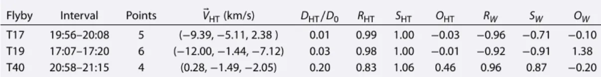
Table 2. Summary of the Walén Analysis for T17, T19, and T40a
Flyby Interval Points ⃗VHT(km/s) DHT∕D0 RHT SHT OHT RW SW OW
T17 19:56–20:08 5 (−9.39,−5.11, 2.38 ) 0.01 0.99 1.00 −0.03 −0.96 −0.71 −0.10 T19 17:07–17:20 6 (−12.00,−1.44,−7.12) 0.03 0.98 1.00 −0.01 −0.92 −0.91 1.38 T40 20:58–21:15 4 (0.28,−1.49,−2.05) 0.20 0.83 1.06 0.46 0.96 0.87 −0.20
aThe columns show the flyby number, the time interval selected, the number of data points, the deHoffmann-Teller velocity, the ratioDHT∕D0, the correlation coefficientRHT, the deHoffmann-Teller slopeSHT, the deHoffmann-Tellery interceptOHT, the correlation coefficientRW, the Walén slopeSW, and the WalényinterceptOW.
and a well-defined minimum variance direction. As a consequence, MVA provides a good estimate for the normal vector to this plane which, in KSO coordinates, resultŝn = (−0.12, 0.40, 0.91). These results show that the variation in the magnetic field direction (in the same time interval where CAPS observations show an acceleration of the plasma flow) is mainly restricted to a plane and can be related to the existence of a one-dimensional current layer. MVAs of MAG data are also performed for flybys T17 and T19. The results are shown and discussed in the next section.
4. Summary and Discussion
In the present study we identify and characterize the progressive plasma acceleration observed at Titan’s induced magnetotail region. These analyses have been based on CAPS, RPWS, and MAG measurements obtained during flybys T17, T19, and T40. Studies of the ion fluxes as well as their angular distribution, mass composition, and energy spectra show consistently that this plasma is mainly composed of two ion populations traveling at approximately the same speed: one with masses ranging from 15 to 17 amu and another one with masses ranging from 28 to 31 amu. During all three flybys the plasma speed in Titan’s wake takes values from about 9 km/s to about 20 km/s. These results are in agreement with the INMS ion com-position observed at Titan’s topside ionosphere [Westlake et al., 2012] and suggest that this plasma has an ionospheric origin. Additionally, RPWS observations show that in these regions of cold plasma the electron density ranges between 0.1 and a few tens of electrons per cubic centimeter. A relative abundance of the two main mass group of ions (mass 15–18 and mass 28–31) has been computed and shows that the con-tribution of these two ion populations varies between 1/3 and 1/2 to the escape with a spatial/temporal variations. Based on the electron number density measurements and plasma speed results, we derive aver-age values for the ionospheric flux flowing away from Titan. In the case of flyby T17, this flux varies between 8.72 × 10⁶ions cm−2s−1and 9.94 × 10⁶ions cm−2s−1. For T19, it varies between 5.05 × 10⁶ions cm−2s−1
and 9.05 × 10⁶ions cm−2s−1; while for T40 it ranges between 2.49 × 10⁶ions cm−2s−1and 4.96 × 10⁶ions
cm−2s−1. The resulting fluxes are close to the ones derived by Sittler et al. [2010]. Assuming a simplified
cylindrical wake with radius ∼ 2.5 RT[Modolo et al., 2007b], the ion escape ranges between 1.1 × 1025ions s−1and 1.3 × 1025ions s−1for T17, it ranges between 6.6 × 1024ions s−1and 1.2 × 1025ions s−1for T19 and it
ranges between 3.2 × 1024ions s−1and 6.5 × 1024ions s−1for T40. We note that these estimations are larger
than the total plasma outflow deduced from the Voyager 1 observations [Gurnett et al., 1982] but are close to other Cassini estimates: 1025ions s−1[Wahlund et al., 2005], (2–7) ×1025ions s−1[Modolo et al., 2007b],
1.7 × 1025ions s−1[Cui et al., 2010], and (2.3, 4.2) × 1024ions s−1[Coates et al., 2012].
Several acceleration mechanisms have been proposed to explain the presence of ionospheric populations in the downstream region of Titan [Edberg et al., 2011]. Among them, magnetic tension forces are expected to be significant at Alfvénic structures. In order to see if the changes in the energy of the plasma might be explained in terms of these forces, we perform tests of the Walén relation. To do this, we first derive the plasma bulk velocity and the local Alfvén speed in Titan’s downstream region taking into account the nec-essary corrections related to the spacecraft potential and velocity. The low values of the ratios DHT∕D0and
the proximity of the correlation coefficients RHTto unity (see Table 2) allow us to identify an approximate HT
frame associated for each of the three flybys studied. Figures 5–7 display their associated Walén plots. As a result, a quasi-stationary pattern of magnetic field and plasma velocity is likely to be present in the down-stream region of Titan. Therefore, the observed time variation in these events is due to the steady motion of the pattern relative to the instrument frame.
In agreement with the Walén relation, we find a linear dependence between the plasma bulk velocity (trans-formed into the HT frame) and the local Alfvén velocity. We determine that the Walén slopes associated
Figure 6. Walén plot corresponding to flyby T17: Walén slopeSW=
(−0.71 ± 0.57),yinterceptOW=(−0.10 ± 0.91)km/s, andR2= 0.92.
with flybys T17, T19, and T40 are (−0.71 ± 0.57), (−0.91 ± 0.17), and (0.87 ± 0.22), respectively. The cor-responding y intercept values are (−0.10 ± 0.91) km/s, (1.38 ± 1.41) km/s, and (−0.20 ± 1.49) km/s. The difference in the sign of the slopes is in agreement with the location of Cassini in Titan’s away or toward magnetic lobes. Dur-ing flybys T17 and T19 the spacecraft is located in the toward lobe where the component of the magnetic field parallel to the flow points in the oppo-site direction to the XTIIS, while in the case of T40 both vectors (magnetic field and velocity) are pointing in the same direction. The uncertainty in the derived slopes and y intercepts are due to experimental uncertainties in the determination of the direction of the flow as well as its energy. The results from flybys T19 and T40, which show relative errors in the slopes of 0.19 and 0.25 are such that both slopes values −1 and +1 are possible. Flyby T17 has a relative error of 0.8 due to the fact that the plasma velocity in the HT reference frame is consid-erably lower than in the previous two cases. As a result, the relative error increases significantly. In spite of this, the results associated with T17 are in agreement with the ones from T19 and T40. When it comes to the y intercept values, the experimental uncertainties allow the possibility that each straight line crosses the origin of coordinates.
We also study the fraction of the total variance present in the y measurements (of each Walén plot) that can be explained in terms of the linear fit model taking as a proxy the value of R2since
R2= 1 − ∑M i=1( yi− fi)2 ∑M i=1( yi−< y >)2 = 1 − ∑M i=1( yi− fi)2 M (std( y))2 (8)
Figure 7. Walén plot corresponding to flyby T19: Walén slopeSW=
(−0.91 ± 0.17),yinterceptOW=(1.38 ± 1.41)km/s, andR2= 0.81.
where< y >= 1 M
∑M
i=1yi, fi = a xi+ b and the values of a and b are the ones obtained through the linear fits. The R2
coefficients for flybys T17, T19, and T40 are 0.92, 0.81, and 0.91, respectively. Noticeably, flybys T17 and T40, charac-terized by R2values higher than T19,
show a closer agreement between their
yintercept and the behavior predicted by the Walén relation.
Moreover, we calculate the correlation coefficients between the slope and the
yintercept derived from the linear fits. The corresponding values for flybys T17, T19, and T40 are −0.35, 0.39, and 0.35, respectively. Even though there is no reason to expect a linear depen-dence between both parameters (as, in fact, it can be seen from these values), the sign of the correlation coefficient
allows us to determine if a and b tend to lie simultaneously on the same or on opposite sides of their respec-tive means. Since flybys T17 and T19 are negarespec-tively/posirespec-tively correlated, decrements in a are correlated to increments/decrements in b. In the case of flyby T40 (positively correlated), increments in a are correlated to increments in b. These results support the closeness between the observations and the theoretical model. Another important aspect to take into account is that several factors could lead to a deviation of the con-stant of proportionality between v′and v
Aand the expected ±1 value: effects of pressure anisotropy, inclusion of data in which the plasma has not yet interacted with the current layer, or unknown contribu-tions to the tangential stress balance not accounted for. Because of these reasons, a proportionality in the range ± (0.8–1.0) is interpreted as a reliable indicator of the presence of an Alfvénic structure [Khrabrov and
Sonnerup, 1998]. In agreement with the existence of such structure, we find that the perturbations of the
magnetic field (ΔB = B − Bo) are close to be perpendicular to the background magnetic field (Bo) during the analyzed time intervals.
Additionally, we perform a MVA of the magnetic field measurements associated to each of the three analyzed flybys to determine if they show signatures which can be associated with the existence of one-dimensional current layers. The ratio𝜆2∕𝜆3results 4.5, 7.26, and 11.45 for the case of flyby T17, T19, and T40, respectively. Therefore, MVA shows a well-defined minimum variance direction and a well-defined intermediate/maximum variance plane for each of the three studied flybys. As a result, MVA provides a good estimate for the normal vector to this plane in the three cases: for the flyby T17, the mean magnetic field vector is< B >= (1.68, 2.22, −1.18) nT (in KSO coordinates) and ̂n = (0.61, 0.67, 0.43). In the T19 case, the mean magnetic field vector is< B >= (−1.06, 3.12, −5.79) nT and ̂n = (0.14, 0.19, −0.97). Finally, in the T40 case, the mean magnetic field vector is< B >= (0.19, 2.07, −1.91) nT and ̂n = (−0.12, 0.40, 0.91). These results show that the variation in the magnetic field direction (for MAG data corresponding to the same time interval where CAPS observations show an acceleration of the plasma flow) is mainly restricted to a plane (intermediate/maximum variance plane), and therefore, they might be associated with the existence of a one-dimensional current layer supporting the proposed acceleration mechanism.
In summary, these results show that the plasma under study is mainly composed of ions also found in Titan’s gravitationally bound ionosphere. According to the performed Walén tests, slope and y intercept values are not so far from what is predicted by theory. Moreover, MVA of the MAG data corresponding to the three fly-bys also show signatures that can be associated with the existence of current layers. Therefore, the observed changes in the kinetic energy might be associated with magnetic tension forces.
Appendix A: Walén Relation
The consistency of the Walén relation and the MHD equations are shown here. For a similar approach, see
Alfvén [1963]. Consider the Navier-Stokes and the magnetic induction equation: 𝜕v 𝜕t + (v⋅ ∇)v = (∇ × B) × B 4𝜋𝜌 − ∇p 𝜌 (A1) ∇ × (v × B) − 𝜕B 𝜕t = 0 (A2)
where the displacement current has been neglected and the plasma conductivity is infinite.
The magnetic field consists of a magnetic field B0generated by currents outside the fluid under study (∇ × B0 = 0) and an induced field b produced by currents observed in the system under study. The total magnetic field is B = B0+ b. In the case of an incompressible fluid (∇⋅ v = 0) with constant density 𝜌
∇ × (v × B) = (B⋅ ∇)v − (v ⋅ ∇)B (A3) Equation (A1) can be rewritten as
( B0 4𝜋𝜌⋅ ∇)b − 𝜕 v 𝜕t = − (∇ × b) × b 4𝜋𝜌 + (∇ × v) × v + 1 𝜌∇ [ p +𝜌v 2 2 + (B⋅ B0) 4𝜋 ] (A4) while equation (A2) can be rewritten as
(B0⋅ ∇)v − 𝜕b
In the case where the sum of the thermal pressure and the magnetic pressure is constant, an exact solution can be found where the fluid velocity and the magnetic field generated by currents inside it are related by the following equation:
v = ±√b
4𝜋𝜌 (A6)
In this case, equations (A4) and (A5) are reduced to (√∓B0
4𝜋𝜌⋅ ∇)b − 𝜕
b
𝜕t = 0 (A7)
Therefore, in the reference frame where
𝜕b
𝜕t = 0 (A8)
the plasma velocity is v′= v − V
ss′, where Vss′= ∓ B0 √ 4𝜋𝜌. Thus, v′= ±√b 4𝜋𝜌 ±√B0 4𝜋𝜌 = ±√B 4𝜋𝜌 = ±vA (A9)
Note that in this reference frame the convective electric field is zero. This equality, known as the Walén rela-tion, states that the bulk velocity of the plasma (seen from a reference frame where the convective electric field is zero) is equal to minus or plus the local Alfvén velocity.
References
Alfvén, H. (1963), Cosmical Electrodynamics, Int. Ser. of Monogr. on Phys., Clarendon Press, Oxford, U. K.
Coates, A. J., F. J. Crary, D. T. Young, K. Szego, C. S. Arridge, Z. Bebesi, E. C. Sittler, R. E. Hartle, and T. W. Hill (2007), Ionospheric electrons in Titan’s tail: Plasma structure during the Cassini T9 encounter, Geophys. Res. Lett., 34, L24S05, doi:10.1029/2007GL030919. Coates, A. J., et al. (2012), Cassini in Titan’s tail: CAPS observations of plasma escape, J. Geophys. Res., 117, A05324,
doi:10.1029/2012JA017595.
Cui, J., M. Galand, R. V. Yelle, J.-E. Wahlund, K. Ågren, J. H. Waite, and M. K. Dougherty (2010), Ion transport in Titan’s upper atmosphere,
J. Geophys. Res., 115, A06314, doi:10.1029/2009JA014563.
Dougherty, M. K., et al. (2004), The Cassini magnetic field investigation, Space Sci. Rev., 114, 331–383, doi:10.1007/s11214-004-1432-2. Edberg, N., K. Ågren, J.-E. Wahlund, M. Morooka, D. Andrews, S. Cowley, A. Wellbrock, A. Coates, C. Bertucci, and M. Dougherty (2011),
Structured ionospheric outflow during the Cassini T55-T59 Titan flybys, Planet Space Sci., 59(8), 788–797, doi:10.1016/j.pss.2011.03.007. Edberg, N. J. T., J.-E. Wahlund, K. Ågren, M. W. Morooka, R. Modolo, C. Bertucci, and M. K. Dougherty (2010), Electron density and
tem-perature measurements in the cold plasma environment of Titan: Implications for atmospheric escape, Geophys. Res. Lett., 37, L20105, doi:10.1029/2010GL044544.
Gurnett, D. A., F. L. Scarf, and W. S. Kurth (1982), The structure of Titan’s wake from plasma wave observations, J. Geophys. Res., 87(A3), 1395–1403, doi:10.1029/JA087iA03p01395.
Gurnett, D. A., et al. (2004), The Cassini radio and plasma wave investigation, Space Sci. Rev., 114, 395–463, doi:10.1007/s11214-004-1434-0.
Hartle, R. E., et al. (2006), Preliminary interpretation of Titan plasma interaction as observed by the Cassini Plasma Spectrometer: Comparisons with Voyager 1, Geophys. Res. Lett., 33, L08201, doi:10.1029/2005GL024817.
Khrabrov, A. V., and B. U. Ö. Sonnerup (1998), DeHoffmann-Teller analysis, in Analysis Methods for Multi-Spacecraft Data, ISSI Sci. Rep.
SR-001, edited by G. Paschmann and P. Daly, pp. 221–248, ISSI/ESA, Noordwijk, Netherlands.
Lewis, G., N. Andrè, C. Arridge, A. Coates, L. Gilbert, D. Linder, and A. Rymer (2008), Derivation of density and temperature from the Cassini Huygens CAPS electron spectrometer, Planet. Space Sci., 56(7), 901–912, doi:10.1016/j.pss.2007.12.017.
Modolo, R., G. M. Chanteur, J.-E. Wahlund, P. Canu, W. S. Kurth, D. Gurnett, A. P. Matthews, and C. Bertucci (2007a), Plasma environment in the wake of Titan from hybrid simulation: A case study, Geophys. Res. Lett., 34, L24S07, doi:10.1029/2007GL030489.
Modolo, R., J.-E. Wahlund, R. Boström, P. Canu, W. S. Kurth, D. Gurnett, G. R. Lewis, and A. J. Coates (2007b), Far plasma wake of Titan from the RPWS observations: A case study, Geophys. Res. Lett., 34, L24S04, doi:10.1029/2007GL030482.
Paschmann, G., and B. U. O. Sonnerup (2008), Proper frame determination and Walen test, in Multi-Spacecraft Analysis Methods Revisited,
ISSI Sci. Rep. SR-008, edited by G. Paschmann and P. W. Daly, pp. 65–74, ISSI/ESA, Noordwijk, Netherlands.
Sittler, E. C., et al. (2010), Saturn’s magnetospheric interaction with Titan as defined by Cassini encounters T9 and T18: New results, Planet.
Space Sci., 58, 327–350, doi:10.1016/j.pss.2009.09.017.
Sonnerup, B. U. Ö., and M. Scheible (1998), Minimum and maximum variance analysis, in Analysis Methods for Multi-Spacecraft Data, ISSI
Sci. Rep. SR-001, edited by G. Paschmann and P. W. Daly, pp. 185–220, ISSI/ESA, Noordwijk, Netherlands.
Szego, K., Z. Bebesi, C. Bertucci, A. J. Coates, F. Crary, G. Erdos, R. Hartle, E. C. Sittler, and D. T. Young (2007), Charged particle environment of Titan during the T9 flyby, Geophys. Res. Lett., 34, L24S03, doi:10.1029/2007GL030677.
Thomsen, M. F., D. B. Reisenfeld, D. M. Delapp, R. L. Tokar, D. T. Young, F. J. Crary, E. C. Sittler, M. A. McGraw, and J. D. Williams (2010), Survey of ion plasma parameters in Saturn’s magnetosphere, J. Geophys. Res., 115, A10220, doi:10.1029/2010JA015267.
Wahlund, J.-E., et al. (2005), Cassini measurements of cold plasma in the ionosphere of Titan, Science, 308(5724), 986–989, doi:10.1126/science.1109807.
Westlake, J. H., et al. (2012), The observed composition of ions outflowing from Titan, Geophys. Res. Lett., 39, L19104, doi:10.1029/2012GL053079.
Wilson, R. J., F. Crary, L. K. Gilbert, D. B. Reisenfeld, J. T. Steinberg, and R. Livi (2012), PDS user’s guide for Cassini Plasma Spectrometer (CAPS).
Young, D. T., et al. (2004), Cassini plasma spectrometer investigation, Space Sci. Rev., 114, 1–112, doi:10.1007/s11214-004-1406-4.
Acknowledgments
The authors thank Cassini CAPS , RPWS, and MAG teams for providing the data used in this study. Please contact the corresponding author ([email protected]) for data access. N.R. is supported by a PhD fellowship from CONICET. The research at the University of Iowa was supported by NASA through contract 1415150 with the Jet Propulsion Laboratory. The RPWS Langmuir Probe is supported by the Swedish National Space Board (SNSB). R.M., J-J.B., F.L., P.C. are indebted to program “Soleil Héliosphère and Magnétosphères” of CNES, the French space administration, for the financial support on Cassini. N.R., R.M. and C.B. are indebted to the ECOS-MYNCYT cooperation program for their support.
Michael Liemohn thanks the reviewers for their assistance in evaluating this paper.