Inclinometry and geodesy: an hydrological perspective

HAL Id: hal-00710444

https://hal.archives-ouvertes.fr/hal-00710444

HAL is a multi-disciplinary open access archive for the deposit and dissemination of sci-entific research documents, whether they are pub-lished or not. The documents may come from teaching and research institutions in France or abroad, or from public or private research centers.

L’archive ouverte pluridisciplinaire HAL, est destinée au dépôt et à la diffusion de documents scientifiques de niveau recherche, publiés ou non, émanant des établissements d’enseignement et de recherche français ou étrangers, des laboratoires publics ou privés.

Inclinometry and geodesy: an hydrological perspective

Laurent Longuevergne, Nicolas Florsch, Frédéric Boudin, T. Vincent, M.

Kammenthaler

To cite this version:

Laurent Longuevergne, Nicolas Florsch, Frédéric Boudin, T. Vincent, M. Kammenthaler. Inclinometry and geodesy: an hydrological perspective. GGP Workshop, 2006, Jena, Germany. pp.11387-11398. �hal-00710444�

Inclinometry and geodesy: an hydrological perspective Proceedings of GGP Workshop, Jena, March 27-31 2006

Laurent Longuevergne1 2, Nicolas Florsch2, Fr´ed´eric Boudin3, Thierry Vincent4, Michel Kammenthaler4

Abstract

Two orthogonal, precise and low drift tiltmeters have been installed in the Vosges mountains in order to study environmental surface loading. The first results show the great sensitivity (10−10

radians), stability (negligible drift) of the instrument, and its ability to be used as a tool to study hydrological loading. This work focuses on local and regional hydrological physical modelling, with a stepwise refinement of mass balance calculations on a geodetic purpose. We show that meteoro-logical forcing mainly drives stock variations inside a hydrometeoro-logical unit, it is therefore necessary to take great care of precipitation and evapotranspiration. Uncertainty assessment on stock variations is also raised, and shows that hydrological models bring good estimation of short term water stock vari-ations, but that long term geodetic variations provide complementary information for stored water modelling.

Keywords : tiltmeter, catchment, hydrological modeling, precipitations, evapotranspiration,

uncertainty assessment.

1_{Corresponding author, E-mail: laurent.longuevergne@ccr.jussieu.fr} 2

UMR Sisyphe, Universit´e Pierre et Marie Curie, Paris, France

3

Institut de Physique du Globe, Paris, France

4

1

Introduction

TheGGP Workshop on analysis of geodetic data geodynamic signals and environmental influences, which took place in Jena in March 2006 showed the growing interest of the geodetic community to understand hydrological contribution on geodetic signals. Several different approaches to the problem have been presented, depending on the goal of the study:

A geodetical approach:

• remove hydrological noise from time series in order to search out external and internal dynamical phenomenon (Kroner et al., this issue),

• validate satellite-derived gravity observations with ground observations, in this case, only local contribution has to be removed (Hinderer et al., this issue).

A hydrological approach:

• Provide a complementary tool to study local and regional hydrology, indeed geodesy is a ”direct” measurement of total mass variation of water (Naujoks et al., this issue),

• validate global hydrological models in the case of GRACE measurements (Neumeyer et al., this issue).

If points of view are various, we are confronted to the same difficulties. First, the question of spatial scales to be taken into account is inseparable of environmental signals (Llubes et al., 2004) since meteorological forcings are distributed on the earth surface. Another difficulty, for local scale in particular, is the way of describing the complex nature of stored water variations with sufficient precision and only a few measurements. Several lines of research have been explored:

• Study correlations between environmental observations and calibration on geodetic data. The problem is that correlation does not give a satisfactory systematic description of hydrological con-tributions, since it depends on the phenomena that are integrated in the study (Tervo et al., this issue). Generally, environmental signals are mixed and correlated - in particular annual signals. • Extract global signal thanks to data processing, using a set of observations at different locations

(Crossley et al., this issue).

• Isolate hydrological processes and understand water flow, by implementing full scale tests (Kroner et al., 2004) or by measuring stored water with an independent method (K¨ugel et al., this issue). • using hydrological models (Krause et al., this issue), for each spatial scale. This is the most

difficult solution, but allows to answer to a lot of questions (for example, separation of spatial scales (Virtanen et al., this issue), etc)

This work opts for physical modelling and is illustrated by tilt data collected by a new in-strument installed in the Vosges Mountains. A stepwise refinement of water mass balance calculations is applied on regional stored water variations, and could be extended to local modelling. Physical processes are first described - in particular hydrometeorological forcings that drive mass balance equation. Then conceptual hydrological models are introduced in order to describe more accurately mass variations. Finally, uncertainty assessment on stock variations is raised.

Table 1: Order of magnitude of the regional hydrological contribution in Sainte-Croix-aux-Mines Phenomenon Time span Equivalent water height [ mm ] Amplitude [ nrad ]

Storm 1 hour 20 20

Winter rainfall 1 day 20 20

Beautiful days 1 week −20 −5

Catchment stocking-destocking 1 year 200 50

Instrument resolution 1 measure 0.1 0.1

2

Tiltmeter: a privileged instrument for surface loading studies

2.1 Scale invariance of tilt deformation field

Tiltmeters are a privileged geodetic instruments for studying surface loading since they are sensitive to all local, regional and global scales (Rerolles et al., 2006). In this sense they are a little different from gravimeters that are only sensitive to global and local scales (Llubes et al., 2004).

For instance, an analytical solution of tilt loadingT can be calculated from green tilt functions (Pagiatakis, 1990), for local and regional scales (see figure 1) when dealing with a full layer water∆h loading uniformly a ribbon which width is b at a distance r of the instrument||T || = 2.k(0).∆h.ln(1 + b/r) . The tilt effect can be written as a separated function of the mechanical behavior of the crust k(0), the geometry of the ribbon and the equivalent height of a full water layer. The scale invariance is illustrated by this example since the deformation is linked to the ratio between the surface and the distance of the loading mass.

In table 1 we can see that hydrology induces geodetic signals at all time scales. Moreover, 1 mm rainfall is equivalent to a 1 nrad tilt deformation because precipitation are concentrated in the bed of the valley. For longer term variations, the whole valley should be taken into account. Notice that the 10−10nrad resolution of the tiltmeter that has been installed is at least 1 order of magnitude better than awaited deformations due to hydrology.

Figure 1: Top view of surface loading on a valley. .

2.2 New tiltmeters installed for this study

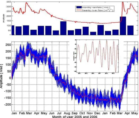
Two orthogonal hydrostatic long base tiltmeters designed by Frederic Boudin from IPGP have been installed in an old mine in the Vosges Mountains, right in front of BFO observatory. Figure 2 shows the hourly and daily raw data of the tiltmeter. No drift can be extracted from this data for the moment, and this is due to the perfect coupling that has been achieved between rock and instrument.

Observed monthly rainfall and water flow of a nearby river are also presented. We can see poor correlation between observed tilt signal and rainfall. On the contrary, tilt is really close to the water flow of the nearby river since water flow is an integrative measurement of the amount of water in a system - what geodesy sees too. During last winter, there was a really poor precipitation rate. Precipitation only occured in March, that’s why tilt - and water flow - signals did not get higher before the beginning of March.

Figure 2: Above: Monthly rainfall and water flow of a nearby river. Underneath: First-year measure-ments (decimated hourly and daily data from 30sec data).

3

Modelling hydrology on geodetic purpose

3.1 Mass balance

3.1.1 Definition of an hydrological unit

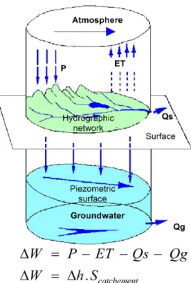
Before mass balance equation is used, an hydrological unit should be defined: the catchment, which is first designed as a topographic catchment (see figure 3). As a consequence, we are almost sure that each water drop falling within the catchment frontier goes out at the single outlet i.e. the gauging station. Mass balance∆W can be written as ∆W = P − ET R − Qs − Qg, where P is precipitation, ETR is real evapotranspiration, Qs and Qg are respectively surface flow and groundwater flow out of the hydrological unit. On the one hand, rainfall and surface flow can be measured, real evapotranspiration can be evaluated; on the other hand, groundwater flow is difficult to measure or evaluate, but represents around 2 to 10% of surface flow, so for the moment, it can be neglected. Hydrologists are used to distribute this stock∆W on the catchment area Scatchement, so stock is expressed as an equivalent full water layer∆h in millimeters, or, it is the same, in kilograms per square meter. Next subsections present major difficulties in calculating mass balance in a catchment.

The Liepvrette catchment (see figure 3) is 100 km2

. The presence of snow caps should be noted and need a special modelling tool in order to take into account this mass of water that does not

Figure 3: Topography of the Liepvrette valley. Both arrows show the directions of the 2 tilt-meters. The Black line rounding the summits is called the topographic catchment, its single outlet (red triangle) is equipped with the gaug-ing station. Superposed isolines 100 days cu-mulative rainfall in mm, used rain gauges seen as blue triangles.

Figure 4: sketch showing water circulation at catchment scale and associated mass balance equation.

stream immediately (Degree day, HBV tool, etc ). One other important property is the 1 day concen-tration time, i.e. the mean time, fallen precipitation take to escape from the catchment. This time limit separates transient and quasi-static behavior of the hydrologic system.

3.1.2 Precipitation variability

One major uncertainty in catchment hydrology is the variability of precipitation field, which is significant in mountainous areas. Figure 3 shows 100 day total precipitations and its variability over the catchment. In this case, a single measure near the instrument underestimates the precipitation near the crest of40%, and so induces a20% mass loss in the balance.

3.1.3 Evapotranspiration

Another difficulty is dealing with evapotranspiration. From observed meteorological forcing (temper-ature, wind speed, insolation ) potential evapotranspiration (PET) can be estimated using different ap-proaches: temperature methods (e.g. Thornthwaite formula), radiation methods (e.g. Turc’s approach) and combination methods (e.g. Penman - Monteith). It is called potential because this calculation rep-resents the evaporing power of atmosphere. Evaluating real evapotranspiration (RET) is then a bit more difficult since it depends on the water available in the soil for the vegetation.

Turc’s law was developed in Western Europe for regions where relative humidity is greater than50%. This law only need information on temperature and duration of insolation. Daily potential evapotranspiration in mm.day−1 _{can be written as} ET P = 0.013 T m

T m+15.(Rg + 50) where T m is the mean daily temperature,Rg is the daily global solar radiation in kJ.m−2.day−1 dependent on the duration of insolation and the astronomical solar insolation which can be found in tables. For45 degrees

Table 2: Order of magnitude of potential evapotranspiration in millimeters calculated by Turc’s law and translated for tiltmeters

Summer Winter

Potential evapotranspiration 3 − 4 mm.day−1 0 − 1 mm.day−1 1 nrad.day−1 0 nrad.day−1

Table 3: Annual variation of stored water in millimeters for different evapotranspiration calculations and translated for tiltmeters. RET is estimated using GR4J rainfall-runoff model (see next chapter)

2002 − 2003 5-year mean ET = RET 290 mm 190mm 70 nrad 45 nrad ET = PET 420 mm 230 mm 100 nrad 55 nrad ET = 0 250 mm 80 mm 65 nrad 20 nrad

latitude situations, potential evapotranspiration is 0 to 1 mm a day in winter and 3 to 4 mm a day in summer (see table 2).

This is an important issue because it does change the annual amplitude in stocked water. When calculating mass balance with observed rainfall and water flow, for different evapotranspiration cases (see table 3), great differences are found. For the Liepvrette catchment, a 5-year mean shows that the annual term of water balance is20 % smaller when using real evapotranspiration than potential evap-otranspiration, but twice as important as ignoring evapotranspiration. When dealing with exceptionally dry years, real annual term is30 % smaller when using real evapotranspiration than potential evapotran-spiration, but only20 % greater than without evapotranspiration. Indeed, in summer 2003 no water was available for vegetation to make it evaporate.

3.1.4 Temporal contribution and Water budget

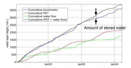
Figure 5 shows the temporal cumulative contribution of each meteorological forcing on water balance. Evapotranspiration is a very annual term, water flow is also annual in opposite phase, but also contains short term variations. The water balance can then be calculated by subtracting the sum of these two last terms and cumulative precipitation. Rainfall brings major part of short term contribution, then, for longer term contribution, evapotranspiration and water flow should be considered. Annual amplitude contributions is presented in table 4.

3.1.5 Stock estimation on geodetical purpose

On a temporal point of view, water balance variations are driven by meteorological forcing. So, it is important to correctly appreciate precipitations and evapotranspiration before starting hydrological modelling. Then, water flow outside the hydrological unit is important because it contains short term as well as long term contribution.

Figure 5: Cumulative temporal contribution of precipitations, evapotranspiration and runoff.

Table 4: Mean annual water budget for Liepvrette catchment. Mean annual rainfall 1100mm

Mean annual PET 700mm Mean annual runoff 500mm Mean annual budget −100mm?

We will show (see figure 8) that a simple calculation of mass balance using sound precipita-tion and evapotranspiraprecipita-tion gives a good first order evaluaprecipita-tion of local or regional water stock variaprecipita-tion in a single hydrological unit.

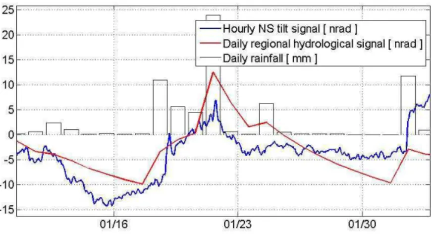
Finally, a geometrical model is necessary to distribute the calculated full layer water height on the hydrological unit. Figure 6 is obtained under the assumption that mass variations are concentrated in the bed of the valley. The discrepancies between the model and observations are certainly due to the fact that internal processes (inside the hydrological unit) of water redistribution are not taken into account.

3.2 Hydrological models

In order to calculate more precisely longer period contribution, real evapotranspiration and ground-water flow should be evaluated, so it is necessary to use hydrological models. This section focuses on catchment modelling. For land surface schemes and soil modelling, please refer to GSWP project http://www.iges.org/gswp/ .

3.2.1 Overview of hydrological models

As far as catchment hydrology is concerned, two kinds of hydrological models can be chosen.

On the one hand, conceptual models describe the global behavior of a catchment using sim-plification of physical processes. Its major advantage is that they contain a few parameters, so they are very robust. Unfortunately it is difficult to extract internal processes because of the poor physical mean-ing of the model. Some models can be cited, dependmean-ing on the major processes that should be taken into account: GR4J (Perrin et al., 2003), Topmodel (Beven et al., 1979), Sacramento (Burnash et al., 1973),

Figure 6: Controntation between observed tilt signal and modelled tilt signal. Note that time sampling is not identical.

HBV (Bergstrm et al., 1973), IHACRES (Jakeman et al. , 1990). A geodetic application was attempted by (Yamauchi, 1987).

On the other hand, physical models can be used. They have a theorical advantage, but contain too many parameters and are not very robust. One other advantage is that these models describe water circulation processes, so the position of the water masses are known. For example SHE (Abbott et al., 1986), SWATCH (Morel-Seytoux et al., 1989). The semi-distributed hydrological model presented by (Krause et al., this issue) is intermediary.

3.2.2 Calibration

Hydrological models are designed to represent catchment behavior at basin outlet, so they are calibrated on stream flow data, and hydrologists traditionally use the nash criteriaF which is a quadratic index (Nash et al., 1970):

F = 1 − Σ(Qobserved− Qsimulated) 2

Σ(Qobserved− E(Qobserved))2

A perfect model is marked 1, a good model is greater than0.6 and F is negative for bad models. A long time serie is often needed, because most information are contained in extreme situations (shallow water, high water, quick streaming, etc)

Hydrologists often adopt a parsimonious behavior towards hydrological modelling because a 3 or 4-parameter model is sufficient to correctly describe stream flow at basin outlet (Beven, 1989, Sorooshian, 1991). Indeed, flow data does not contain all information about internal processes of the catchment (Ambroise, 1991, Grayson et al., 1982).

3.2.3 Application of GR4J rainfall-runoff model

A first experimentation is to apply a conceptual model. For example, GR4J (Perrin et al. 2003) is a 4-parameter model describing flows within a catchment with 2 buckets (so called ”soil” bucket or pro-duction store, and ”groundwater” bucket or routing store), discharge laws and delay laws (see figure 7).

Precipitation is first intercepted (evapotranspiration is subtracted). The soil bucket is then used to calculate real evapotranspiration as a function of the level of the production store. Discharge and / or excess of precipitation is divided into two flow components according to a fixed split:90% is routed by a unit hydrograph UH1 (delay law) and then a non linear routing store (interpreted as groundwater

Figure 7: Left: Description of internal processes of GR4J. Right: Observed and simulated water flow using GR4J

.

Figure 8: Variation of stored water calculated using 3 differents methods. A linear trend has been re-moved

.

store), the remaining10% is routed by a single unit hydrograph UH2 direct to basin outlet. A ground-water exchange term (that can be interpreted as groundground-water flow out of the hydrological unit) is also calculated.

The model has been calibrated on the logarithm of the water flow (see figure 7) in order to describe the annual variations as correctly as possible. Nash criteria is 0.8 which is very good.

3.3 Stored water variations

Stored water within the catchment for 3 cases is shown in figure 8. The blue one is classical mass balance, where processes are respected, but amplitudes are overestimated. The green and red curves are calculated using GR4J rainfall runoff model, either using modelled water flow or observed water flow. We can see the differences, and next question is: Can we evaluate uncertainty on stored water variations?

4

Assessing uncertainties in for stored water variations

This question of uncertainty assessment in hydrological modelling is now a central theme for hydrolo-gists. It is a necessity for two reasons: In terms of likelihood, multimode in model parameter distribution is often observed, and equifinality is often obtained between models when dealing with stream flow data. A few statistical methods exist, for example First-order approximations near global optimum (Kuczera et al.), Generalized Likelihood Uncertainty Estimation (GLUE) method (Beven et al.), Markov Chain Monte Carlo (MCMC) methods (Vrugt et al.), Pareto Optimization Methods (Hoshin et al.). In this work the application of the SCEM-UA algorithm is presented. This is a Bayesian inversion algorithm designed to infer the traditional best parameter set and its underlying posterior distribution by launching parallel Markov chains.

Figure 9 shows the most likely model and the uncertainty according to a 95 % parameter confidence interval. Stream flow is correctly described by the model. One problem is that the observa-tion are seldom inside the uncertainty interval. Two reasons are to be put in an obvious: the fact that uncertainties on observations have not been taken into account, and that a 4-parameter model is unable to provide more information than given in this case.

Figure 9: Most likely model (in blue) and uncertainty associated to water flow modelling (green) accord-ing to a95 % parameter confidence interval. Red dots are water flow measurements.

Figure 10: Most likely model (in blue) and uncertainty associated to modelled stored water variations (green) according to a95 % parameter confidence interval.

When looking to stored water variations (see figure 10), it is interesting to note that short term is correctly described but cumulative errors appear when dealing with stored water variations, particularly in summer if low water stream is not correctly described. In this case geodesy could bring information to longer period variations, for the annual water budget in particular.

5

CONCLUSION

This work focuses on regional (and local) hydrological physical modelling, with a stepwise refinement of mass balance calculations. Water balance variations are driven by meteorological forcings; hence it is important to correctly evaluate precipitation and evapotranspiration. For short term stored water vari-ations (1-2 days), precipitation is a major contributor, for longer term varivari-ations, evapotranspiration and water flow outside the hydrological unit must be taken into account. Simple conceptual hydrological models, calibrated on water flow measurements, allow a more accurate description of nonlinear pro-cesses, i.e. real evapotranspiration and groundwater flow out of the catchment. Uncertainty assessment on stock variations is also raised. It shows that hydrological models bring good estimation of short term water stock variations, and that long term geodetic variations could provide complementary information for stored water modelling.

Acknowledgments:

The authors want to thank Corinna Kroner and the organization staff in Jena for this GGP Workshop. This study, has been carried out within the framework of the ECCO-PNRH program ”Hy-drology and Geodesy”.

References

[1] Abott, M.B., Bathurst, J.C., Cunge, J.A., O’Connel, P.E. et Rasmussen, J. (1986). An introduc-tion to the European Hydrological System - syst`eme hydrologique europ´een, SHE, 1. History and philosophy of a physically-based, distributed modelling system, J. Hydrol., 87, 45-59.

[2] Ambroise, B. (1991). Hydrologie des petits bassins versants ruraux en milieu temp´er´e - processus et mod`eles. S´eminaire du Conseil scientifique du D´epartement Science du Sol de l’INRA Dijon, 26-27 mars 1991.

[3] Bergstr¨om, S. et Forsman, A. (1973). Development of a conceptual deterministic rainfall-runoff model. Nordic Hydrology, 4, 147-170.

[4] Beven, K.J. et Kirkby, M.J. (1979). A physically based, variable contributing area model of basin hydrology. Hydrological Sciences Bulletin, 24(1), 43-69.

[5] Beven, K. (1989). Changing ideas in hydrology - The case of physically-based models, J. Hydrol., 105, 157-172.

[6] Beven, K. (1993). Prophecy, reality and uncertainty in distributed hydrological modelling, Adv. in Water Resources, 16, 41-51.

[7] D.S. Bowles et P.E. O’Conel (eds.), NATO ASI Series C, vol. 345, 443-467, Kluwer Academic Publ.

[8] Burnash, R.J.C., Ferral, R.L. et McGuire, R.A. (1973). A generalized stream flow simulation system - Conceptual modelling for digital computers, U.S. Department of Commerce, National Weather Service and State of California, Department of Water Resources.

[9] Crossley, D., Hinderer, J., Boy, J.P., De Linage, C. (2006): Status of the GGP satellite project, thi issue.

[10] Jakeman, A.J., Littlewood, I.G. et Whitehead, P.G. (1990). Computation of the instantaneous unit hydrograph and identifiable component flows with application to two small upland catchments. Journal of Hydrology, 117, 275-300.

[11] Grayson, R.B., Moore, I.D. et McMahon, T.A. (1992). Physically Based Hydrologic modelling, 1. A terrain-based model for investigative purposes, Water Resour. Res., 28(10), 2639-2658. [12] Hinderer, J., De Linage, C., Boy, J.P.(2006): How to validate satellite-derived gravity

observa-tions with gravimeters at the ground?, this issue

[13] Krause, P., Fink, M., Kroner, C., Sauter, M., Scholten, T. (2006): Hydrological processes in a small headwater catchment and their impact on gravimetric measurement, this issue.

[14] Kroner, C., (2006): Hydrological effects in the SD record at MOXA - a follow up, this issue. [15] K¨ugel, T., Harnisch, G., Harnisch, M., (2006): Measuring integral soil moisture variations using

a geoelectrical resistimeter, this issue.

[16] Llubes, M., Florsch, N., Hinderer, J., Longuevergne L., Amalvict, M. (2004): Local hydrology, the Global Geodynamics Project and CHAMP/GRACE perspective: some case studies, Journal of Geodynamics 38, 355374.

[17] Morel-Seytoux H, Alhassoun S. (1987). SWATCH. Swiss watershed model for simulation of sur-face and subsursur-face flows in stream-aquifer system. Department of Civil Engineering, Colorado State University, 297 p.

[18] Naujoks, M., Kroner, C., Jahr, T., Weise, A.(2006): From a disturbing influence to a desired signal: Hydrological effects in gravity observations, this issue.

[19] Nash, J.E. et Sutcliffe, J.V. (1970). River flow forecasting through conceptual models, 1, A discus-sion of principles, J. Hydrol., 10, 282-290.

[20] Neumeyer, J., Barthelmes, F., Petrovic, S.(2006): Preparation of gravity variations derived form Superconducting Gravimeter recordings, GRACE and hydrological models for comparison, this issue

[21] Pagiatakis, S. D. (1990). The response of a realistic earth to ocean tide loading. Geophys. J. Int. 103: 541-560.

[22] Perrin, C., Michel, C., Andrassian, V. (2003). Improvement of a parsimonious model for stream flow simulation, Journal of Hydrology 279(1-4), 275-289.

[23] Rerolle, T., Florsch, N., Llubes, M., Boudin, F., Longuevergne, L. (2006): Inclinometry, a new tool for the monitoring of aquifers?, Comptes-Rendus de l’acadmie des sciences, accepted. [24] Rodell, M., P. R. Houser, U. Jambor, J. Gottschalck, K. Mitchell, C.-J. Meng, K. Arsenault, B.

Cosgrove, J. Radakovich, M. Bosilovich, J. K. Entin, J. P. Walker, D. Lohmann, and D. Toll (2004), The Global Land Data Assimilation System, Bull. Amer. Meteor. Soc., 85 (3), 381-394, 2004. [25] Sorooshian, S. (1991). Parameter estimation, model identification and model validation:

conceptual-type models. In Recent advances in the modelling of Hydrologic systems,

[26] Tervo, M., Virtanen, H., Bilker-Koivula, M.(2006): Environmental loading effects on GPS time series, this issue.

[27] Virtanen, H., Tervo M., Bilker-Koivula, M.(2006): Comparison of superconducting gravimeter observations with hydrological models of various spatial extents, this issue

[28] Vrugt J.A., H.V. Gupta, W. Bouten, and S. Sorooshian (2003). A Shuffled Complex Evolution Metropolis algorithm for optimization and uncertainty assessment of hydrological model param-eters, Water Resources Research, 2003

[29] Yamauchi, T., (1987) Anomalous strain response to rainfall in relation to earthquake occurrence in the Tokai area, Japan. Journal of Physics of the Earth, 35: 19-36.