Day-Night and Energy Variations for Maximal
Neutrino Mixing Angles
by
Mario Serna
Submitted to the Department of Physics
in partial fulfillment of the requirements for the degree of
Master of Science in Physics
at the
MASSACHUSETTS INSTITUTE OF TECHNOLOGY
June 1999
©
Massachusetts Institute of Technology 1999. All rights reserved.
Author...
Department of Physics
May 7, 1999
I b.Certified by ...
Lisa Randall
Professor
Thesis Supervisor
Accepted by ...
Professor, Associat
Thonas J.
ytak
e Department Head for Education
MASSACHUSETT9 INSTITUTE
Day-Night and Energy Variations for Maximal Neutrino
Mixing Angles
by
Mario Serna
Submitted to the Department of Physics on May 7, 1999, in partial fulfillment of the
requirements for the degree of Master of Science in Physics
Abstract
It has been stated in the literature that the case of maximal mixing angle for ve leads to no day-night effect for solar neutrinos and an energy independent flux suppression of 1. While the case of maximal mixing angle and Am2 in the MSW range of parameter 2
space does lead to suppression of the electron neutrinos reaching the earth from the
sun by Ps = 1, the situation is different for neutrinos that have passed through the earth. We make the point that at maximal mixing, just as with smaller mixing angles, the earth regenerates the
Ivi)
state from the predominantly Jv2) state reachingthe earth, leading to coherent interference effects. This regeneration can lead to a day-night effect and an energy dependence of the suppression of solar electron neutrinos, even for the case of maximal mixing. For large mixing angles, the energy dependence of the day-night asymmetry depends heavily on Am2. With a sufficiently
sensitive measurement of the day-night effect, this energy dependence could be used to distinguish among the large mixing angle solutions of the solar neutrino problem. Thesis Supervisor: Lisa Randall
Acknowledgments
We would like to thank Paul Schechter for a useful conversation. We also greatly ap-preciate Kristin Burgess, Yang Hui He, and Jun Song for reviewing the manuscript. MS would like to thank the National Science Foundation (NSF) for her gracious fellowship, and the Air Force Institute of Technology (AFIT) for supporting this re-search. MS would like to thank Dr. Krastev for helping us understand the parameters involved in calculating the contour plots for the day-night effect. We would also like to thank Robert Foot for useful comments on the manuscript. This work is sup-ported in part by funds provided by the U.S. Department of Energy (D.O.E.) under cooperative research agreement #DF-FC02-94ER40818.
Contents
1 Introduction
2 Review of the Solar Neutrino Problem 2.1 O verview . . . . 2.2 The nuclear reactions in the sun . . . . 2.3 The solar neutrino experiments . . . . 2.4 The missing neutrino flux . . . . 3 The MSW Effect
3.1 Overview of the MSW solution to the solar 3.2 Derivation of MSW equations . . . . 3.3 Validity of the steady state approximation 4 The 4.1 4.2 4.3 4.4 neutrino problem . . . . .
Day-Night Effect at Maximal Mixing O verview . . . . Derivation of Equation (1.1) . . . . Analysis at maximal mixing . . . . Induced energy dependence . . . . 5 Conclusions
A Calculation Methodology for the Day-Night Effect B The Zenith Distribution Function
8 11 11 11 13 14 17 17 18 26 30 30 31 33 35 38 39 43
List of Figures
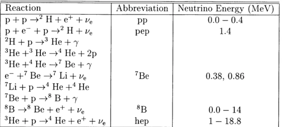
2-1 The solar neutrino energy spectrum, and the experiments sensitive to each reaction. [From Bahcall et. al. in Refs. [6, 81] . . . . 14 2-2 The solar neutrino flux deficit for each of the three types of
experi-ments. The hashed regions indicate the uncertainty in the theoreti-cal estimate or the uncertainty in the measurement. [From Bahtheoreti-call, R efs. [6, 5]] . . . . 15 3-1 MSW Solutions: The shaded areas are regions of the sin2 2 0v - Am2
parameter space that are not excluded (i.e. allowed) by the measured neutrino flux rates of the chlorine, gallium, and water experiments at the 99% confidence level. [From Bahcall, Krastev, and Smirnov in R ef. [12]] . . . . 25 3-2 The regions satisfying the conditions for steady state density matrix.
Above the line (a) is in steady state because of wave packet separa-tion. Above the line (b) can be treated as steady state because of the eccentricity of the earth's orbit. Above the diagonal line (c) is in steady state because the region producing the neutrinos is much larger than an oscillation length, and this phase averaging survives until the
neutrinos reach the vacuum. Above line (d) is in steady steady state because of the energy resolution of our detectors. . . . . 29
4-1 The evolution of P,, as the ensemble of neutrinos propagates across
the center of the earth. The neutrinos enter the earth as an incoherent mixture of the energy eigenstates vi and v2 which is almost completely v2. This plot shown is for Am2 = 1.3 x 10' eV2 and a neutrino energy
E = 6.5 M eV . . . . . 33 4-2 The day-night asymmetry (Ad_, = (N - D)/(N + D)) as a function
of mixing parameters calculated using the density matrix. On the left is a three dimensional surface where the height of the surface is the day-night asymmetry. Notice that the exposed edge is calculated at maximal mixing and is clearly non-zero. On the right is a contour plot showing the lines of constant day-night asymmetry. . . . . 34 4-3 The predicted flux suppression as a function of energy. Notice that the
predicted overall flux suppression is not 1/2, due to day-night effects, even though the mixing angle is maximal. The plot is for Am2 =
1.0 x 10⁻⁵ eV2 which is near the border of the region excluded by the
small day-night effect (Ada) measured at Super-Kamiokande. . . . . 36 4-4 The day-night asymmetry (Ada, = (N - D)/(N + D)) as a function of
recoil electron energy at Super-Kamiokande. Both plots are at maximal mixing angle, with Am2 at the upper and lower borders of the region
disfavored by the smallness of the day-night effect observed at Super-Kamiokande. The rising line is for Am2 = 2 x 10⁻⁵ eV2, and the descending line is for Am2 = 3 x
10-7 eV2. . . . . 37
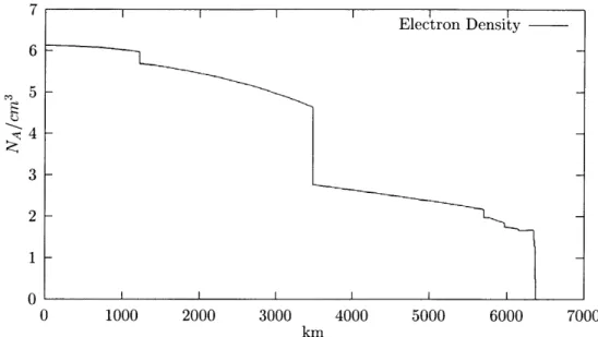
A-i The Preliminary Reference Earth Model (PREM) electron density (Ne)
profile of the earth. Ne is shown in units of Avogadro's number of electrons per cm 3. . . . 40 B-i The zenith distribution function at Super-Kamiokande. . . . . 44
List of Tables
2.1 The pp chain of nuclear reactions in the sun, and the energy of the resulting neutrinos. . . . . 12
Chapter 1
Introduction
The solar neutrino problem is the discrepancy between the theoretical estimates and the experimental measurements of the solar neutrino flux. This problem has been well established over the past thirty years with three separate types of experiments. Neu-trino oscillations are thought to be a possible resolution to the discrepancy. Through most of the past thirty years theorists have assumed that the neutrino mixing must be small in analogy to the small mixing in the quark sector. The recent Super-Kamiokande announcement that atmospheric neutrinos are nearly maximally mixed has renewed much interest in the possibility that solar neutrinos might also be max-imally mixed. In this document we will consider only two-neutrino mixings, so by "maximal mixing" we are referring to the possibility that the two lightest mass
eigen-states, |vi) and jv2), with eigenvalues m, and m2 respectively (mi < m2), are each
equal-probability superpositions of the flavor eigenstate Ive) (electron neutrino) and some other state Iv,), where Ivx) can be any linear combination of Iv,) (muon neu-trino) and
|v,)
(tau neutrino). Many theoretical models have been proposed to predict the possibility of such maximal mixing (for example, see [27, 19, 18, 42, 28, 22, 333). In this document we are concerned only with the MSW solutions to the solar neutrino problem, first proposed by Mikheyev, Smirnov, and Wolfenstein [48, 39, 40], while the alternative possibility of nearly maximally mixed vacuum oscillations has been considered by other authors [201. The MSW effect results from the neutrino inter-action with matter, causing an enhancement of the conversion process transformingVe into v,. The MSW effect is also capable of driving neutrinos back towards a ve
state after passing through the earth. This process would result in a change in the Ve flux between daytime and nighttime measurements, a phenomenon known as the day-night effect, or more generally zenith angle dependence. Over the past decade there have been extensive studies of the day-night effect [21, 16, 17, 36, 37, 38, 10, 49] which have been mostly concerned with the small mixing angle solutions to the solar neutrino problem. Most of these studies have used the Mikheyev-Smirnov expression [41] to describe the effect of the earth on the solar neutrinos, which we will hereafter refer to as Eq. (1.1):
PSE - Ps - sin2 Ov + P2e(1 - 2Ps)
cos20v
Here PSE is the probability that an electron neutrino originating in the sun will be measured as an electron neutrino after passing through the earth, PS is the probability that an electron neutrino (Ve)) originating in the sun will be measured as an electron neutrino upon reaching the earth, P2e is the probability that a pure Iv 2) eigenstate
entering the earth will be measured as an electron neutrino when it emerges, and Ov is the vacuum mixing angle, defined through
I VI) ve) cos Ov - v)sin v , (1.2a)
Iv2) vx) cos Ov + Ive) sin v . (1.2b)
In the previous studies of the day-night effect several authors have claimed that there is no day-night effect at Ps = . (for example, [10, 17]). We wish to emphasize,
however, that the case of maximal mixing is an exception to this statement. For maximal mixing Eq. (1.1) is ill-defined, since cos20v = 0, and we will show below
that generically there is a day-night effect for this case. Nonetheless, we have no disagreements with either the equations or the contour plots in the aforementioned
papers, which in fact do show non-zero day-night effects at maximal mixing. The purpose of this thesis is to clarify the previous papers, and also to investigate more carefully the role of the day-night effect for maximal mixing. We will show that at maximal mixing PSE 5 , implying a day-night effect and an often overlooked energy-dependence of the suppression of the solar neutrino flux.
In the remainder of this document we explain in more detail why maximal mixing can result in a day-night effect. In Chapter 2 we begin with the background of the solar neutrino problem. Chapter 3 then explains the MSW solution to the solar neutrino problem. Next, in Chapter 4, we review the derivation of Eq. (1.1) as given by Mikheyev and Smirnov [41], we resolve the maximal mixing ambiguity, and we present results of numerical calculations showing the day-night effect at maximal mixing. Finally Chapter 5 summarizes the results of the thesis. In the appendices, we provide greater details concerning the numerical calculations presented in Chapter 4.
Chapter 2
Review of the Solar Neutrino
Problem
2.1
Overview
The solar neutrino problem is the discrepancy between the experimental measure-ments and the theoretical predictions of the neutrino flux from the sun. The theo-retical predictions come from models of stellar interiors that calculate the neutrinos generated in nuclear reactions. These models are well-believed and have stood up to robust tests in other contexts. However, direct experimental measurement con-sistently yields a solar neutrino flux significantly below the theoretical prediction. In this chapter we review the major components of the solar neutrino problem: the nuclear reactions involved, the solar neutrino detectors, and the consequences of the missing neutrino flux.
2.2
The nuclear reactions in the sun
Solar neutrinos provide a unique opportunity to see the nuclear reactions in the core of the sun [9]. Because of the high opacity of the solar interior, the photons generated in these regions are heavily scattered and most of the information about the processes which created them has been lost [3]. Neutrinos, however, can relay this information
Reaction Abbreviation Neutrino Energy (MeV) p+p -+2 H+e+ +ve pp 0.0-0.4 p + e- + p -+2 H + ve pep 1.4 2H + p --+ He + 7y 3He + He -7 He + 2p 3He +4 He -+7 Be + 7 e- +7 Be ->7 Li + ve 7Be 0.38, 0.86 7Li + p -+74 He +4 He 7Be + p --8 B + -Y 8B - 8 Be + e+ + v 8B 0.0- 14 3He+p -+4 He + e+ + ve hep 1-18.8
Table 2.1: The pp chain of nuclear reactions in the sun, and the energy of the resulting neutrinos.
since they have an extraordinarily small cross section which allows them to leave the sun almost unaffected. Through models of the solar interior we can predict the quantity and the energy of the neutrinos produced in the sun. These models entail complicated numerical simulations that establish hydrostatic equilibrium between the gravitational force and the thermal pressure from the nuclear reactions, while accounting for opacity, heat transfer, abundance and diffusion of elements. Each of these factors feed back into calculating the rates of all the nuclear reactions which in turn affects the thermal pressure, opacity, and abundances of the elements. The computer code is iterated until a steady state solution is attained. Similar models are used to simulate the complete life of the star. There are two main sequences of nuclear reactions occurring in the solar interior: the pp chain and the CNO chain. The pp (proton - proton) chain dominates the energy production in the sun, while the CNO (carbon - nitrogen - oxygen) chain accounts for only 1% of the total power output of the sun [26]. Table 2.2 shows nuclear reactions in the pp chain and the expected energy range of the neutrinos in these reactions [5, 13]. Fig. 2-1, in the next section, also shows the neutrino energy spectrum from each of these reactions. Measurement of a neutrino flux from these reactions consistent with theoretical prediction would be very strong evidence that our understanding of the physics of the solar interior is correct.
2.3
The solar neutrino experiments
Experiments have been designed and built to measure the solar neutrino flux
[3].
There are currently three main types of experiments; they function by detecting the neutrino reactions in chlorine, gallium, and water. The chlorine experiment(Homestake[23]) relies on the reaction
37CI + Ve -+ e- +3 7 Ar (2.1)
to convert chlorine into argon and is sensitive to neutrino energies greater than 0.9 MeV. The experiment utilizes the fact that argon is a noble gas and can be separated
from the other reactants. The quantity of the isotope 3 7Ar is measured by monitoring its decay. The gallium experiments (GALLEX[29] and SAGE[31]) rely on the reaction
7 Ga + v, e- +7' Ge (2.2)
to convert gallium into germanium and are sensitive to neutrino energies above 0.2 MeV
[7].
Again, one performs the measurement by counting the amount of germa-nium produced after exposing the gallium target to solar neutrinos. The chlorine and the gallium experiments both operate by separating and measuring the products of the reactions after weeks of exposure to solar neutrinos. In contrast, the water exper-iments (Kamiokande[32] and Super-Kamiokande[49]) measure the Cerenkov radiation from the recoil electrons in the scattering reactionve + e~ -- ve + e-. (2.3)
The Cerenkov radiation allows both the energy of the electron and direction of the momentum of the electron to be measured in real time. The energy and momentum vector of the recoil electron in turn provide indirect information about the energy and momentum vector of the incoming neutrino. The water experiments are sensitive to neutrino energies greater than 6.5 MeV. The predicted neutrino energy spectrum and
Chlorine SuperK Gallium I 10"3 10'* 1011
o>
10' 104 10' 101 01 109 . .3 1Neutrino Energy (MeV) Solar neutrino energy spectrum
Figure 2-1: The solar neutrino energy spectrum, and the experiments sensitive to each reaction. [From Bahcall et. al. in Refs. [6, 8]]
the experiments sensitive to the various energy ranges can be seen in Fig. 2-1. These three types of solar neutrino experiments, involving chlorine, gallium, and water, have collected over thirty years of data spanning most of the neutrino energy spectrum.
2.4
The missing neutrino flux
The disagreement between the predicted neutrino flux from the solar models and the measured neutrino flux from the chlorine, gallium, and water neutrino detectors is called the solar neutrino problem. The chlorine experiment measures only 1/3 the theoretically predicted flux, the water experiments only 1/2, and the gallium experiments only 3/5. Fig. 2-2 shows the comparison between the experimental mea-surements and theoretical predictions. The hashed regions indicate the uncertainty in the theoretical estimate or the uncertainty in the measurement. This disagreement is
Total Rates: Standard Model vs. Experiment Bahcall-Pinsonneault 98 7.7+1. 2 -1.0 67±8 .54±0.07 Kamioka SAGE H20 78±6 3ALLEX Ga Theory w 7Be 8B * p-p, pep W CNO Experiments M
Figure 2-2: The solar neutrino flux deficit for each of the three types of experiments. The hashed regions indicate the uncertainty in the theoretical estimate or the uncer-tainty in the measurement. [From Bahcall, Refs. [6, 5]]
0.47±0.02
2.56±0.23
SuperK
the solar neutrino problem; more than thirty years of measurements by three different types of experiments and continual refinement of the solar model with improved cross sections and accounting for smaller order effects have not resolved the disparity.
The disagreement between theory and experiment must mean one of three things: the solar model is incomplete, our understanding of the neutrino cross section is flawed, or something beyond the standard model of particle physics happens to the neutrinos in transit to the earth. Currently, measurements of the speed of sound in the sun (known as helioseismology) lead us to have great faith in the standard solar model [8]. Additionally, variants of the standard solar model also have large disagreements with the measured neutrino flux making it hard to believe that the solar model is the problem. A wide variety of accelerator experiments verify our un-derstanding of particle physics cross sections and the nuclear reactions. Therefore, physicists strongly suspect the mystery lies in what happens to the neutrinos as they travel to the earth. In the standard model of particle physics neutrinos are massless. This means that the flavor eigenstates (Ve, v1, and v,) and the energy eigenstates
can be simultaneously diagonlaized. If neutrinos have non-zero mass then it is pos-sible that the flavor eigenstates would not correspond to the mass eigenstates, and therefore the flavor eigenstates could be superpositions of the mass eigenstates. This superposition of mass eigenstates results in neutrino oscillations. Quantum mechani-cal interference between mass eigenstates oscillating at different frequencies causes a component of the electron neutrino to oscillate into a neutrino of a different flavor. Because the solar neutrino experiments are mostly sensitive to ve measurements, if the neutrinos oscillate into a different flavor then they would pass through the exper-iments undetected. If the lepton mixing mirrors the quark mixing, then one would expect the neutrinos to be only slightly mixed. However, a small mixing leads to only a small fraction of ve oscillating into some other flavor v, and this would not account for the large discrepancy between experiment and theory. Nonetheless, the neutrino oscillation hypothesis is the dominant candidate proposed to solve the solar neutrino problem.
Chapter 3
The MSW Effect
3.1
Overview of the MSW solution to the solar
neutrino problem
The MSW effect, first proposed by Mikheyev, Smirnov, and Wolfenstein [48, 39, 40], allows a small mixing angle to significantly change the fraction of neutrinos arriving at the earth. The effect results from the neutrino interaction with matter which shifts the instantaneous energy eigenvalues of the Hamiltonian. In this high density medium of the solar interior the Ive) state,
Ive) = cos Omlv) + sin OMlv2), (3-1)
is a superposition of the two instantaneous mass eigenstates with a definite phase relationship expressed in terms of the matter mixing angle OM. If the states evolve adiabatically, the fraction of the neutrinos in each adiabatic states, ivi) and jv2),
remains approximately constant. However, in the vacuum the Ive) state is given by a different superposition,
Ive) = cos Ovvi) + sin Ovv 2), (3.2)
expressed in terms of the vacuum mixing angle 0v which is significantly different from
in the vacuum compared to the high density region is responsible for the conversion process transforming ve into v,,, where v., is some neutrino flavor other than ve. This conversion is a possible solution to the solar neutrino problem by enabling some of the ve generated in the sun to be converted into a flavor that is not detected by the neutrino experiments, even with a small vacuum mixing angle.
In this document we are concerned only with the MSW solutions to the solar neutrino problem. The alternative possibility of nearly maximally mixed vacuum oscillations has been considered by other authors [20].
3.2
Derivation of MSW equations
We now present a more detailed derivation of the MSW effect. First we derive the MSW equations of motion for an individual neutrino. We then find the energy eigen-states of the system and use them to find the wave function amplitudes for electron neutrinos produced in the sun and evolved into the vacuum. To describe the ensemble of neutrinos we introduce the density matrix. After averaging out the rapid oscilla-tions we find a steady state solution to the density matrix equaoscilla-tions of motion. We average this solution over the regions of neutrino production.
We begin by finding the MSW equations of motion for an individual neutrino. The coupling describing the interaction between electron neutrinos and electrons is
Hin =V2GFNe, (3.3)
where Ne is the number density of electrons. This contribution to the interaction Hamiltonian is added to the Schr6dinger equation written in the flavor basis. We assume that Ive) can be written as a superposition of only two mass eigenstates, Ivi)
and Iv2). We let Iv.) denote the orthogonal linear combination of Ivi) and Iv2), which
transformation between the vI-v 2 and ve-v, bases is then given by
CL, cos 0v -sin 0v Ce
Cu2) = sinOv cos v
Jk\
CV.)(3.4)
where the variable 0v is the vacuum mixing angle, and C,--
(vIT)
for v = vi, v2, ve or v,. This equation can be written compactly by introducing the index notationCV =UfCV, (3.5)
where the repeated index f is summed over ve and ve, and i is su eigenstates. The Schr6dinger equation for this system is:
C,
P+ 0 (VGFNe0
i8 =t U 2p Ut +
CV. 0 P + Ti 0 0
where we have expanded the energy in the ultra-relativistic limit We now substitute U into the Schr6dinger equation, obtaining
mmed over the mass
I Ci , X (3.6) so that E =+
i
(t
1 2p A A2 sin 20v 2 B v2 GFNe - Aocos 20v, 2 2 (3.7) (3.8) (3.9) (3.10)and where we have dropped the term p+ (+ j + v'GFNe which is proportional to the identity, because terms proportional to the identity cannot contribute to mixing. where
CV, B A
(Cue
The eigenvalues are ±A(N), where A(Ne) = vA 2
+
B2, and the eigenvectors are:V +BT A+B\- (3.11)
(_
= and v+ = ( A .(Since these eigenvectors form the matrix that will diagonalize the interaction matrix in the presence of matter, it is useful to parameterize them by a matter mixing angle
OM (Ne): A-B A+B cos 9 M = , and sinOM = , (3.12) or equivalently A cos 2m = -B, (3.13) or A sin 2M = A. (3.14)
Defining the matrix
cos 0
M sin 0
M
U(6nMMosM - sin Om cos Om 3.15)
the Hamiltonian can be diagonalized as
-A 0 B A
U(O) )Ut (O) = A ) (3.16)
We maintain the notation introduced in Eq. (3.5) so that C ,(OM) Ut (0M)Cvf in
or out of matter, where Cv(OM) = (vilxF) denotes the amplitude for the overlap of the neutrino state with instantaneous mass eigenstates fvi).
To describe the evolution of the neutrinos as they travel to the earth from their creation point in the sun, it is useful to develop the adiabatic approximation, in which one assumes that the density changes imperceptibly within an oscillation length. Remembering that U, OM, and A are all functions of the local electron density Ne, and hence functions of time, we write the Schr6dinger equation in the basis Vi(OM) of
the instantaneous mass eigenstates:
Ct
= A o)(
:D1
+ (iU OtOM (C9)0 A) C V2 CV2
-A 0 C111 0 -aom CV1
0 A) CV2 + tom 0 Cu2
The adiabatic approximation is the assumption that the off-diagonal terms 0X0M can
be neglected, in which case the equation is easily integrated:
(3.19) CV2 (tf)
J+i(t)
CV2(tf) 0 where <(tf) = f A(t)dt. to (3.20)Because the adiabatic states form a complete basis, we can always write the exact solution as a superposition of the two adiabatic states. This final superposition is
expressed by two unknown variables, a1 and a2 where jai1 2 + Ia
21 2
= 1. The ja2 12 parameter represents the probability of a non-adiabatic transition, which is most likely to happen when the neutrinos cross resonance, the density at which B = 0, when the two eigenvalues become nearly equal. Likewise ja1 2 = 1 would represent
adiabatic evolution. Given any initial state vf(to) in the flavor basis, the final state can be written in the general form:
a2
a*
e+i0(tf)
0
0
io))Ut
(om
(to)
Vf(to)-
(3.21)For an electron neutrino originating in a medium of mixing angle Om, the above equation implies that the final state in the vacuum is given by
CV, (tf) A1 a1 cos OMe+i(
+
a2 sin OMeOC (tf) A2
J
--a* cos OMC+e + a* sinOMe-(3.22)
We now go on to talk about the ensemble of neutrinos reaching the earth. To (3.17) (3.18) 0 CV, (to) e-iOett) CV2 (to) CV1 (ty) a, CV2 (tf) )a 2
describe a quantum mechanical ensemble of neutrinos, it is useful to introduce the density matrix
p -
filvi)(vil
(3.23)where
fi
denotes the probability that the particle is in the quantum state Ivi). The density matrix corresponding to a single neutrino as described by Eq. (3.22) is there-fore given by|JA1 2 A1 A*
p = (3.24)
A*A2 |A 2|2
where
AI12= [I + cos 20, ( - 21a 2 12)] + 1 [ala*sin 2me2i4(tf) + c.c] (3.25) A1A* = -sin 20-
[aje2io(tf)
_ -2(t aia2 cos 2 0m (3.26) A212 = [I - cos 20m (I - 21a 22 - [ala*sin 20me2io(tf) + c.c] (3.27) In Sec. 3.3 we explain why this process allows us to eliminate the terms that have rapidly oscillating phases. In particular, the phase angle q(tj) and the phases of thecomplex numbers a, and a2 are all rapidly varying functions of the neutrino energy,
the location in the sun where the neutrino is produced, and the precise time of day and year at which the neutrino is observed. The density matrix which describes the ensemble of observed neutrinos is constructed by averaging over these quantities, so any quantity with a rapidly oscillating phase will average to zero. This is equivalent to the statement that the v, and v2 components arriving at the earth are incoherent,
so we average over their phases. The matrix elements of the phase-averaged density matrix are given by
(JA1 2) = 1+ cos 20M ( - 21a212) (3.28)
(A1A*) = 0 (3.29)
The term la212 - Pjmp is the probability of crossing from one adiabatic state to
the other during the time evolution of these operators. An approximate expression for Pjump can be found by using a linear approximation for the density profile at resonance [43], yielding
Pump = exp - . (3.31)
jump 4p COS(20v)N'(Xres)
Here N(Xres) is the density at the point where the neutrino crosses resonance, and N'(Xres) is the first derivative of the density at resonance. More accurate
approxima-tions to Pjump and the details of their derivation can be found in Refs. [14, 15] and the references therein.
The density matrix corresponding the ensemble of observed neutrinos must be obtained by averaging over the production sites in the sun. While we have already made use of this fact in dropping all terms with rapidly oscillating phases, we must still average the slowly varying terms which remain. Letting 8B(r) denote the normalized
probability distribution for production at a distance r from the center of the sun, one finds finds I+ Co 0 p = 2 0 (3.32) where 1 Rsun Co = - dr 'B(r) cos(20M(r)) (1 - 2jump) (3.33)
Note that the diagonal entries of p are just the fractions k, and k2 of v, and v2 flux
from the sun. Therefore
1 1
ki = - + Co , k2 = - - Co . (3.34)
2 2
Finally, we transform to the ve-vx basis, so
L'e V ~
(Pee
Per 3.5p"""= U(Ov)pUt(Ov ) x PXX (3.35)
P tre Pxx
/
the earth as an electron neutrino is given by 1
PS = Pee = + C cos 20v. (3.36)
2 The off-diagonal matrix element is given by
pe = -Co sin 20v (3.37)
Our numerical simulations have all been performed by integrating Eq. (3.7) to solve for P2e, and also by integrating the density matrix equations of motion. The evolution of the density matrix is given by
ihOtp = -[p, H]. (3.38)
Using Eq. (3.38) with the Hamiltonian in the flavor basis, we find that our new equations of motion are
11OtPee = A(pxe - Pfe) (3.39)
i19tPxe = 2(APee - Bpxe) - A , (3.40)
where A and B are defined in Eqs. (3.9) and (3.10). This allows us to perform calculations using the complete mixed ensemble. The expressions given in Eqs. (3.36) and (3.37) form a steady state solution of the density matrix equations of motion in the vacuum.
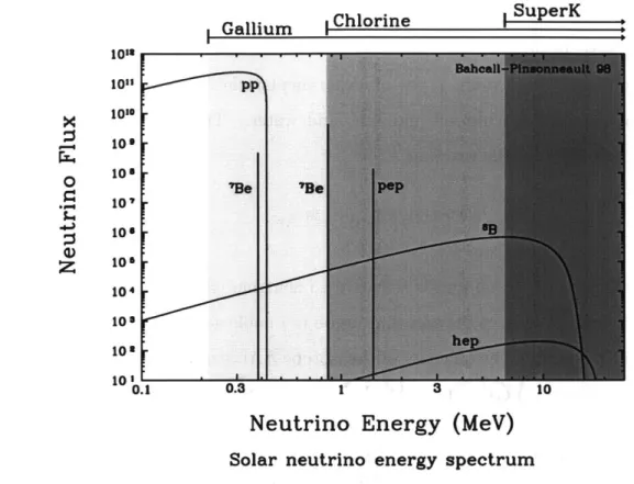
Applying the MSW effect to the neutrinos produced in the sun creates three possible solutions to the solar neutrino problem, pictured in Fig. 3-1. The plot is given as a function of the two basic parameters involved in neutrino oscillations: the vacuum mixing angle expressed as sin2 2 0v and the mass squared difference between
the two mass eigenstates Am2. The shaded areas are regions of the sin2 2 6V - Am2
parameter space that are not excluded (i.e. allowed) by the measured neutrino flux rates of the chlorine, gallium, and water experiments at the 99% confidence level.
10-3 10-4 10-5
,10-6
10-7
ClAr + GALLEX + SAGE
10-8 + SuperKamiokande: rates only SSM: Bahcall and Pinsonneault 1998 10- '
10-4 10-3 10-2 10-1 100
sin2(20)
Figure 3-1: MSW Solutions: The shaded areas are regions of the sin2 20v - 2
parameter space that are not excluded (i.e. allowed) by the measured neutrino flux rates of the chlorine, gallium, and water experiments at the 99% confidence level. [From Bahcall, Krastev, and Smirnov in Ref. [12]]
3.3
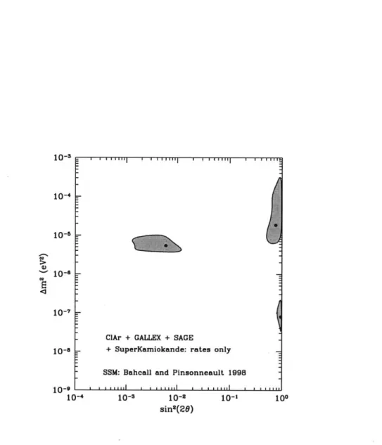
Validity of the steady state approximation
Most of the work in the past decade on the MSW effect has assumed that the en-semble of neutrinos reach the earth in a steady state solution of the density matrix (i.e., in an incoherent mixture of the mass eigenstates vi and v2). There are severalreasons that the neutrinos reach the earth in a steady state: (a) The separation of the IV,) and
|v
2)
wave-packets while propagating from the sun to the earth exceedsthe size of the individual wave packets, eliminating the interference effects. (b) The eccentricity of the earth's orbit results in a daily change of the earth-sun radius larger than the vacuum oscillation length of the neutrinos. (c) The neutrinos are produced in a region much larger than their local oscillation length. (d) The energy resolution of the current detectors coupled with the earth-sun radius perform an average. We now proceed to map out the parameter space justifying where the steady state ap-proximation is valid. First we consider the separation of the two eigenstates during transit to the earth. This results in system that is an incoherent superposition of
lvi)
and IV2).
The width of the wave-packets, or, is given by Ref. [34]:- ~ 0.9 x 10 7 cm. (3.41)
This results in a coherence length given by:
Lcoh - 2 o-/x 2E2 (3.42)
We lose coherence between the mass eigenstates if Lcoh < 1 AU = 1.5 x 101 cm. If we require that the incoherence condition apply up to 14 MeV to include all 8B
neutrinos, we find that for all of sin2 2 0v where Am2 > 6.63 x 10⁻⁶ eV2 the wave-packets have separated upon reaching earth. This corresponds to the region above the line labeled (a) in Fig. 3-2. Because there is a continuous beam of neutrinos arriving from the sun, we can ignore the fact that the lighter mass eigenstate arrives first, and simply drop terms that rapidly oscillate due to the lack of interference between the two states.
In the previous case the interference effects vanish because of a loss of coherence between the mass eigenstates for a neutrino produced at a specific place and time. In the remaining topics the interference effects vanish due to averaging over the ensemble of neutrinos which reach the detector.
Next, we analyze the effect of the eccentricity of the earth's orbit . We are inter-ested in day-night effects; therefore, if the earth-sun radius changes by more than an oscillation length during one day, this will result in washing out any phase dependence in the results measured over a period of one year. Between perihelion and aphelion the earth-sun radius changes by 2e(1 AU) = 5.1 x 1011 cm, where e = 0.017 is the earth eccentricity. The earth-sun radius changes by this quantity once every 180 days giving an average daily change in radius of 2.83 x 109cm. This ensures our incoherent phase for Am 2 > 1.2 x 10⁻⁶ eV2. This region is denoted by everything above the line marked (b) in Fig. 3-2.
Third, we study the impact of where the neutrinos were produced. If the neutrino region of production is greater than the local oscillation length of the neutrinos, then neutrinos of all possible phases exist in the ensemble. For a continuous beam of neutrinos, this also results in dropping the rapidly oscillating terms. The condition is satisfied for the entire parameter space under consideration 0.001 < sin2 20v <
l and 1 x 10-' eV2 < Am2 < 1 x 10⁻³ eV2. However, one must be careful in
making this statement. Although the region of production may be greater than the neutrino oscillation length in the sun, the neutrinos could undergo a non-adiabatic transition, and thus bring a specific phase into dominance. This is the case for vacuum oscillations (Am 2 e 4 x 10⁻¹⁰ eV2). The 8B neutrinos are produced mostly
at R8B= 0.046 R8au = 3.2 x 109cm. The vacuum oscillation length is on the order
of 1 AU. However the oscillations length near the solar core where these neutrinos are produced is about 1.8 x 107cm < R8B. Although the neutrinos are produced in a region larger than their oscillation length, they acquire roughly the same phase in the process of leaving the sun. This occurs because the density change upon leaving the sun occurs more rapidly than the oscillation length of the neutrinos, violating the condition of adiabaticity. To express this quantitatively we estimate that
if Pjump < 0.1 for 14 MeV neutrinos that the initial randomly distributed oscillation phases at the time of production will persist as the neutrinos leave the sun and enter the vacuum. This leads to a steady state solution applicable in the parameter space above the diagonal line labeled (c) shown in Fig. 3-2.
Last, we study the impact of the energy resolution on our ability to discriminate phases. Assuming perfect coherence between the two mass eigenstates the phase upon reaching the earth is given by
Am2(1 AU)
(3.43)
4phc
Our uncertainty in energy impacts our uncertainty in phase through error propaga-tion:
d#Am2(1 AU)
6
60 = do =P - A2( U P. (3.44)
dp 4p2hc
If the uncertainty in our phase is greater than 27r we are again justified in treating our ensemble as a steady state. Using conservative figures for energy (p = 14 MeV), and the energy resolution (6p ~ 1 MeV) [11], we find that for Am2 > 6.5 x 10⁻⁹ eV 2 we are
justified in the steady state approximation. This inequality corresponds to parameter space above the line labeled (d) in Fig. 3-2. Recently Ref. [24] also reached the same conclusions outlined in this section.
Regions Satisfying Steady State Density Matrix 10- 3 10-4 10-5 10-6 10- 7 10-8 10-9 ''I I I .. 10-10 0.001 0.01 0.1 1 sin2 (20v)
Figure 3-2: The regions satisfying the conditions for steady state density matrix. Above the line (a) is in steady state because of wave packet separation. Above the line (b) can be treated as steady state because of the eccentricity of the earth's orbit. Above the diagonal line (c) is in steady state because the region producing the
neutrinos is much larger than an oscillation length, and this phase averaging survives until the neutrinos reach the vacuum. Above line (d) is in steady steady state because of the energy resolution of our detectors.
* I
a:
-... ... ...-... ... -. ... .. ... ...b
Chapter 4
The Day-Night Effect at Maximal
Mixing
4.1
Overview
We have thus far explained the solar neutrino problem, and the MSW solution to the problem. The neutrino interaction with matter can also play a role when the neutrinos pass through the earth. This process would result in a change in the ve flux between daytime and nighttime measurements, a phenomenon known as the day-night effect. Most of the studies of the day-night effect in the past decade [17, 36, 37, 38, 10, 49] have used the Mikheyev-Smirnov expression [41] to describe the effect of the earth on the solar neutrinos, introduced earlier as Eq. (1.1):
Ps-i2 0V + pe(-2s
PSE- PS sin 2 (1 - (1.1)
cos20v
Again PSE is the probability that an electron neutrino originating in the sun will be measured as an electron neutrino after passing through the earth, Ps is the probability that an electron neutrino (Ive)) originating in the sun will be measured as an electron neutrino upon reaching the earth, P2e is the probability that a pure Iv2) eigenstate
entering the earth will be measured as an electron neutrino when it emerges, and 0v
In the Refs. [10, 17] the authors have claimed that there is no day-night effect at
Ps = 1/2. In Eq. (1.1), the properties of the earth enter only through P2e, which is
explicitly multiplied by (1 - 2Ps). We would like to stress that the case of maximal
mixing is an exception to this statement. For maximal mixing Eq. (1.1) is ill-defined, because cos 2 0V = 0. We will now show that at maximal mixing PSE : 1/2, implying a day-night effect and an often overlooked energy-dependence of the suppression of the solar neutrino flux.
Physically, the day-night effect survives because the neutrino beam reaching the earth, for all MSW solutions, is predominantly Jv2). For maximal mixing this state is
half ve and half v2, but there is a definite phase relationship, Iv2) =(Ive)+I v"))/ /2, so
the density matrix is not proportional to the identity matrix. A coherent component of Ivi) is regenerated as this beam traverses the earth, leading to interference with the incident jv2) beam. The case is rather different from the small mixing-angle case, for
which Eq. (1.1) really does imply the absence of a day-night effect when PS = 1/2.
For a small mixing angle Ps equals 1/2 only when conditions in the sun drive the ensemble into a density matrix proportional to the identity matrix, in which case the earth would have no effect.
4.2
Derivation of Equation (1.1)
The key assumption necessary for the derivation of Eq. (1.1) is that the neutrino beam arriving at the earth can be treated as an incoherent mixture of the two mass eigenstates ivi) and jv2). That is, we assume that there is no interference between
the v, and v2 components reaching the earth, or equivalently that the off-diagonal
entries of the density matrix in the v1-v2 basis are negligibly small. The physical
effects which cause this incoherence are discussed in Appendix 3.3. In the case of
maximal mixing, the incoherence is ensured for Am2 > 6.5 x 10~9 eV2 because of the energy resolution of current detectors. Other sources of incoherence include the separation of Ivi) and jv2) wave packets in transit to the earth, the averaging over the regions in the sun where the neutrinos were produced, and the averaging over the
changing radius of the earth's orbit
[24].
In Appendix 3.3 we comment on the regions of parameter space for which the assumption of incoherence is valid.Given the assumption of incoherence, we write the fractions of Iv,) and Iv 2) flux from the sun as k, and k2, respectively. Since there is no interference, the probability
that a solar neutrino will be measured as ve upon reaching the surface of the earth is given by
Ps = ki
I(VeIVI)12
+k2 |VeIV2)12
= k1 cos2 Ov + k2sin2 Ov
= cos2 OV - k2cos 20v , (4.1)
where we have used Eqs. (1.2) and the fact that k, i+k 2 = 1. Similarly, the probability
that a solar neutrino will be measured as ve after passing through the earth, when it is no longer in an incoherent superposition of the mass eigenstates, is given by
PSE - kiPle + k2P2e , (4.2)
where Pie (P2e) is the probability that a Ivi) (Iv2)) eigenstate will be measured as
ve after traversing the earth. Finally, the unitarity of the time evolution operator
implies that the state vectors of two neutrinos entering the earth as Iv,) and |v 2)
must remain orthonormal as they evolve through the earth and become 1'1) and Vi2),
respectively. Therefore
Pie + P2e = (Ve|1)12 + I(Vej22)12 = 1 . (4.3)
Eq. (1.1) can then be obtained by using Eq. (4.1) and the above equation to eliminate
Pie, ki, and k2 from Eq. (4.2).
From the above derivation, one can see that the singularity of Eq. (1.1) at maximal mixing arises when Eq. (4.1) is solved to express k2 in terms of Ps. For maximal
'For large mixing angles, sin2 26V > 0.5 and 5 x 10- < A 2(eV)2 < 1 x 10- 7, k2 e 1 and k, ~ 0.
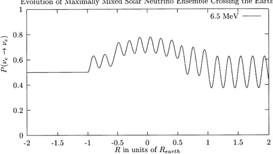
I I 6.5 MeV I -0.8 0.6 -1 -0.5 0 0.5 R in units of Rearth 1 1.5 2
Figure 4-1: The evolution of P,,_, as the ensemble of neutrinos propagates across the center of the earth. The neutrinos enter the earth as an incoherent mixture of the energy eigenstates v and v2 which is almost completely v2. This plot shown is
for Am2 = 1.3 x 10⁻⁵ eV2 and a neutrino energy E = 6.5 MeV.
mixing PS = 1/2 for any value of k2, so k2 cannot be expressed in terms of Ps. The
ambiguity disappears, however, if one leaves k2 in the answer, so Eq. (4.3) can be used to rewrite Eq. (4.2) as
PSE + 2 (k2 )(P 2e-)
2 2 2 (4.4)
Thus, PSE = 1/2 only if k2 = 1/2 or P2e = 1/2. For the MSW solutions at maximal
mixing one has k2 ~ 1, and there is no reason to expect P2e = 1/2. Generically
PSE -f 1/2 for the case of maximal mixing.
4.3
Analysis at maximal mixing
Using the evolution equations derived in Chapter 3 and the procedures described in Appendix A, we have calculated a variety of properties concerning the day-night effect for maximal mixing angle. The calculation parameters are chosen for those of the Super-Kamiokande detector.
Figure 4-1 shows the evolution of P(ve -+ ve), the probability that a solar neutrino ZI
0.4
0.2
0
-2 -1.5
[
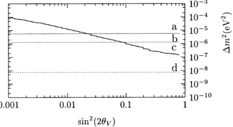
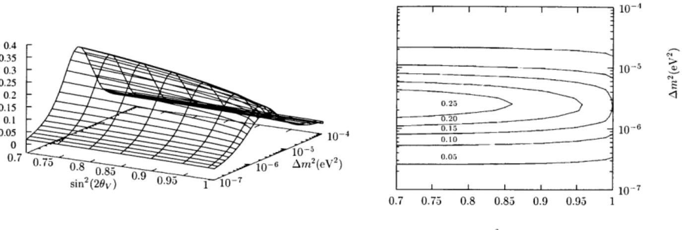
I I I I I i0-~ 0.4 0.35 - 10 0.3 -_ 10-0 0.25 . 0.2 <1 0.15 0.1 .8.20 0.050- 01 10-6 0 sin.8 0 0.95 1 10-7 107 0.7 0.75 0.8 0.85 0.9 0.95 1 sin2 (26v)Figure 4-2: The day-night asymmetry (Ada, = (N - D)/(N + D)) as a function of
mixing parameters calculated using the density matrix. On the left is a three dimen-sional surface where the height of the surface is the day-night asymmetry. Notice that the exposed edge is calculated at maximal mixing and is clearly non-zero. On the right is a contour plot showing the lines of constant day-night asymmetry. will be measured as Ve, as the beam of neutrinos traverses a path through the center of the earth. Notice that after traversing the earth the ensemble of neutrinos is no longer in a steady state, but instead P(ve + ve) continues to oscillate in the vacuum. From the perspective of the mass eigenstates, the neutrinos under consideration arrive at the earth roughly in a jv2) state. Upon reaching the earth, the step-function-like
changes in the electron density profile (see Fig. A-1) cause non-adiabatic evolution, regenerating the Ivi) state and leading to interference effects. In the regions of pa-rameter space where the day-night effect is maximal because the oscillation length of these interference terms coincides with the length of the slabs of near constant density composing the earth, the resulting buildup of ve flux has been called oscillation length resonance [44, 45, 2].
In Fig. 4-2 we present a contour plot calculated from the density matrix that exemplifies the non-zero nature of the day-night effect at maximal mixing. On the left is a three-dimensional surface where the height of the surface is the day-night asymmetry. Notice that the exposed edge is calculated at maximal mixing and is clearly non-zero. On the right is a contour plot showing the lines of constant day-night asymmetry, a plot which is identical to those produced in other references.
4.4
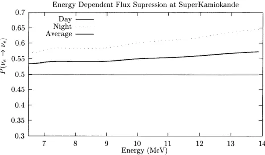
Induced energy dependence
We now explain how the inclusion of the day-night effect at maximal mixing resolves a certain confusion that has arisen in the past because of its neglect. As a result of the non-zero day-night effect, there exists an energy dependence at maximal mixing, as can be seen in Fig. 4-3. If one assumes that the flux suppression at maximal mixing has no energy dependence, as was done in Ref.
[30],
then there is an apparent discrepancy between two sections of Ref. [12]. Sec. IV-D excludes the possibility of energy-independent oscillation into active (as opposed to sterile) neutrinos at the 99.8% confidence level, while Fig. 2 shows some regions of the maximal-mixing-angle parameter space not excluded at the 99% confidence level (we have reproduced Fig. 2 of Ref. [12] as Fig. 3-1 in this thesis). Ref. [30] has tried to resolve this discrepancy without including the day-night effect, concluding that maximal mixing is excluded at the 99.6% confidence level. The actual resolution to this apparent discrepancy is that Fig. 2 of Ref. [12] includes the energy dependence induced by the day-night effect at maximal mixing, while Sec. IV-D discusses the case of energy-independent flux suppression and does not apply to maximal mixing. The correct conclusion is that of Fig. 2, which shows that maximal mixing is not excluded at the 99% confidence level. Whether or not the day-night effect is included, maximal mixing is not a very good fit to the experimental data from the three neutrino experiments (chlorine, gallium, and water) [12]. However, maximal mixing does fit well if the chlorine data is excluded on the suspicion of some systematic error [46]. Ref. [18] has argued that if the 8Bflux is about 17% lower than the standard solar model (BP98) [8], then a bi-maximal mixing scenario becomes a tenable solution to the solar neutrino problem. The MSW mechanism described here is applicable for Am2 > 6.5 x 10- eV2. In the bi-maximal
mixing scenario that we consider the upper bound on Am2 is set by the CHOOZ data
constraining Am2 < 0.9 x 10- eV2 [47].
When detailed studies of the day-night effect are completed, the energy (and zenith angle) dependence will be valuable additional information. To the best of our knowledge, the Super-Kamiokande Collaboration has not published their day-night
0.7 0.65 0.6 0.55 0.5 0.45 0.4 0.35 n3
Energy Dependent Flux Supression at SuperKamiokande Day Night. Average I .- I. .- I. I 7 8 9 10 11 12 13 14 Energy (MeV)
Figure 4-3: The predicted flux suppression as a function of energy. Notice that the predicted overall flux suppression is not 1/2, due to day-night effects, even though the mixing angle is maximal. The plot is for Am2 = 1.0 x 10⁻⁵ eV 2 which is near
the border of the region excluded by the small day-night effect (Ada) measured at Super-Kamiokande.
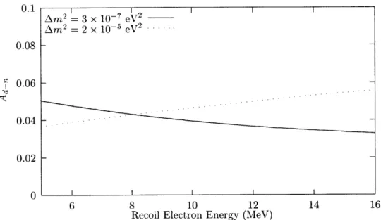
asymmetry as a function of recoil electron energy. Past studies of the day-night effect have noted the energy dependence of the day-night asymmetry [38, 10]. While for small mixing angles jAd-nj < 0.02 without a clear energy dependence [10], for large mixing angles the Ad-, energy dependence can be significant and informative. Fig. 4-4 shows the theoretical predictions of the day-night asymmetry in the electron recoil spectrum at Super-Kamiokande for two cases of maximal mixing: Am2 = 2 x 10- eV2 and Am2 = 3 x 10⁻⁷ eV2. Note that the two curves have opposite slopes.
The approximate shape of the graph of Ad-_ vs. recoil electron energy can be understood from Fig. 4-2, using the fact that Fig. 4-2 is dominated by the peak of the
8B neutrino spectrum at about 6.5 MeV. It is shown in Appendix 3.2 that the neutrino
evolution equations (Eqs. (3.7)-(3.10)) depend on Am2 and the neutrino energy (or momentum) E only through the combination Am2
/E.
Thus, Fig. 4-2 shows that forany value of sin2 20v, Ad-, has a maximum at Am2/E ~ 2.5 x 10⁻⁶
0.1 0.08 i 0.06 -0.04 - -- - - - --- 0.02 0 6 8 10 12 14 16
Recoil Electron Energy (MeV)
Figure 4-4: The day-night asymmetry (Ad-_ = (N - D)/(N + D)) as a function of recoil electron energy at Super-Kamiokande. Both plots are at maximal mixing angle, with Am2 at the upper and lower borders of the region disfavored by the smallness of the day-night effect observed at Super-Kamiokande. The rising line is
for Am2 = 2 x 10⁻⁵ eV2, and the descending line is for Am2 - 3 x 10⁻⁷ eV2.
When E is varied at fixed Am 2, Ad-. will have a peak at
Am2
E I 10I 2 V x 6.5 MeV
. (4.5)
2.5 x 10⁻⁶ eV2
So for Am2 = 2 x 10⁻⁵ eV2 the peak lies far to the right of the scale in Fig. 4-4, so the curve slopes upward. For Am2 = 3 x 10⁻⁷ eV2 the peak lies far to the left, and the curve slopes downward.
Fig. 4-2 shows that the peak in the graph of Ad-_ vs. Am2 is higher at large mixing angles (sin2 2 0v ~ 0.7) than it is at maximal mixing, so the same will be
true for the energy dependence of the day-night effect. For sin2 2 0v = 0.63 and Am2 = 1.3 x 10⁻⁵ eV2, for example, the slope of the graph of Ad_. vs. recoil electron
energy is about twice the magnitude of the slopes shown in Fig. 4-4. Thus, the day-night asymmetry as a function of recoil electron energy could be a strong indicator of Am2 if the solar neutrinos have a large or maximal mixing angle in the MSW range of parameters.
Am 2 = 3 x 10⁻⁷ eV2 Am 2 = 2 x 10⁻⁵ eV2
Chapter 5
Conclusions
In this thesis we have reviewed the solar neutrino problem, and we have derived the MSW solution to the solar neutrino problem. We have also derived the Eq. (1.1) for calculations of the day-night effect. We have pointed out that Refs. [10, 17] incorrectly assume that that Ps = 1/2 always implies PSE = 1/2. We have also shown that neutrinos with a maximal mixing angle can have a day-night effect and that they do not always result in a uniform energy-independent flux suppression of 1/2. Because the issues that we have attempted to clarify concern mainly the words that have been used to describe correct equations (which were generally used numerically), there are no changes to most constraints presented in other references. The only corrections apply to fits of energy-independent suppressions; that is, in contradiction with the assumptions of Ref. [30], the fits do not apply to the exclusion of some regions of maximally mixed neutrinos. Finally, we have noted that the energy dependence of the day-night effect can be a strong discriminator between various solutions of the solar neutrino problem.
Appendix A
Calculation Methodology for the
Day-Night Effect
First we calculated Ps using Eq. (3.36) for the spectrum of Am2
/p
at various mixing angles. For a given Am2/p we averaged Ps over the regions of 'B neutrino productionin the sun, provided by Ref. [6]. Using Ps to describe the neutrinos that arrive at the earth, we then performed the evolution through the earth with the density matrix equations of motion. The initial conditions for the density matrix are given by
Pee = PS, (A.1)
and
1
Pxe (2Ps - 1) tan 26v. (A.2)
2
At maximal mixing we assume that Pxe = cos(20m(to)) sin 20v a
}
which is theadiabatic result. This assumption is justified because in the regions of parameter space under consideration near maximal mixing, jump ~ 0. It follows that in these same regions of parameter space the evolution remains adiabatic in the limit where
0v = 7r/4. We use the earth density profile given in the Preliminary Reference Earth
Model (PREM) [25] (see Fig A-1). To convert from the mass density to electron number density we use the charge to nucleon ratio Z/A = 0.497 for the mantle
7 6 3 2 1 --0 0 1000 2000 3000 4000 5000 6000 7000 km
Figure A-1: The Preliminary Reference Earth Model (PREM) electron density (Ne) profile of the earth. Ne is shown in units of Avogadro's number of electrons per cm3.
and Z/A = 0.467 for the core. The numerical calculations were performed using a fourth order Runge-Kutta integration programmed in C++. We propagated the neutrinos through the earth for 90 zenith angles, a, evenly spaced between 90 and 180 degrees. We calculate the anticipated electron flux as a function of zenith angle and energy, denoted PSE(a, E,). The calculation parameters are chosen for those of the Super-IKamiokande detector. The normalized 8B neutrino spectrum, <b(E,), and
solar electron densities, Ne, are also obtained from data-files provided by Ref. [6]. Effective neutrino cross sections are available which take into account the electron recoil cross section with radiative corrections, the energy resolution, and the trigger efficiency [11, 6]. We used these more accurate cross sections for the overall day-night effect plotted in Fig. 4-2. Because these effective cross sections already include the integration over detected electron recoil energy, to calculate the recoil electron spectrum we used the differential neutrino-electron scattering cross sections given in Ref. [4]. Using these data files and numerical results the cross section for the scattering of solar neutrinos of energy E, with electrons to produce a recoil electron of energy T' at the zenith angle a is given by
+ [1 PSE(a, E,)] T(T', Ev). (A.3)