Assessing the fuel Use and greenhouse gas emissions of future light-duty vehicles in Japan

(1)

Assessing the Fuel Use and Greenhouse Gas

Emissions of Future Light-Duty Vehicles in Japan

by

MASSACHUSETTS INSTITUTE

OF TECHN4OLOGY

Eriko Nishimura

_{JUN 0 7 2011}

Bachelor of Engineering in Mechanical Engineering

-LBRARIES

University of Tokyo, Japan, 2005

Submitted to the Engineering System Division

in partial fulfillment of the requirements for the degree of

Master of Science in Technology and Policy

at the

Massachusetts Institute of Technology

June 2011

©

2011 Massachusetts Institute of Technology. All rights reserved.

Signature of author:

Engineering Systems Division

Technology and Policy Program

May 6, 2011

Certified by:

Jolin B. Heywood

Professor of Mechanical Engineering

Sun Jae Professor, Emeritus

Thesis Supervisor

Accepted by:

Dava J. Newman

Professor of Aeronautics and Astronautics and Engineering Systems

Director of Technology and Policy Program

(2)

(3)

Assessing the Fuel Use and Greenhouse Gas Emissions of Future Light-Duty Vehicles in Japan

by Eriko Nishimura

Submitted to the Engineering System Division on May 6, 2011, in partial fulfillment of the requirements for the degree of Master of Science in Technology and Policy ABSTRACT

Reducing greenhouse gas (GHG) emissions is of great concern in Japan, as well as elsewhere, such as in the U.S. and EU. More than 20% of GHG emissions in Japan come from the transportation sector, and a more than 70% reduction in GHG emissions by 2050 has been projected as a feasible goal. It is clear that substantial reduction in GHG emissions from the transportation sector will be required in Japan over the next several decades.

This research developed a fleet model for Japan to evaluate GHG emission trends through 2030 and through 2050. The fleet model shows that GHG emissions from light-duty vehicles are likely to decrease significantly due to anticipated decrease of vehicle kilometers traveled (VKT) from all the light-duty vehicles in Japan over the next several decades. This is because of several factors, such as the decrease of vehicle sales due to the recession and higher gasoline prices.

In the analysis through 2030, the fleet model was run under four "sales mix scenarios," including a scenario which is based on the forecast by the Japanese Government. Even in the scenario without any sales mix change in the future, a 36% GHG emission reduction from the level of 2008 is achieved by 2030. In the Government Scenario (the most optimistic scenario), a 49% GHG emission reduction from the level of 2008 is achieved by 2030.

In the longer-term analysis through 2050, the fleet model was run under two "sales mix scenarios" and two "vehicle fuel consumption forecasts." In the most conservative case, a 54% GHG emission reduction from the level of 2008 is achieved by 2050. In the most optimistic case, a 67% GHG emission reduction from the level of 2008 is achieved by 2050.

Even though substantial GHG emission reductions by 2050 are projected, coordinated policy measures would make the most optimistic sales mix scenario more feasible, and help realize further GHG emission reductions.

Thesis Supervisor: John B. Heywood

(4)

ACKNOWLEDGEMENTS

This work could not have been completed without the support of many people.

First of all, I would like to express my deepest gratitude to my supervisor, Professor John B. Heywood. He is one of the best advisors I have ever had, and his advice and suggestions were always very helpful. I am fortunate to have found such a wonderful supervisor to work with.

I would also like to thank everyone in the Sloan Automotive Lab at MIT. In particular, I am indebted to Lynette Cheah. Whenever I had problems with my research, she always helped me and gave me numerous ideas and suggestions. Parisa Bastani and I worked together to check the fleet model many times. I am grateful to Valerie Karplus, Don MacKenzie, Kandarp Bhatt, and Stephen Zoepf for their feedback and advice on my work during different stages of this research.

Furthermore, I would like to express my heartfelt thanks to Robert Irwin in the Writing and Communication Center for giving me advice about writing better in English.

Finally, I would like to thank my wonderful husband, Masahiro Ono. He constantly encouraged me, shared his experience as a researcher, and supported me in a multitude of ways.

(5)

LIST OF FIGURES AND TABLES

Figure 1. The kilometers-traveled per person per year of each transportation model ... 11

Figure 2. Fleet model overview ... 14

Figure 3. Vehicle sales in Japan... 15

Figure 4. Vehicle sales projection in Japan ... 16

Figure 5. The survival rates of compact and normal passenger cars ... 17

Figure 6. The survival rates of compact trucks... 17

Figure 7. The trend of average lifetime Japan ... 19

Figure 8. The trend of median lifetime ... 21

Figure 9. The comparison of survival rate curves ... 22

Figure 10. Growth parameter

p

for different years ... ... 23

Figure 11. VKT per vehicle per year ... 24

Figure 12. VKT per vehicle per year by model year (1980-2009)... 25

Figure 13. Sales mix scenarios for standard vehicles... 31

Figure 14. Sales mix scenarios for light vehicles ... 31

Figure 15. In-Use Vehicle Weight Distribution in Japan in 2008 ... 32

Figure 16. Fuel Consumption and Vehicle Weight by JC08 mode in Japan... 34

Figure 17. Japanese test cycles for measuring vehicle fuel economy ... 36

Figure 18. The trend of vehicle fuel consumption for all passenger vehicles ... 37

Figure 19. The trend of vehicle fuel consumption for each vehicle category ... 38

Figure 20. Relative fuel consumption for different propulsion systems ... 40

Figure 21. Vehicle stock (fleet model results compared with historical data)... 42

Figure 22. Vehicle stock for each vehicle category... 43

Figure 23. Total fleet VKT in the future ... 46

Figure 24. Fleet fuel use ... 48

Figure 25. Fleet fuel use for each scenario ... 50

Figure 26. Fleet electricity use ... 51

Figure 27. Fleet electricity use for each scenario ... 53

Figure 28. Electricity generation by source ... 55

Figure 29. Fleet GHG emissions ... 57

Figure 30. Fleet GHG emissions for each scenario... 60

Figure 31. Average light-duty vehicle weight in Japan ... 61

Figure 32. Estimated Survival Rates (model year 2030 onward) ... 65

(8)

Figure 34. Sales mix scenarios for light vehicles ... 69

Figure 35. Relative fuel consumption for different propulsion systems (Gov-based)... 71

Figure 36. Relative fuel consumption for different propulsion systems (U.S.-based)... 71

Figure 37. Vehicle stock through 2050 ... 72

Figure 38. Total fleet VKT through 2050 ... 73

Figure 39. Fleet fuel use through 2050 ... 75

Figure 40. Fleet fuel use through 2050 for each case ... 78

Figure 41. Fleet electricity use through 2050 ... 79

Figure 42. Fleet electricity use through 2050 for each case ... 80

Figure 43. Fleet GHG emissions through 2050 ... 81

Figure 44. Fleet GHG emissions through 2050 for each case ... 83

Table 1. Japanese vehicle categories ... 12

Table 2. Vehicle sales growth projection (growth % per year)... 15

Table 3. Vehicle inspection cost... 20

Table 4. Adjustments for median lifetime ... 21

Table 5. The growth projections for median lifetime ... 21

Table 6. Sales mix of the Government Scenario... 28

Table 7. Sales mix of the Half of Government Scenario ... 29

Table 8. Sales mix of the Realistic Scenario ... 30

Table 9. Average vehicle weight for each vehicle category ... 33

Table 10. Vehicle fuel consumption for each vehicle category of Model Year 2008 ... 38

Table 11. Difference between fleet data and model calculation ... 43

Table 12. Taxes for passenger cars in Japan... 44

Table 13. The scope of data and fleet model... 46

Table 14. Energy use and C02 emission factors ... 54

Table 15. Annual vehicle sales projection (2030-2050) in Japan... 64

Table 16. Assumed median lifetime (2030~2050) in Japan ... 64

Table 17. VKT per vehicle per year projection (2030~2050) in Japan... 65

Table 18. Sales mix of Scenario A ... 67

(9)

1. INTRODUCTION

1.1 Objectives

The overall objective of this research is to quantify the potential future petroleum, energy and environmental impacts of the new and improved technologies and fuels likely to be developed and deployed in light-duty vehicles.

Under the Kyoto Protocol, which was initially adopted on 11 December 1997 in Kyoto, Japan, and entered into force on 16 February 2005, Japan committed to reducing greenhouse gas (GHG) emissions by 6% from the 1990 level during the period between 2008 and 2012. This constituted a very stringent target for Japan because GHG emissions have already increased after 1990. The percentages of GHG emission increase by 2005 from the level of 1990 are 44.6% from the commercial and other sectors, 36.7% from the residential sector, and 18.1% from the transportation sector

[Matsuhashi et al., 2007].

Over the next several decades, substantial reduction in GHG emissions from the transportation sector will be required. The share of GHG emissions from the transportation sector in Japan was 24.4% in 2008 [IEA, 2008]. In particular, more than 80% of GHG emissions of the transportation sector in Japan were derived from vehicles such as passenger cars and trucks in 2006 [Public Relations Division of MLIT, 2008]. As Japan as well as other countries in the world consider how best to set targets for reducing GHG emissions, assessing the opportunities for reducing the transportation

sector's contribution is especially important.

The Japanese government has addressed these issues in five main ways [MLIT, 2007]. First, the Japanese government has been promoting popularization of "environmentally friendly vehicles" such as hybrid and battery electric vehicles. Due to the great efforts by the government, the sales of hybrid vehicles have been growing rapidly over the last several years. Second, the government has set stringent targets for fuel economy based on the best available technology. Third, the government has been working on constructing an "efficient transportation system." Fourth, the government has been trying to introduce "efficient traffic control" and develop infrastructure. Fifth, the government has promoted the use of public transport, such as trains and buses, instead of passenger cars. Since the high gasoline prices (about JPY 150 per liter [The Oil Information Center, IEEJ, 2011]) for the last several years have also helped this

(10)

government policy a great deal, people drive less than they did previously.

Owing to these integrated approaches by the Japanese government, GHG emissions from vehicles have gradually started decreasing. However, it is still unclear what the fleet impacts will be in the future. Therefore, the purpose of my research is to forecast and analyze fuel use and GHG emissions from light-duty vehicles (LDVs: passenger cars and light trucks) in Japan over the next few decades. The analysis is divided into two parts: near future (through 2030) and longer term (2030-2050). In the first part, the results from the fleet model are based on detailed assumptions. In the second part, the results from the fleet model have more uncertainties, but it is useful to have a rough image of GHG emission trends as long-term targets for GHG reductions are considered. 1.2 Overview of Transport in Japan

Japan is a small-size country and the land area is 378 thousand km2_{, which is about 4%} of that of the United States [Statistics Bureau of MIAC, 2010]. However, the population is 128 million, more than 40% of that of the United States [Statistics Bureau of MIAC, 2010]. Because of these differences, the characteristics of transport are quite different from those of the United States.

The number of kilometers-traveled per person per year is given in Figure 1 [Transport Research and Statistics Office, MLIT, 2010]. The demand for railroad is quite high because the modern network of railroads spreads over the whole country including a high speed railroad called Shinkansen. On the other hand, the demand for air transport is relatively low, arguably because of the existence of the high speed railroad and of the small land area. The kilometers-traveled per person by passenger car increased at an annual rate of 2.6% in 1990s, but has recently been decreasing. On the other hand, the kilometers-traveled per person by railroad has gradually been increasing. There are at least three possible reasons for this trend. First, the price of gasoline was high in the latter half of the past decade. Second, the network of railroads has been extending, and the railroad is becoming more convenient for traveling. Third, more and more people are interested in climate change issues. Yet even though people are less dependent on vehicles for traveling in Japan compared with the United States, in 2006 more than 80% of transportation GHG emissions came from road vehicles, including buses and trucks [Public Relations Division, MLIT, 2008].

(11)

(km) Travel km per person per year The ratioof each transport mode 6,000 (2008) 5,000 car 6%) U passenger 4,000 - - - -0-bus

-*-busiH

M

bus

3,000 -3,000___________ _ --&- ra iIroad 3,168km 5,585km 2,000 (31%) (55%) 111 railroad 1,000 -- air 0 i704km NKair 1990 1995 2000 2005 2010 (7%)

Figure 1. The kilometers-traveled per person per year of each transportation model [Transport Research and Statistics Office, MLLT, 2010]

It is therefore appropriate to focus on the road transportation. The categorization of Japanese vehicles, shown in Table 1, is unique. There are three vehicle categories for passenger cars, and three vehicle categories for trucks. For passenger cars, vehicles are categorized based on the size and displacement. First come "K-cars," so called because the pronunciation of K stands for "light" in Japanese. As for trucks, vehicles are categorized based on the size, displacement, and load capacity. The scope of this research is limited to LDVs. That means the first five categories shown in Table 1, and does not include "normal trucks." Normal trucks are excluded for the following reasons. First,, most of the normal trucks are heavy-duty vehicles, which are mainly used not for personal transport but for freight. Second, diesel oil is used for normal trucks in most cases, which is completely different from the trend of light-duty vehicles, which use gasoline in most cases.

(12)

Table 1. Japanese vehicle categories

Vehicle stock Vehicle sales

Vehicle category Defmition

(2009) (2009)

K-car Maximum length: 3.4m (light Maximum width: 1.48m

17.5 million 1.3 million motor Maximum height: 2.Om

vehicle) Maximum displacement: 660cc

passenger Maximum length: 4.7m

cars compact Maximum width: 1.7m

23.7 million 1.6 million car Maximum height: 2.Om

Maximum displacement: 2000cc All passenger cars other than

normal car 16.7 million 1.3 million

above

Maximum length: 3.4m K-truck Maximum width: 1.48m

(light Maximum height: 2.Om 9.2 million 0.4 million

truck) Maximum displacement: 660cc Maximum load capacity: 350kg Maximum length: 4.7m

Maximum width: 1.7m trucks

Maximum height: 2.Om compact

Maximum displacement: 3.9 million 0.2 million

truck

2000cc (except for Diesel and CNG) Maximum load capacity:

2000~3000kg (ambiguous) normal All trucks other than above

(13)

2. FLEET MODEL DEVELOPMENT (through 2030)

2.1 Fleet Model Overview

A quantitative model for assessing the impacts on Japan's GHG emissions of different evolving transportation technologies and fuel scenarios needs the following components: [Heywood, 2010]

(a) A vehicle analysis capability that, for given propulsion system and vehicle technologies, can predict the vehicle's fuel consumption and GHG emissions over specified drive cycles.

(b) A model for the dynamics of the in-use vehicle fleet, which includes vehicle sales and scrappage rates, and annual kilometers traveled.

(c) Specification of new or improved technology introduction timeframes and deployment rates of these technologies as a function of time.

(d) The resolution of the vehicle fuel consumption, performance, and vehicle size trade-off that, for given powertrain and vehicle technologies, affects the improvement in fuel consumption actually achieved.

(e) Quantitative scenarios for the fuel (or energy) streams expected to be available over the appropriate timeframe and the GHG emissions associated with the production and distribution of those fuels.

MIT's Sloan Automotive Laboratory has developed such a methodology for the respective LDV fleets for the United States context [Bandivadekar et al., 2008] and for several major European countries [Bodek and Heywood, 2008]. There is also a similar study by Greene and Plotkin for the U.S. transportation sector [Greene and Plotkin, 2011]. Based on the MIT work, the overall structure of the in-use LDV fleet model is given in Figure 2, which shows the required inputs, and the logical sequence of the outputs: the make-up of the LDV stock; the LDV fleet kilometers traveled; the fleet fuel use; and the fleet GHG emissions. The fleet model is composed of several worksheets in Microsoft Excel. The several components of this methodology will now be reviewed.

(14)

1. Vehicle

2. Survival

a) LDV (Light Duty

Sales

Rate

Vehicle)

stock-Vehicle fleet

modeling

3. Vehicle Kilometers

b) LDV Fleet

Traveled per vehicle

Kilometers Traveled

4. Sales mix

c) LDV

Fleet

Fuel

Scenario

5. Vehicle fuel

Use & Fleet

analysis

consumption

Electricity Use

6. Energy use and

d) LDV Fleet GHG

**CO2 *emission factors**

Emissions

Figure 2. Fleet model overview

2.2 Key Assumptions

Not only historical data but also several other assumptions are required to operate the fleet model. These assumptions, which are described in detail below, include the future growth rate of new vehicle sales, the fuel consumption of new vehicles, and the VKT behavior.

2.2.1 Timeframe (near future: through 2030)

A two-decade timeframe through 2030 was chosen over which to evaluate the results from the fleet model. The timeframe was capped at twenty years because it is very difficult to project improvements in various factors beyond this period. Since analyzing beyond this period involves more uncertainties, near-future analysis is separated from

longer-term analysis.

2.2.2 Sales Projection

The annual sales of LDVs in Japan from 1975-20091 are shown in Figure 3. Here, I considered the number of newly registered vehicles as the number of sales.

(15)

(mu) 8 _-All _LDVs 7 -compact& 6 normal car -- compactcar S5 40 4 -K-car E3 2 2 ... ,...

~

- normal car - -K-truck -. . compact truck 0 1975 1980 1985 1990 1995 2000 2005 2010

Figure 3. Vehicle sales in Japan [AIRIA, 2000, 2009]

The number of LDV sales increased significantly in the 1980s, and the number of total LDV sales was larger than seven million around 1990. However, the number of sales has recently been decreasing in all the vehicle categories except for K-cars. Since the vehicle sales have been decreasing so rapidly, the future vehicle sales trend is projected and shown in both Table 2 and Figure 4, based not on historical data but on the government's sales forecast. More concrete reasons for choosing this approach are as follows. First, if vehicle sales are forecast based on historical data, the sales of compact trucks becomes close to zero in a few years, which is not plausible. Therefore, the decreasing trends of vehicle sales should be leveling off. Second, the sales peak around 1990 was due to the bubble, and the rapid decrease trends in the late 2000s were due to economic recessions. Thus, the historical data do not necessarily seem to be good sources for the future sales forecast.

Table 2. Vehicle sales growth projection (growth % per year)

K-car compact K-truck compact truck

&normal car

2010~2020 1.0% -0.2% 1.0% -0.9%

(16)

(mi) 6 5 5--- ---- ---- ---- --- ---- --- 4.7 4 A 0.2%year A 0.4%/year --- _{- - -}_{- 2.7} - 1.0%/year A0.2%/year -- ---- --- --- 1.4 1A O.9%/yea r A O.7%/year *---0.5 ---.--- 0.2 0 |V | k a 0 (0 ' o 0 ( 0 0000 ' Iv "I V -N'v~ v~ v~ 0000000000000000NI -All LDVs - compact& normal car . compact car - K-car - - normal car - k-truck -- -compact truck

Figure 4. Vehicle sales projection in Japan 2.2.3 Survival Rate

The survival rates of compact and normal passenger cars in the years between 1999 and 2008 are shown in Figure 5, and the survival rates of compact trucks in the years between 1999 and 2008 are shown in Figure 6. The survival rate curve shifts from the left to the right as the data becomes more recent in compact and normal passenger cars. On the other hand, the survival rate curve does not always shift to the right as the data becomes more recent in compact trucks.

(17)

-2008

--- 2007

-....

2006

- 2004

-1999

5

10

15

20

25 vehicle age

Figure 5. The survival rates of compact and normal passenger cars

[AIRIA, 2000, 2005, 2007, 2008 and 2009] -2008 - 2004 -1999 5 10 15 20 25

vehicle age

Figure 6. The survival rates of compact trucks [AIRIA, 2000, 2005, and 2009]

There are two problems. First, there is considerable uncertainty about the survival rates

1

0.9

0.8

0.7

0.6

0.5

0.4

0.3 0.2

0.1

0

1

0.9

0.8

0.7

0.6

0.5 0.4 0.3 0.2 0.1 0

(18)

of motor vehicles. Second, no consistent data on survival of vehicles of different model years is available. In the literature, three different methodologies have been used to estimate vehicle scrappage rates: (1) a logistic function to estimate the survival rate of light-duty vehicles based on the median lifetime of cars and light trucks [Greene and Chen, 1981]; (2) a Weibull distribution based on attrition rates of passenger cars [Libertiny, 1993]; (3) quantifying engineering scrappage, defined as scrappage resulting from vehicle aging and accompanying physical wear and tear [Greenspan and Cohen, 1999].

For the purpose of our model, the survival rate of new vehicles is determined by using a logistic curve as shown in Equation 1.

1

r(t)=1 _a₊_e-ft-to)

(1)

where r(t) is the survival rate of vehicle at age t; to is the median lifetime of the corresponding model year; t, the age in a given year; /, a growth parameter defining how fast vehicles are retired around to; and a, a model parameter set to 1. Therefore, we need the median lifetime (to) and a growth parameter (p).

2.2.3.1 Median lifetime

Since there is no data of median lifetime, which will be used for the logistic curve of the survival rate function, it has to be assumed based on the average lifetime. The trend of average lifetime is shown in Figure 7.

(19)

(years)

15

14 - -compact and normal car

13 compact truck

12 -- K-ca r -- - -1 -1- K-truck--

-10

9 ..

8 .Vehicle

inspection

7 .Reform

(1996)

6 1975

1980

1985

1990

1995

2000

2005

2010

Figure 7. The trend of average lifetime Japan

[MLIT, 2009; LMVIO, 2010]

The average lifetime of vehicles starts growing rapidly after 1996. This must be related to the vehicle inspection reform in 1996. Because of the vehicle inspection reform, the vehicle inspection intervals for compact and normal passenger cars of vehicle age ten and over were extended from every year to every two years.

Vehicle inspection cost, shown in Table 3 [Road Transport Bureau, MLIT, 2011; NAVI, 2011; LMVIO, 2005], is very high in Japan, and is a heavy financial burden on drivers. Therefore, this is probably the reason for rapid average lifetime growth of about 1.7% per year after 1997.

(20)

Table 3. Vehicle inspection cost

[Road Transport Bureau, MLIT, 2011; NAVI, 2011; LMVIO, 2005]

K-cars/trucks Compact/normal Compact trucks cars

Mandatory Vehicle weight tax JPY 7,600 JPY JPY

cost (for 2 years) 10,000~60,000 7,600-80,000

(Depending on (Depending on vehicle weight) vehicle weight)

Vehicle insurance JPY 21,970 JPY 24,950 JPY 23,130

(2 years) (2011.4~) (2011.4-) (2011.4~)

Service charge JPY JPY JPY

1,100~1,400 1,100~1,800 1,100~1,800

Extra cost Maintenance cost Depending on conditions

The trend of median lifetime, which is obtained based on the trend of average lifetime, is shown in Figure 8. The following methods are used in order to get the trend of median lifetime. First, the linear fit of average lifetime for each kind of vehicle is obtained. Second, the median lifetime is calculated by adding some adjustments to the average lifetime. The adjustments, which are shown in Table 4, are introduced so as to make the fleet model result for vehicle stock closer to the vehicle stock data [AIRIA, 2009]. Third, the future growth of median lifetime is forecast based both on the historical growth and on the government's lifetime prediction, which is shown in Figure 8 and Table 5.

(21)

(year) 18 16.34 15.60 .4 L2

8 e

Vehicle inspection Reform (1996)

.13.6 .. 3 -USA K-truck 0 -K-car - compacttruck - compact& normal car

Figure 8. The trend of median lifetime

Table 4. Adjustments for median lifetime Adjustments

K-cars 0.8

Compact and normal passenger cars -0.2

K-trucks 0

Compact trucks -0.5

Table 5. The growth projections for median lifetime

K-car Compact and K-truck Compact truck

normal car

2010-2015 1.0% 1.0% 1.5% 1.3%

2015-2020 0.5% 0.5% 0.5% 1.0%

2020-2030 0.2% 0.2% 0.3% 0.3%

2.2.3.2 Growth parameter

As shown in Figures 5 and 6, the survival rates of compact and normal passenger cars, and those of compact trucks, are available for some years. Therefore, the growth parameter

f

is obtained by comparing the raw data of survival rate and the survival rate using the logistic function. In comparing the raw data of survival rate and the survival rate as a logistic function, I calculated

P

by using the least squares method. One

(22)

example of the comparison (survival rate of compact and normal passenger cars in 2008) is shown in Figure 9.

0.9 Survival Rate(t) =1-1/(a+exp[I(t-t)

0.8 0.7 0.6 0.5 0.4 _{raw data} 0.3 0.2 -fleet model ($=0.387) 0 0 5 10 15 20 25 30 vehicle age (t)

Figure 9. The comparison of survival rate curves

In this way, I obtained a

P

which is different from those of other years. As for the survival rate between 1999 and 2008, it seems that there is a linear correlation between

P

and the year, which is shown in Figure 10. Therefore, I changed 0 according to the year between 1999 and 2008. Since I do not have the actual data of survival rate of any year before 1999 and after 2008,

P

is kept constant for any year before 1999 and after 2008. There are two reasons for this. First, 0 would be below 0 or close to 1 at some point if this linear correlation between

P

and the year were to continue before 1999 and after 2008. Second, in the U.S. case,

p

is kept constant for any year. (In the U.S.,

p=0.28

for cars,

P=0.22

for trucks.) Based on these considerations,

P=0.54-0.39

for compact and normal passenger cars, and

P=0.41-0.27

for compact trucks in Japan.

f

is set to be 0.39 for K-cars and 0.27 for K-trucks for any year because there is no data available about K-cars and K-trucks.

(23)

0.6 --0 .5 - - -- -

--y

= -0.016x + 33 0 0.41 0.39 0.3

y

=

-0.0 158x

+ 32 0.27 0.2

* compact & normal passenger car

0.1

N

compact truck

0

-

---1998 2000 2002 2004 2006 2008 2010

Figure 10. Growth parameter

P

for different years

2.2.4 Vehicle Kilometers Traveled (VKT)

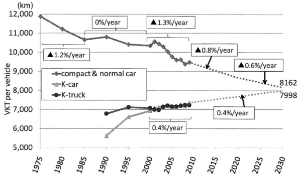
The VKT behavior has important effects on future fleet fuel use and GHG emissions. The trend of VKT per vehicle per year for each type of vehicle except for compact trucks is shown in Figure 11 (no data are available for compact trucks.) The historical VKT per vehicle data highlight several important trends. First, the trends are completely different for different vehicle categories. More specifically, though the VKT per vehicle for compact and normal passenger cars has been decreasing, that for K-cars and K-trucks has been increasing. Second, the VKT per vehicle for compact and normal passenger cars has been much larger than that for K-cars in any year before 2009.

(24)

(km) 12,000 12,000 _{0%/yea r} _AIL1.3%/year 11,000 10,000 A1.2%/yearA.8%/year - AO.6%/year

9,000 -compact& _{normal car}

> K-car -..- 8162 -8,000 ₈ _-e-K-truck .s "7998 7,000 _0.4%/year 6,000 0.4%/year 5,000 C 6? 0C) C2 10 )0 0

Figure 11. VKT per vehicle per year

[Transport Research and Statistics Office, MLIT, 2010]

The growth in VKT per vehicle for K-cars is 0.4% per year between 2000 and 2009. In addition, VKT per vehicle for K-trucks has a similar trend between 2000 and 2009. Therefore, the rate of growth in VKT per vehicle for K-cars and K-trucks is assumed to be 0.4% per year through 2030, taking into consideration historical VKT growth and government projections.

On the other hand, the growth in VKT per vehicle for compact and normal passenger cars is -1.2% per year between 1975 and 1985, 0% per year between 1985 and 2000, and -1.3% per year between 2000 and 2009. Therefore, the rate of growth in VKT per vehicle for compact and normal passenger cars is assumed to be -0.8% per year through 2020, and -0.6% per year between 2020 and 2030, taking into consideration historical VKT growth and government projections. In the present research, the rate of growth in VKT per vehicle for compact trucks is assumed to be the same as that of compact and normal passenger cars, because the growth trends of K-cars and K-trucks are similar. It is assumed that new compact and normal passenger cars are driven 12,700km in their first year, which is calculated based on the cumulative VKT per vehicle data in 2009 [Road Transport Bureau, MLIT, 2010]. After the first year, the VKT per vehicle

(25)

decreases at an annual rate (denoted r) of 6.5% for compact and normal passenger cars and 6.2% for K-cars as vehicles get older. This number is obtained by calculation using the least squares method. Thus, the VKT per vehicle of a vehicle aged i years is calculated as:

VKTi=VKTnewxe-"

Based on Figure 11 and this equation, the vehicle kilometers traveled by compact and normal passenger cars of different ages can be calculated. Figure 12 shows the annual distance traveled by the new compact and normal passenger cars at 5-year intervals between 1980 and 2005, and in 2009.

(km) 16,000 14,000 12,000 10,000 8,000 6,000 4,000 --- 1980 -1985 -1990 -1995 -2000 -.... 2005 2009 2,000 0 I 10 15 vehicle age 20 25 30

Figure 12. VKT per vehicle per year by model year (1980-2009)

In the same way, r is set to 0.062 (6.2%) for K-cars. Since no cumulative VKT per vehicle data for trucks is available, r=0.065 (6.5%) is used for compact trucks, and r=0.062 (6.2%) is used for K-trucks.

The total VKT for a given calendar year,

j,

is obtained using the following equation: VKTj= Zi Ni, j * VKTid

where Nij is the number of vehicles of age i in calendar yearj, and VKTid is the average annual vehicle travel for vehicles of age i in yearj.

(26)

2.2.5 Future Sales Mix Scenarios

Different scenarios are used to project the fuel use of light-duty vehicles under different market and policy conditions. These scenarios also allow us to understand the magnitude of technological and policy efforts that may be required to reduce fuel use of light-duty vehicle fleet.

A "future sales mix scenario" means the future sales share of new propulsion systems. In this research, Naturally-Aspirated Gasoline (Non-turbo Gasoline or Gasoline), Turbocharged Gasoline (turbo), Clean Diesel, Strong Gasoline Hybrid Electric Vehicle (HEV), Diesel Hybrid Electric Vehicle, Plug-in Hybrid Vehicle (PHEV), Battery Electric Vehicle (BEV), and Fuel Cell Vehicle (FCV) are taken into consideration as new propulsion systems in the future.

First of all, vehicles are divided into two types in order to build sales mix scenarios. The first type is called Standard Vehicles, which includes compact and normal passenger cars and compact trucks. The second type is called Light Vehicles, which includes K-cars and K-trucks. Then, four potential future sales mix scenarios were evaluated. (1) Government Scenario

In June 2008, the then Prime Minister, Yasuo Fukuda, talked about the government's vision that "An ambitious target to introduce Next Gen Vehicles (new propulsion technology vehicles such as hybrid vehicles and battery electric vehicles) at the ratio of half of the total new car sales should be realized by 2020." Since the sales share of the new propulsion vehicles was only 11.8% in 2010, this government scenario might be too optimistic. The details of the Government Scenario are shown in Table 6, Figure 13, and 14 [MOE, 2010]. Since the Japanese Government has projected the number of sales of each new propulsion vehicle, the percentage is obtained based on the total sales projections in the future.

(2) Half of Government Scenario

The sales percentages of new technology (all propulsion systems except for conventional gasoline vehicles) in each year in this scenario are the halves of those in the Government Scenario. This scenario has been created because the Government Scenario is too optimistic and it is desirable to have a less optimistic scenario based on the Government Scenario objectives. The details of the Half of Government Scenario are shown in Table 7, Figure 13, and 14 [MOE, 2010].

(27)

(3) Realistic Scenario

This is an original scenario and has been developed, based on some expert opinions and our own forecast, to provide a separately developed more realistic alternative to the optimistic Government Scenario. The details of the Realistic Scenario are shown in Table 8, Figure 13, and 14.

(4) No-change Scenario

This scenario assumes that the sales mix, such as the sales share of hybrid vehicles or electric vehicles, does not change in the future.

(28)

Table 6. Sales mix of the Government Scenario

[MOE, 2010; NGVPC, 2010]

Gov't (standard) Number of sales [thousands] %

2010 2020 2030 2010 2020 2030 Gasoline 81.96% 34.08% 15.94% Non-turbo (ICE) (81.96%) (34.08%) (15.94%) Turbo gasoline Diesel Clean diesel 4 186 134 0.13% 6.20% 4.66% Gasoline hybrid 17.90% 37.48% 34.03% Strong hybrid 550 1067 924 (17.90%) (35.58%) (32.12%) Mild hybrid 39 38 (0%) (1.30%) (1.32%) Micro hybrid 18 17 (0%) (0.60%) (0.59%) Diesel hybrid 76 81 0% 2.53% 2.82% Electricity PHEV 0.2 385 790 0.01% 12.84% 27.46% BEV 0 201 360 0% 6.7% 12.51% Hydrogen FCV 0 5 74 0% 0.17% 2.57%

Gov't (light) Number of sales [thousands] %

2010 2020 2030 2010 2020 2030 Gasoline 99.42% 74.98% 33.01% Non-turbo (ICE) (84.50%) (63.73%) (28.06%) Turbo gasoline2 _(14.91%) _(11.25%) _(4.95%) Electricity BEV 10 474 1244 0.58% 25.02% 66.99%

2 Since 41 models of K-cars/trucks (light vehicles) out of a total of 238 models of light vehicles were turbo gasoline vehicles (17.2%) [Road Transport Bureau, MLIT, 20101, turbo gasoline-using light vehicles are assumed to be 15% of all the gasoline vehicles for light vehicles.

(29)

Table 7. Sales mix of the Half of Government Scenario

Half of Gov't (standard) %

2010 2020 2030 Gasoline 82.10% 66.96% 58.00% Non-turbo (ICE) (82.10%) (66.96%) (58.00%) Turbo gasoline Diesel Clean diesel 0% 3.10% 2.30% Gasoline hybrid 17.90% 18.75% 17.00% Strong hybrid Mild hybrid Micro hybrid Diesel hybrid 0% 1.30% 1.41% Electricity PHEV 0% 6.40% 13.75% BEV 0% 3.40% 6.25% Hydrogen FCV 0% 0.09% 1.29%

Half of Gov't (light) %

2010 2020 2030 Gasoline 99.42% 87.50% 66.50% Non-turbo (ICE) (84.51%) (74.38%) (56.53%) Turbo gasoline (14.91%) (13.13%) (9.98%) Electricity BEV 0.58% 12.50% 33.50%

(30)

Table 8. Sales mix of the Realistic Scenario Realistic (standard) % 2010 2020 2030 Gasoline 82.1% 60.0% 35.0% Non-turbo (ICE) (82.1%) (57.0%) (31.5%) Turbo gasoline (3.0%) (3.5%) Diesel Clean diesel 0% 3.0% 5.0% Gasoline hybrid 17.9% 20.0% 28.0% Strong hybrid Mild hybrid Micro hybrid Diesel hybrid 0% 2.0% 2.0% Electricity PHEV 0% 10.0% 20.0% BEV 0% 5.0% 10.0% Hydrogen FCV 0% 0.0% 0.0% Realistic (light) % 2010 2020 2030 Gasoline 99.42% 90.00% 75.00% Non-turbo (ICE) (84.51%) (76.5%) (63.75%) Turbo gasoline (14.91%) (13.5%) (11.25%) Electricity BEV 0.58% 10.00% 25.00%

(31)

Sales mix (Gov't) 100% 90% 80% 70% 60% 50% 40% 30% 20% 10% 0% Z ICE E Turbo-SI

t Clean Diesel U HEV

U Diesel Hybrid PHEV EV N FCV

Figure 1

Sales mix (Gov't)

100% 90% 80% 60% 50% 40% 30% 20% 10% 0% = ICE 0 Turbo-SI -EV

Sales mix (Half of Gov't)

100% _!177,71 90% 80% 70% 60% 50% 40% 30% 20% 10% 0% m ICE U Turbo-SI

: Clean Diesel N HEV

M Diesel Hybrid PHEV EV * FCV

Sales mix (Realistic)

100% -80% 70% 60% 50% 40% 30% 20% 10% 0% SICE E Turbo-SI

Clean Diesel U HEV

N Diesel Hybrid PHEV

1 EV E FCV

3. Sales mix scenarios for standard vehicles

Sales mix (Half of Gov't)

100% 90% 70% 60% 50% 40% 30% 20% 10% 0%

=ICE

M Turbo-SI EV

Sales mix (Realistic)

100% 90% 80% 60% 50% 40% 30% 20% 10% 0% m ICE N Turbo-SI EV

Figure 14. Sales mix scenarios for light vehicles

From Figure 13, the Half of Government Scenario assumes the most modest change for standard vehicles among these three scenarios. On the other hand, the Realistic Scenario assumes the most modest change for light vehicles among these three scenarios because some experts doubt that battery electric vehicles will become popular so soon.

(32)

2.2.6 Vehicle Weight

Though Vehicle Fuel Consumption is a necessary input for the Fleet Model, it is not available for all vehicle categories such as K-cars or compact trucks. Therefore, that information is obtained in the present research by using the relationship between fuel consumption and vehicle weight.

2.2.6.1 Average Vehicle Weight for each vehicle category

Since average vehicle weight sold in a certain year is not available, weight distributions of in-use vehicles in 2008 are shown in Figure 15 [AIRIA, 2010]. There is no official vehicle weight data for K-cars and K-trucks. According to the catalog data, however, most of the vehicle weights of K-cars and K-trucks sold in 2010 were in the range between 700kg and 1,070kg [Road Transport Bureau of MLIT, 2010].

(mil) 18.0 16.0 14.0 12.0 10.0 -8.0 -6.0 -4.0 2.0 0.0 -5:' " compact truck

* compact passenger car

1 normal passenger car

- En

-c~O

N~O~

4r8 _2,

vehicle weight

Figure 15. In-Use Vehicle Weight Distribution in Japan in 2008 [AIRIA, 2010]

The approximate average weight of vehicle in each category is shown in Table 9. As for compact passenger cars, normal passenger cars, and compact trucks, the average weights are obtained based on the in-use vehicle weight distribution, using the median of each range. As for K-cars and K-trucks, the average vehicle weights are obtained by considering catalog data.

1

(33)

Table 9. Average vehicle weight for each vehicle category Average Weight Data Source

Compact truck 1625 [kg] in-use vehicle weight distribution, 2008 Compact passenger car 1187 [kg] in-use vehicle weight distribution, 2008 Normal passenger car 1573 [kg] in-use vehicle weight distribution, 2008

K-car/ K-truck 850 [kg] new vehicle catalog, 2010

2.2.6.2 Relationship between Fuel Consumption and Vehicle Weight

A precise relationship between vehicle weight and vehicle fuel consumption for light-duty vehicles in the United States has been identified [Cheah, 2010]. In the U.S. case, the adjusted, combined city/highway (55/45) fuel consumption and curb weight of all model year 2006-2008 light-duty vehicles offered in the U.S. revealed a general positive correlation.

Figure 16 plots the fuel consumption (L/lOOkm) of new passenger vehicles (compact and normal passenger cars and K-cars) that were sold in 2008, measured by JC08 mode (Japanese test cycle) [Road Transport Bureau of MLIT, 2010]. There are 225 samples in the plots. As expected, a positive correlation was found for passenger cars sold in Japan. Based on the data, formulas for fuel consumption and vehicle weight (curb weight) were obtained as shown in Figure 16. The linear correlations, which are shown in Figure 16, are as follows:

(1): y = 0.0066x - 0.6618 (AT, MT) (2): y = 0.0047x + 0.6267 (CVT) (3): y = 0.004x - 1.4279 (HEV)

(34)

(L/lOOkm)

22.5

20 *T

MT

17.5 - AT -- (1)

--.0

15 -- ACVT

-E 12.5

0 Hybrid-

-

-(2

103 U

S7.5___

5

-2.5

vehicleweight

(kg)

Figure 16. Fuel Consumption and Vehicle Weight by JC08 mode in Japan [Road Transport Bureau of MLIT, 2010]

Since most of the vehicles in Japan are AT (Automatic Transmission), the formula for AT and MT (Manual Transmission) is going to be used to calculate the fuel consumption by using the vehicle weight.

2.2.7 Vehicle Fuel Consumption

2.2.7.1 Historical Data of Vehicle Fuel Consumption for all passenger cars

It is very difficult to get consistent data for vehicle fuel consumption because there are two test cycles for measuring vehicle fuel economy. The first one is called the 10-15 mode cycle, which has been used for emission certification and fuel economy for light-duty vehicles. Emissions are expressed in g/km [JISHA, 1983]. The second one is called JC08 mode. This new JC08 chassis dynamometer test cycle for light vehicles (< 3,500kg GVW) was introduced when Japan's 2005 emission regulation was established. The test represents driving in congested city traffic, including idling periods and frequently alternating acceleration and deceleration [MLIT, 2006]. Measurement is made twice, with a cold start and with a warm start. The test is used for emission measurement and fuel economy determination, for gasoline and diesel vehicles. The

(35)

JC08 test will be fully phased in by October 2011. The driving schedules for both test cycles are shown in Figure 17 [MLIT, 2006]. The on-road fuel consumption is higher than the test values because of differences between actual driving conditions and trip patterns, and the test cycles, as well as the less than ideal state of maintenance of vehicles and aggressive driving behavior [Hellman and Murrell, 1982]. However, fuel consumption by test cycles is regarded as on-road fuel consumption in the present research.

(36)

Cold st

11mo 100 - 80 E 60 > 40 U 20 0 Time (s) JC08C mode 100 t80 E o -S20 1) 0 > 0 200 400 600 800 1000 1200 Time (s)

0

100 200 300 400 500 art

de

-Ave.speed 30.6km/h -Maxspeed 60km/h -duration 505 sec -Ave. speed 24.4km/h -Maxspeed 81.6km/h -duration 1,204 sec

Figure 17. Japanese test cycles for measuring vehicle fuel economy [MLIT, 2006]

Figure 18 shows the new passenger car vehicle fuel consumption trend from 1993 to 2009 [Road Transport Bureau of MLIT, 2010; JAMA, 2010]. Vehicle fuel consumption

-- rip

Hot startl

10:15 mode

100 -Ave.

speed

r80 22.7km/h E -Maxspeed 40 70km/h 20 AM-duration- m o 0 0 100 200 300 400 500 60 660 sec Time (s) JCO8H mode 100 -Ave. speed S80 -24.4km/h -Max speed

81.6km/h

_ 20 -duration > 0 200 400 600 800 1000 1200 1,204 sec Time (s)

(37)

in 2009 is obtained from JAMA's fuel consumption trend because the data has not yet become available from MLIT. Since the MLIT fuel consumption values are about 0.5[km/L] higher than JAMA reported fuel consumption values, the change of fuel consumption from 2008 to 2009 in JAMA's data was used in order to get tentative MLIT data for 2009. In addition, the historical data for fuel consumption is measured by

10-15 mode and converted to JC08 mode by the following formula [JSAE, 2007]:

FC by JC08 [km/L] = FC by 10-15 [km/L] * 0.913

Based on the Kyoto protocols, the Energy Conservation Law was revised in 1998 and it introduced Top-Runner Target Product Standards. The fuel economy targets were based on weight classes, and required 22.8% improvement over the 1995 weight class averages by the year 2010. The fuel economy target for passenger vehicles in 2015 is 16.8krn/L (5.95L/lOOkm), measured by JC08 mode. Since the fuel economy target is determined based on the vehicle weight range, this fuel economy is the average for passenger vehicles. Here, the vehicle weight distribution is assumed to be constant in

the future. (L/lOOkm) 9.5 9 0- 8.5 Q. _iL E 8

7.5

5

6.5 9 6 CU > ₅

4.5

1

1990 1995 2000 2005 2010 2015 2020 2025 2030

Figure 18. The trend of vehicle fuel consumption for all passenger vehicles [Road Transport Bureau of MLIT, 2010; JAMA, 2010]

2.2.7.2 Vehicle Fuel Consumption for each vehicle category of Model Year 2008 In Table 9, the average vehicle weight is obtained, though the source is different from

(38)

one category to another. From this section, the average vehicle shown in Table 9 is regarded as vehicle weight sold in 2008 (Model Year 2008). From both Figure 16 (which shows the relationship between vehicle weight and fuel consumption) and Table 9 (which shows average vehicle weight for each vehicle category), vehicle fuel consumption for each vehicle category of Model Year 2008 is obtained, as shown in Table 10.

Table 10. Vehicle fuel consumption for each vehicle category of Model Year 2008

Average Weight Vehicle Fuel Consumption (JC08 mode)

Compact truck 1625 [kg] 10.06 [L/lOOkm]

Compact passenger car 1187 [kg] 7.17 [L/lOOkm]

Normal passenger car 1573 [kg] 9.72 [L/lOOkm]

K-car/ K-truck 850 [kg] 4.95 [L/lOOkm]

2.2.7.3 The trend of Vehicle Fuel Consumption

for

each vehicle category

In section 2.2.7.1, historical vehicle fuel consumption for all passenger cars, including compact and normal passenger cars, and K-cars, was obtained. From this data, the trends of how fuel economy has been improved can be seen. Based on the historical trends and vehicle fuel consumption in 2008, vehicle fuel consumption for each vehicle category is calculated and shown in Figure 19. Specifically, the historical percentage changes of fuel consumption for all passenger cars were used for the calculation.

(L/lOOkm) 14 13 c 12 0 S11 E 10 91 _{-+-compacttrucks}

8

8 _{-a-normal passenger cars}

7~ _x

12 6' x+compact passenger cars

- - K-cars/trucks _0 5 0.5%/year 4 A1-A30o%/year A2.%/year7.17[L/1km](1,187.3kg) 3 1 14.95[L/10km] (850kg) 1990 1995 2000 2005 2010

(39)

In the fleet model, fuel consumption is assumed to be constant before 1993 because no data is available. Although the trend of vehicle fuel consumption cannot be the same for all vehicle categories, especially because historical vehicle weight change is quite different from one vehicle category to another, the trends of vehicle fuel consumption for each vehicle category are assumed to be the same as that for all categories of passenger cars.

2.2.7.4 Future Reductions in Fuel Consumption

There are several technologies and approaches to improve vehicle fuel consumption. They include improvements in the engine and transmission and use of alternative propulsion systems such as hybrid vehicles. In this section, the following two approaches are explained.

The fuel consumption trend that is realized in practice will depend on the degree of emphasis placed on reducing fuel consumption, because fuel consumption reductions can be offset by the negative impacts of increasing vehicle size, weight, and power. For the purpose of understanding the influence of the trade-off of the performance, size, and fuel consumption, the concept of Emphasis on Reducing Fuel Consumption (ERFC), which is shown in Equation 2, is helpful. [Heywood, 2010]

Fuel Consumption (FC) Reduction Realized on Road ERFC =(2

FC Reduction Possible with Constant Performance and Size

ERFC measures the degree to which improvements in technology are being directed toward reducing onboard fuel consumption.

Since fuel consumption reduction is realized not only by the improvement of mainstream gasoline vehicles, but also by the prevalence of new propulsion systems such as hybrid vehicles and battery electric vehicles, it is necessary to consider future reductions in vehicle fuel consumption for different propulsion systems. The relative fuel consumptions of different propulsion systems are shown in Figure 20 [MOE, 2010]. In the years between 2010 and 2020, or 2020 and 2030, the relative fuel consumption is assumed to change linearly. Technical progress in internal combustion engines has historically been roughly linear and relatively well-behaved [Chon and Heywood, 2000;

(40)

Heywood and Welling, 2009], which supports the linear assumption going forward. 1.2 1.6 3.80 0 48462 0.27 0.6 0.0 2010 2020 2030

U Gasoline

=Turbo

-,Diesel 2 Strong Hybrid Diesel Hybrid E PHEV BEV

Figure 20. Relative fuel consumption for different propulsion systems [MOE, 2010]

These Japanese Government fuel consumption numbers for 2030 correspond to numbers for 2030 calculated for the U.S. or EU when the ERFC is about 50%. Comparing the relative fuel consumption of US/EU and Japan, there are two major differences.

(1) The mainstream gasoline engine of Japan does not improve as much as that of the US and EU.

This is because vehicle fuel consumption in Japan is already lower than that in the US and EU. Therefore, the potential reduction in fuel consumption is not so large in Japan.

(2) The relative fuel consumption for strong gasoline hybrid is smaller than that for diesel hybrid in Japan, though it is the opposite in the US and EU.

Strong Hybrid is most effective in the following conditions: 1) repeated acceleration and running at a low speed, and 2) light vehicle weight. Since both the JC08 test cycle, which represents driving in congested city traffic, and Japanese small vehicle size suit these conditions, a strong hybrid system can achieve lower fuel consumption in Japan successfully.

(41)

2.3 Model Calibration

Before the fleet model is used to simulate future fuel use and GHG emissions, it must first be calibrated using historical data. This will help ensure that the characteristics of the current fleet contained in the model correspond closely to the actual on-road fleet in Japan. The model calibration can be seen in the following chapter.

(42)

3. NEARER-TERM FLEET FUEL USE AND GHG TRENDS (through 2030)

3.1 Vehicle Stock

Before comparing future projections of light-duty fleet characteristics, the model results are first evaluated against historical trends. Figure 21 shows the model calculated vehicle stock compared with data by the Automobile Inspection and Registration Information Association [AIRIA, 2010]. The number of vehicles in the Japanese light-duty vehicle fleet increased from about 65.3 million vehicles in 1997 to about 71.4 million vehicles in 2006. Then, it decreased to 71.0 million vehicles in 2009. The increase in stock came from the light vehicles, especially K-cars. However, the total numbers in the light-duty vehicle fleet started slightly decreasing from 2007 because the number of standard vehicles has been decreasing rapidly. In Figure 21, the model results are very close to the historical fleet data. Detailed data for each vehicle category is shown in Figure 22.

(mil)

75

f69-6 65

55

45

35

25 ll LDVs

_{Gov'tforecast: 67.2}

standard

40.1

Govt

forecast:38.1

2s.9

.---Gov't forecast:

29. -

Fleet Data (all LDVs)

---

Fleet Model (all LDVs)

-

Fleet Data (standard)

---

Fleet Model (standard)

-

Fleet Data (light)

---

Fleet Model (light)

Figure 21. Vehicle stock (fleet model results compared with historical data) [AIRIA, 2010; MOE, 2010]

(43)

(Mil) Vehicle stock (compact & normal cars) 45 43 -fleet data -41 -- fleet model -39 - - -37 35 1995 2000 2005 2010 2015 2020 2025 2030 (mil) Vehicle stock (compact trucks)

7 6 - - -- fleetdata 5 --- fleet model 3 2 -1995 2000 2005 2 2 2---2010 2015 2020 2025 2030

25 Vehicle stock (K-cars)

20 -

-15

1 -- fleet data

--- fleet model

1995 2000 2005 2010 2015 2020 2025 2030

(mil Vehicle stocks (K-trucks)

12

-flee data --- fleet model

1995 2000 2005 2010 2015 2020 2025 2030 Figure 22. Vehicle stock for each vehicle category

(Fleet model results compared with historical data)

[AIRIA, 2010]

Table 11I shows the average error in the light-duty vehicle stock since 1997 relative to the AIRIA data. The error between data and model is less than 0.3% in any time period, which means this fleet model forecasts the number of light-duty vehicles correctly if the future assumptions of inputs are correct.

Table 11. Difference between fleet data and model calculation Period Difference in light-duty vehicle stock [%]

1997-2000 0.30%

2001-2005 -0.02%

2006-2009 -0.04%

There are several reasons for the decrease or increase of vehicle stock of each category.

The reasons for the decrease of the compact and normal passenger car stock from 2005 are as follows:

(44)

2. The number of people who purchase passenger cars for the first time has been decreasing because passenger cars have long been widely owned in Japan. In other words, when new cars are sold, old cars are scrapped, in most cases. 3. The increase of driver's license holders (80 million in 2009) has been much

slower. This is because of the decreasing population, in particular the decrease of the population of younger generations.

<K- cars>

In contrast to the compact and normal passenger cars, the K-car stock has still been increasing because the new K-car sales have not dropped rapidly yet. The reasons for the increase of new K- car stock from 2005 are as follows:

1. Due to the high gasoline price, some drivers prefer K-cars to compact and normal cars. Drivers can save money on gasoline because fuel economy for K-cars is better than that for compact and normal passenger cars.

2. Taxes for K-cars, such as vehicle weight tax, vehicle tax, and vehicle acquisition tax, are lower than those for compact and normal passenger cars. Details on taxes are shown in Table 12 [Road Transport Bureau, MLIT, 2011; NAVI, 2011; TMG, 2008].

However, the global recession slowed the increase of the K-car stock. Table 12. Taxes for passenger cars in Japan

[Road Transport Bureau, MLIT, 2011; NAVI, 2011; TMG, 2008]

Payment time K-cars Compact & normal passenger cars

Vehicle acquisition when purchased 3% of the car 5% of the car price

tax price

Vehicle weight tax every 2 years JPY 7,600 JPY 10,000-60,000

(Depending on vehicle weight)

Vehicle tax every year JPY 7,200 JPY 29,500~111,000

(Depending on displacement)

The reasons for the decrease of compact truck stock are as follows: 1. Recession and high gasoline price

2. In the Japanese logistic system, more efficient freight transport has been achieved. Logistic companies have gradually come to choose larger trucks rather

Assessing the fuel Use and greenhouse gas emissions of future light-duty vehicles in Japan