FLIGHT TRANSPORTATION LABORATORY
REPORT R78-1
THE ASNA FORMULA:
A NEW CONCEPT
COST PER PASSENGER MILE
(KILOMETER)
* A
Asad Nasr
General Manager
Middle East Airlines
0L bi l March 1978
T H E A S N A F 0 R M U L A
A N E W C 0 N C E P T
C 0 ST .J PF E R PASSFWtER M IL E (K ILONME TE R)
Asad Nasr, General Manager of Middle East Airlines
Flight Transportation Laboratory Massachusetts Institute of Technology
77 Massachusetts Avenue Room 33-412
Cambridge, MA 02139 FTL Report R78-1
March 1978
Preface
In May 1977, we were honored to have Mr. Asad Nasr, Chairman and President of Middle East Airlines give a Flight Transportation Seminar at MIT on the ASNA formula. in view of the interest generated, and a need for wider discrimination amongst aviation planners and managers, it was mutually decided that a report authored by Mr. Nasr would be published by the Flight Transportation Laboratory. We are happy to collaborate in this joint venture, since it should lead to better analysis.of various problems in airline planning.
Robert W. Simpson Director, FTL
Mr. Asad Yusuf Nasr
Chairman and President, Middle East Airlines (MEA) Beirut, Lebanon
Mr. Nasr was a graduate of Cambridge University in Mathematics and Law in 1950, and received his MA in 1955. He has taught Mathematics and Statistics at the American University of Beirut before joining MEA in 1955 as General Planning and Economics Manager. He developed the ASNAFormula for Aircraft and Schedule Evaluation in 1970 and has been
the author of several articles on Air Transport and Management Systems.
He received the 1st Annual Airline Technical Management Award from Air Transport World in 1975. He has received various honors including Commander of National Order of Tchad, Officer of the National Order of Lebanon, Order of the Republic of Egypt, the Laborer Medal of Lebanon,
LIST OF CONTENTS
1D.
PAGE
An Economic Overview
Introduction to the Problem
51-Fields of Application 15
A- Change of Aircraft Configuration 15
B- Choice Between Types of Aircraft 18
C- Bilateral Negotiations 28
D- Aircraft-Mile Costs Vs Seat-Mile Costs 29
E- Range/Payload Substitution 3D
F- Aircraft Design Modification 32
G- Determination of Air Fares 33
H- Deployment of Different Fleets 38
The Search for a Solution 40
Statement of Inputs 42
Input Form 43
Explanations & Definitions 45
Sector S 45
Base Period P 49
Data 58
(i)
Statement of Outputs Illustration I Summary of Results-I Graphic Presentation I Illustration II Summary of Results-II Applications A.1 A.2 A.3 A.4 A.5 A.6 A.7 A.8 A.9 Appendix I - Illustration I Appendix II - Illustration II (ii) 104
THE ASNA FORMULA
AN ECONOMIC OVERVIEW
Demand and Revenue
The demand for air transport is affected by the usual
extraneous factors, demographic, social and economic, as well
as those falling properly within the sphere of the industry itself such as the quality of service, safety, .reliability, punctuality, speed, frequency comfort, price.
But whatever the overall volume of the demand thus
determined, it will not be evenly distributed. There will
always be fluctuations in the demand for the individual
fliohts.
This emphasis on the individual flight is simply a
reflection of the nature of scheduled air transport and of the indivisibility of the air transport vehicle. Obviously,
the use of averages would reduce the magnitude of demand
fluctuations and would therefore make any analysis
The fluctuations in individual flight demand have wide ranging effects on several aspects of the Air Transporti Industry such as scheduling, optimum size of aircraft, frequency and capacity, price elasticity and the determination of fares, etc.
It will thus be observed that airlines tend to offer a level of capacity falling between the extreme values of demand, high and low. They almost never choose to operate an aircraft vwith a capacity sufficient to satisfy the demand for each
and every flight. Equally, they are most unlikely to operate, continuously, on the basis of a virtually full aircraft.
In the first case, i.e. if the airline were to operate an aircraft sufficiently large as to cater for the highest demand levels, then it would be offering excessive capacity on most remaining flights. This would mean lower average load factors and lower profitability. Such consequences are not only harmful to the airline itself but, also, to the public, as lower load factors and lower profitability will necessarily mean that fares will be maintained at a higher level than would have been possible otherwise.
-3-,7
In the second case, i.e. where the airline is aiming at a continuous operation with a very high load factor, (say above 90%),
there will be very few flights in respect of which the demand is
totally satisfied by the capacity offered. On all the remaining
flights, and they are the vast majority, there will be more
passengers than seats, which means that certain numbers of
passengers will be turned away, i.e. there will be frequent
flights with overflows, some of substantial proportions. These
will cause public dissatisfaction and outcry of such intensity
as to harm the development of the industry and, probably, bring
3
about the intervention of regulatory authorities.Furthermore, the airline would not be maximizing its
profits, since, at such load factors, as will be shown later,
total profits can be increased by operating an aircraft with a
greater seating capacity.
Airline managements are therefore required to determine
that level of capacity which, given the specific volume and
fluctuations of demand on a particular route or segment,
Another consequence of the fluctuations in the demand for individual flights relates to price elasticity and the determination of fares. On the basis that the demand for air transport is price elastic, the increase in demand, resulting from a given reduction in price, cannot be fully satisfied by the airline because of the fluctuations in
individual flight.demand. Also, the airline itself cannot achieve the full increase in revenue indicated by the price elasticity.
Cost
There is a positive correlation between aircraft size and aircraft/mile* costs, and a. negative correlation between aircraft size and seat/mile* costs.
Airlines are constantly attempting to strike the right balance between the advantages of the lower seat/mile* costs of the larger aircraft against the advantages of the lower aircraft/mile* costs of the smaller aircraft. On the one hand,
I-.
escalation in costs, public clamour for lower fares, conservation
of energy, protection of the environment, etc, are constant
pressures on the airlines to aim at lower seat/mile* costs,
mainly by utilizing larger aircraft. Conversely, their own
economic survival requires that they utilize an aircraft of a
limited capacity and, consequently, of lower aircraft/mile*
costs, with which they can achieye profitable (higher) load
factors.
In other words whenever an airline considers the acqvisition
of a new type of aircraft, or the deployment of an existihg type on a certain route or segment, it immediately faces this conflict
between the advantages, in lower seat/mile*costs, of the larger
aircraft, as against the advantages, in lower aircraft/mile* costs,
of the smaller aircraft.
A New Concept: COST PER PASSENGER/MILE*
It is suggested that this conflict can be reconciled by
adopting a new concept of passenaer/mile* cost. In principle,
and provided there are no overriding outside constraints,
airlines should decide in favour of operating the aircraft/
frequencies/schedule combination which results in the lowest
passenger mile* costs.
The evaluation of the passenger/mile* cost requires a procedure for the conversion of seats into passengers. This would make it possible to calculate the passenger/mile* cost from the traditional seat/mile* or aircraft/mile* cost.
The conversion factor (seats into passengers) is obviously a function of the particular market conditions: the total volume of demand and the prattern of its fluctuations over individual flights, existing schedules by all carriers, frequencies and types of aircraft.
THE ASNA FORMULA
The ASNA formula provides such a function. It defines the conversion factor in terms of the various market and operating factors enumerated above.
Consequently, the ASNA Formula can be utilized to measure Marainal Seat Utilization, MSU(a), and Marginal Acceptance, MA(b)
* or kilometer
(a) MSU = The increase in the passenger load due to one additional seat on the aircraft
(b) MA = The percentage increase in the passengers accepted on an aircraft due to l increase in demand
It will be readily seen that these tools simplify, radically, the task involved in decision making in several
fundamental areas in the field of air transport. The following are some important examples:
1. Airline decisions regarding the selection of aircraft,
scheduling and deployment of fleets: The relationship
between the Marginal Operating Cost - MC, the MSU, and the MA, determines the optimum aircraft and the optimum
schedule for maximum profits.
2. The pricing of air transport: The relatioanship between
the price elasticity, usually between -1.5 and -2.0,
and the MA determines the price and the load factor
for maximum profits.
3. From the MSU, the Marginal Traffic, MT(c), can be
measured. Most passengers travel on a return basis, and-thus a factor f can be established equal to the
ratio of MT to MSU. f is usually between 1.3 and 1.6.
(c) MT = The increase in all passengers carried (total passenger
traffic on the system) due to one additional seat on the
aircraft
4. The assessment of public dissatisfaction related to
inability to find s-eats on the chosen flights (overflows)
A distinctive feature of the ASNA formula is that it is
both a macro and a micro econometric model.
Introduction to the Problem
The selection of an aircraft most suited for an airline's
network and traffic is, without doubt, the most important decision it takes, entailing far reaching consequences which touch almost
every function and activity and which span two decades or more
of the airline's future.
In order to make such a selection, the airline carries
out an assessment of all possible alternative aircraft that are
available on the market (old as well as new).
Broadly speaking, the assessment covers the following areas:
1. Specifications and Performance of the various aircraft
with a view to determining their suitability to the
-
9
-and any additions to that network planned for the future. Any operational limitations or constraints
are identified and quantified, particularly on
payloads. In addition, flight times and fuel
consumption are determined.
2. The operating costs of the various aircraft. There are obviously numerous difficulties associated with this area
of investigation but there are generally agreed procedures
which most airlines follow in making such assessments,
and experience has shown that they are sufficiently
accurate for the purposes for which they are intended.
These costs include the aircraft standing charges such
as depreciation, interest, insurance etc... cockpit
and cabin crew costs, other fixed costs and all variable
operating costs. Flight times and fuel consumption
figures, determined under item one above, from the basis
for these estimates.
3. The revenue expected to be earned by the aircraft on the
various routes and segments of the defined network. As
will be shown herebelow, this item
poses
many serious difficulties, specifically, in estimating the passengersObviously the final decision would be in favour of the
aircraft which shows the highest difference in revenue as per
item three above over cost as per item two above.
Any limitations imposed by item one above would either
result in lowering revenue as in the case where the permissible
load is reduced, or would result in increasing cost as in the case of a requirement for an extra landing en route. Both are therefore reflected in the difference between revenue and cost.
REASONS FOR VARIATION IN PASSENGER LOADS
For the same market, schedule and airline, one aircraft
can show higher passenger loads than another for one or both
of the following elements:
1. Greater passenger appeal associated with speed, range
(non-stop capability), spaciousness, improved passenger amenities, reliability, safety record, etc...
2. Greater seating capacity enabling it to carry more
- 11
-The first of these elements is mostly of a subjective nature and can best be assessed through analysis, observation and opinion
surveys. But even when this is done, and some passenger preference factor is established, it would still be difficult to determine the
exact amount of revenue that can be earned in consequence because
it
would obviously depend on the capacity
of the aircraft and would therefore be related to the second element above.As to the second element, the problem is one of converting seats into passengers, and the two are never the same as long as
capacity is a constant while demand is variable, nor can they be
related by a fixed ratio as long as conditions in any two given
markets are never identically the same.
To illustrate, assuming we are comparing two aircraft,
Aircraft A with 150 seats and an hourly cost of $3,200 and
Aircraft B with 160 seats and an hourly cost of $3,300. The
comparison resolves itself into determining whether the ten
extra seats available on Aircraft B would result in carrying a
sufficient number of additional passengers to pay for the 100
Dollars extra cost per flying hour and leave a surplus. If the
answer to this question is positive then, other things being
equal, the choice would certainly be in favour of Aircraft B
as against Aircraft A.
But how does one determine the answer to such a question?
Obviously there are flights which operate completely full and on
which the airline is
obliged to turn away passengers who would have
wished to travel on the particular flight. The problem in
such a
case would be to determine the number of passengers thus turned
away. One-? or Two-? or three etc up to the maximum of ten extra
available seats.
In
the search for a solution, it
has first suggested that this
question can best be answered by the Reservations Department. They
would know how many passengers were placed on the "waiting list".
But
upon reflection it
was clear that this could not be the case. In
the first place, not all passengers accept to be placed on the waiting
list. Also, many passengers wishing to travel do not contact the
airline at all. They call their travel agent for their booking, and
the travel agent would in
turn contact the airline and obtain a
negative response without having first announced the name of the
passenger. In
such a case the airline would have no record whatsoever
of the turned away passenger or passengers. Equally, once the agent
gets a negative response for a particular flight, he would not contact
the airline again in
respect of another passenger.
But even if
it
were possible to overcome these difficulties by
setting up some system of recording all such unsatisfied requests,
13
-another problem arises, namely that all such information relates to the past while what is required is an assessment of a dynamic future.
What is needed is to identify the cases where such overflows would
take place in future years and the number of passengers that would
be turned away in each such case, and it is evident that the obvious
solution of taking each flight of the base year and increasing
the number of passengers actually carried on it by the assumed per-centage growth would not yield anything of value as the distribution
of passengers over the days and the flights is affected by random factors.
Furthermore, on some flights the number of passengers actually
recorded is not the number of those whose first choice was that particular flight. As long as there are flights which turned-away- passengers there are others which received such passengers and which consequently show a
larger number of passengers than they would have if all passengers could
be accommodated on their flight of first choice. There are also the
effects of "No-shows", ship-side sales, etc...
Again the flights of an airline do not remain exactly the same
from year to year and it would therefore be difficult to treat them in
the manner suggested whereby each flight would be treated individually.
Above all it must be remembered that on any given route there are
carried by one airline may be passengers whose first choice was another airline and who only travelled on the particular airline when they failed to get seats on the airline of their first choice.
When these questions were first encountered, the immediate and
obvious reaction was to contact other airlines of greater experience. in aircraft selection and find out what methods they had developed over the years.
Approaches were made to several such airlines. Their response came as a complete surprise. They all declared that they had no such formula and that the only way to deal with this particular problem was to use judgement based on experience.
At first the suspicion arose that it was only a matter of the airlines not wishing to give out something they had worked hard to develop and which, they considered, gave them a valuable tool which they would be ill advised to make freely available to others.
It was therefore decided to approach the manufacturers them-selves who, it was presumed, because of the magnitude of their interest, would have developed a complete arsenal of such weapons. But they also gave the same disappointing answer, namely, that they were not aware of any such formulae and that, in effect, they
- 15
-lend itself to a scientific approach and could only be handled by judgement.
Other attempts were made by calling on the assistance of some
leading aviation consultants. Their response were similar.
One of the manufacturers suggested that a possible solution,
which he applied in
such cases, was to take the six or seven peak
weeks and assume that fifty percent of the extra seats available
will
abe
utilized and that the next fullest six or seven weeks will
mean
utilizing a quarter of the extra seats available.
Evidently
such a solution is
totally arbitrary, and it
completely ignores all
the other relevant variables such as the number of the extra seats
or the load factor achieved on the particular route, or the seasonal
and directional variations, etc...
In
the following paragraphs, specific examples are given to
illustrate the wide range of executive decisions which, in
the final
analysis, can only be resolved by the conversion of seats into passengers.
Fields of Application
A- A decision is
required on a proposal to enlarge the galley on one
type of aircraft in
order to offer a better service to its passengers at the
cost of the loss of four seats on that aircraft. Obviously, no such decision
can be properly taken without first assessing the finanacial loss which would
result from the loss of the four seats. It is also obvious that the loss
will not be equal to the revenue from four passengers on all the flights operated with the type of aircraft under consideration.
In other words, assuming that the average revenue per passenger per flying hour is 50 Dollars and assuming the aircraft has, a dalily utilization of ten hours, it cannot be assumed that the loss of the four seats will mean the loss of 4 times 50 Dollars times 10 hours i.e. 2000
Dollars per aircraft per day. This is due to the fact that not all the flights are full and that on those flights which carry less than a full complement of passengers, one or more of the lost seats will not actually mean loss of revenue. Thus we can only say at this stage
that the loss of revenue resulting from the loss of the four seats is less than 2000 Dollars.
We can also say without further investigation that there will be some loss due to the loss of the four seats. Unless the airline is operating in a most uneconomical manner, there are bound to be certain days and certain hours when the demand will reach a level at which the missing four.seats will be translated into loss of passengers and there-fore into loss of revenue.
- 17
-Thus we can say that the loss due to the elimination of four seats
is somewhere between 0 and 2000 Dollars per aircraft per day.
Evidently this is too wide a margin. If it should prove to be only
20 Dollars, say, there would be no argument about enlarging the galley,
because it can be safely assumed that as a result of the improved service
to the passengers there will be at least one extra passenger per day who
will fly with this airline for a half hour sector because of the
attraction of the improved passenger service. The revenue from such
an additional passenger on a half hour sector would amount to 25 Dollars
and would therefore more than comensate for the loss of the four seats.
On the other hand, should the loss of revenue prove to be of the
order of $ 1000 per aircraft per day, then the improved galley must attract
two extra passengers on every flight, and as some flights will be full, the
remaining flights must attract proportionately more than two extra passengers to compensate.
It is essential therefore to determine, with reasonable exactitude, the loss of revenue associated with the loss of seats.
B- A decision is required on a choice between the DC8-62 and the DC8-50
aircraft. The first aircraft has thirty more seats but costs two million
Dollars more to purchase. Its hourly cost is $ 420 higher, including the
higher depreciation, interest, and insurance resulting from the higher
initial price.
The two aircraft would therefore compare in the following manner:
Table II
DC8-62
Seats Available
Hourly Costs (Dollars)
180
3420
DC8-50
150 3000
- 19
-B.1- To compare the two aircraft on the basis of equal frequency, say, five per week or per day for each of the two aircraft, and determine whether the larger aircraft can earn sufficient revenue with the 30 extra seats to pay for the additional cost of $ 420 per flight per hour.
or, alternatively,
B.2- To compare the two aircraft on the basis of equal capacity, say, 900 seats per day or per week, which would mean operating five flights with the larger aircraft against six with the smaller; and determine whether the saving in cost of $ 900, representing the difference between six one hour flights at $ 3000 and five one hour flights at $ 3420, would not be more
than wiped out by the loss of revenue due to the loss of one frequency by the larger aircraft.
It should be emphasized in respect of these two comparisons that the answers required should cover not only one year but the whole operating life envisaged for the particular aircraft.
It can be readily seen that, assuming that the two aircraft are operated with equal frequency, the smaller aircraft is more likely to show better results during the first year or two because it is unlikely
that demand will exceed its capacity on too many occasions. But as
traffic grows, in the normal course of events, these occasions will become more and more numerous and the capacity of the larger aircraft will come into higher and more frequent use.
Furthermore it will be noted that increasing the frequency of operation with the smaller aircraft, whenever necessary, will produce a smaller percentage increase in capacity and would therefore result in a smaller drop in load factors. The following table illustrates this point:
- 21 -TABLE III AIRCRAFT A FREQ SEATS L.F. 6 6 .6 7 8 9 10 11 13 14 16 18 20 23 26 29 900 900 900 1050 1200 1350 1500 1650 1950 2100 2400 2700 3000 3450 3900 4350 AIRCRAFT B FREQ SEATS L.F. 900 900 900 1080 1260 1440 1440 1620 1980 2160 2340 2700 3060 3420 3960 4500 YEAR TRAFFIC 450 509 575 649 734 829 937 1059 1196 1352 1528 1726 1951 2204 2491 2814 EQUAL EQUAL EQUAL LOWER LOWER LOWER HIGHER HIGHER LOWER LOWER HIGHER EQUAL LOWER HIGHER LOWER LOWER
Assumptions
1- Frequency will be increased whenever load factor exceeds 65 percent.
2- Traffic will increase annually by 13 percent.
From the above table it can be seen that of the sixteen years for which the calculations have been made, representing the generally acceptable life of an aircraft,
- 4 years showed equal load factors
- 8 years showed lower load factors for the larger aircraft
- 4 years showed higher load factors for the larger aircraft
Furthermore, the smaller aircraft means a higher frequency and this is always beneficial in terms of attracting passengers and stimulating traffic.
Against these advantages in favour of smaller aircraft it should be remembered that larger aircraft have the advantage of a lower break-even load factor and it is therefore necessary to compare quantitatively the
- 23
-two elements in order to arrive at a net result.
In the specific example we have been examining, it will be seen that the comparison on the basis of equal frequency, as suggested in the
first alternative, can be reduced to the specific question of determining the difference between the average passengers on the five flights of the larger aircraft and the average on those of the smaller aircraft.
We have already seen that the difference in hourly costs is $ 420
which is the difference between $ 3420 and $ 3000. This means 8.4
additional passengers per flight on the basis of a revenue rate of $ 50
per passenger per hour, i.e., a matter of whether the thirty extra seats
available on the larger aircraft will mean an extra load of 8.4 passengers
on the average flight.
Similarly, in considering the second alternative of equal capacity,
we have already determined that the difference in total cost of all flights
is $ 900, and as we have been assuming an hourly passenger revenue rate.of
on its six flights 18 passengers more than what the larger aircraft will
carry on its five flights.
The answers to these questions would obviously depend, very largely, on the following two factors:
1. The load factors at which Airline X and the other airlines are operating: the higher the load factor, the more efficient the larger aircraft.
2. The variance of the load factor: again, the higher the variance,
the more efficient the larger aircraft.
The validity of statement under 1. above is fairly obvious and
does not require further comment. The second statement, however, is
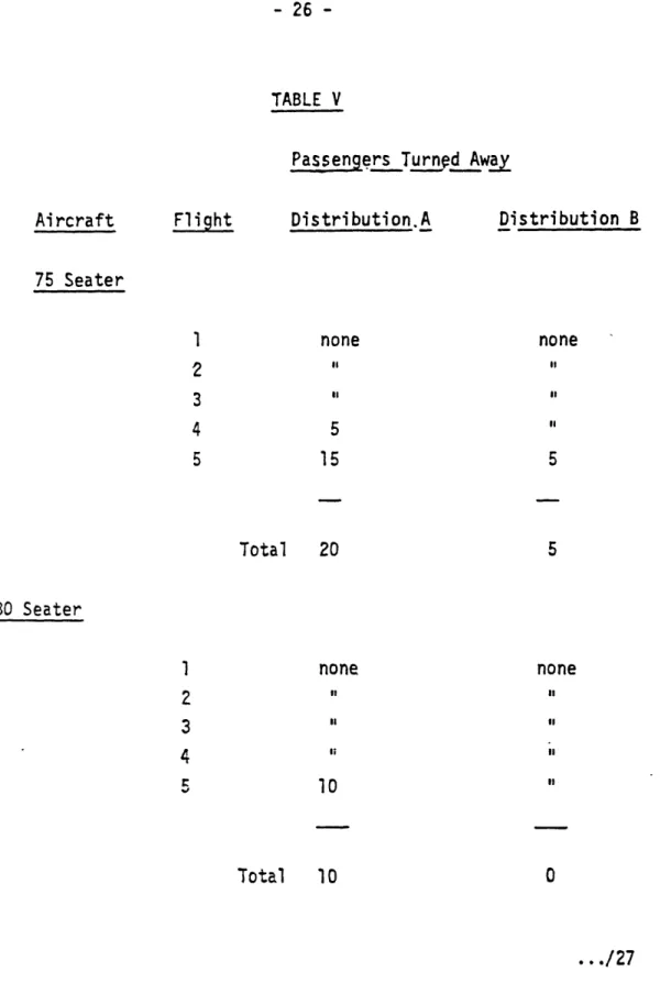
- 25 -TABLE IV Distribution A (High Variance). Average Pax 5G 60 70 80 90 70 Distribution B (Low Variance) Average Pax 60 65 70 80 80 70
The two distributions given above have the same average values but
differ in their variance. If we compare the operation of two aircraft
on two routes represented by these two distributions, the first of size
75 seats and the second of size 80 seats, the number of passengers turned
away because of lack of capacity on the aircraft will be as follows: Flight 1 2 3 4 5 Average
m moullwilililligIii Ill I Ill I I j, I Ill i 1611111WIN14 I'll Ul
TABLE V Passengers TurnpdAwy Distribution.A none Distribution B none Total 20 80 Seater none it Total 10 Aircraft 75 Seater Flight none il
- 27
-It can thus be seen that the larger aircraft shows a greater revenue
gain when traffic distribution has a high variance. In this particular
case the larger aircraft showed a gain of ten passengers in the high variance
distribution but only five in the low variance distribution.
This particular case has been chosen as the subject of
Illustration II on page 76.
The Summary of Results given on pages 78 and 79 demonstrates
that the gain by the larger aircraft operating equal frequencies varies substantially depending on changes in market conditions. Under certain conditions, the gain becomes sufficient to cover the higher cost of operation.
Equally, it can be seen that, on the basis of equal capacity, the total gain by the smaller aircraft varies, but with a lesser magnitude, with changes in market conditions. Therefore no general
judgement can be made for or against a particular aircraft. It will
always depend on the particular airline's network, different route
traffic densities and competition.
C- In a bilateral negotiation between two countries agreement
was reached between the two sides that the expected traffic would ,
amount to 1000 passengers per week in each direction. This would
mean that each airline should mount capacity equal to 1000 seats,
or a total of 2000 seats by the two airlines, resulting in a
combined load factor of fifty percent.
A problem arose however when discussion turned to the types of
aircraft and the frequencies to be mounted by each airline. One of them had 747's with a capacity of 340 seats while the other had 707's with 140 seat capacity. The second airline took the position that it should be allowed 7 weekly flights making a total of 980 seats, and that the other airline should be allowed only three flights of a total capacity of 1020 seats.
The wide body operator objected to this proposal on the grounds that the vast difference in frequency between them give the other
-carrier a tremendous advantage. To this the other airline countered by suggesting that the wide body operator had two advantages, the
- 29
-greater passenger appeal of the wide bodied aircraft, and also, the lower cost per seat on the wide body jet.
The argument thus turned into an assessment of the relative advantages of frequency against capacity, which was the subject of Case B above, and of the significance of the passenger appeal element.
It would be generally readily conceded that the question of passenger appeal is not a matter falling properly within the sphere of bilateral
negotiations but once the principle of predetermination is accepted, it would certainly be important to determine the significance of the difference in frequency.
D- In the edition of the 21st August, 1976, of Flight Magazine, the following statement appeared:
"With the same engines and flight-deck crew as the TriStar 500, the DC-10-3DR, (i.e. equipped with a RollsRoyce engine), would carry about thirty more passengers over similar stages. The TriStar 500 appears to have the edge in aircraft-mile costs, but the airlines have traditionally
placed more importance on seat-mile cost (although economic recession has taught that 30 more seats do not mean thirty more full seats). The DC-10 leads in seat-mile costs,...."
Obviously the observation that comes immediately to mind is that it would be very useful, on a matter of such importance as investment in equipment purchases of this magnitude, to provide airlines with a more scientific and serious method to assess the relative importance of aircraft-mile costs against seat-mile costs, than to rely simply on
"tradition".
Equally, if economic recession has "taught" that 30 more seats do not mean 30 more full seats, it would be extremely useful to know how many full seats do these 30 seats actually and precisely mean.
E- An airline is considering a complete reequipment program and finds that the Boeing 727-200 aircraft is the most suitable for the majority of its routes. On the remaining routes it suffers from inadequate range capability. On such ranges, its passenger capacity
- 31
-drops from the normal level of 150 seats to about 130. The airline has therefore two choices; either to decide for a mixed fleet of 727-200
and, say, 707-320 which has sufficient range for the remaining sectors, but in which case the airline will suffer a sizeable increase in costs
because of the mixture in types and the higher operating costs of the 707-320 as compared to the 727-200, or, alternatively, decide on a uniform fleet and accept the penalty of reduced payloads on the longer sectors.
It is therefore necessary to determine two unknowns:
- The magnitude of the additional expenditure arising from a
mixed fleet operation and the higher costs of the 707-320 type, as against the 727-200.
- The loss of revenue resulting from the loss of 20 seats.
As we have pointed out before, the first unknown is relatively easy to determine, especially the estimation of the higher operating costs of the 707-320 type aircraft. The estimation of the extra costs
relating to the mixing of types, is more complex and less exact. These are, in fact, several components most of which can be assessed with sufficient accuracy. The others, however, are difficult to quantify, but the magnitude of these items is relatively small and, therefore, any estimation errors can be ignored.*
The second unknown, however, that of assessing the loss of
revenue, is subject to the same uncertainties and questions that have
been outlined before.
F- An aircraft designer finds that a certain modification would
make an aircraft carry 20 percent more seats but that the cost of
operation would, as a consequence, increase by 4 percent. Is such
a modification economically attractive?
... /33
* An ingenious formula has been suggested by some aviation researchers for the assessment of the extra costs arising from mixed fleet operations:
C' = 50/N percent
where C' is the percentage increase in costs and N is the number of aircraft in the fleet. Obviously, there is no scientific method of assessing the validity of this formula.
- 33
-The answer to this question rests of course on the number
of passengers that will be carried as a result of this modification,
i.e., because of the 20 percent extra seats. If the revenue from
these passengers is greater than the 4 percent increase in cost, then,
obviously, the modification is worthwhile.
Again it should be stressed that the answer needed in such cases should relate to the whole working life of the aircraft and not to one or two years only.
G- Larger aircraft have, generally, lower seat costs, mainly because
certain cost elements do not increase at all with increases in size or
increase on a much smaller scale (economies of scale).
Air fares are usually determined by the International Air Transport Association - IATA. They are also subject to approval by the respective
governments. It is also generally accepted that Air Travel is price elastic. Price elasticity normally ranges between - 1.5 and - 2.0.
It is desired to reduce fares in a manner which would bring to the public some of the benefit accruing from the improved economics of the larger aircraft, and, simultaneously, induce a growth in demand with
obvious benefits to passenger, operator and manufacturer alike.
It is therefore necessary to measure such improvement in economics. Clearly, it is not, simply, a matter of assessing the reduction in the unit cost of production. It is a composite figure of the lower unit cost as against the lower unit revenue, as the following example will demonstrate. (Without considering, at this stage, the effects on demand of a lower price.)
TABLE.VI
Aircraft A Aircraft B
Number of Seats 150 180
Cost of One Hour Flight $3000 $3300
Revenue of One Hour Flight* $3200 $3500
Cost Per Seat $20 $18.33
Revenue Per Seat $21.33 $19.44
Profitability Rate 0.0665 0.0606
* At $ 50 per passenger/one hour flight
- 35
-The figures shown in Table VI indicate that the 180 seater aircraft has a lower unit cost by about 8.3 percent but, against this advantage, it has a lower unit revenue by 8.9 percent. Any reduction in fares can only be considered in the light of these two figures, and in this particular case no reduction can be justified.
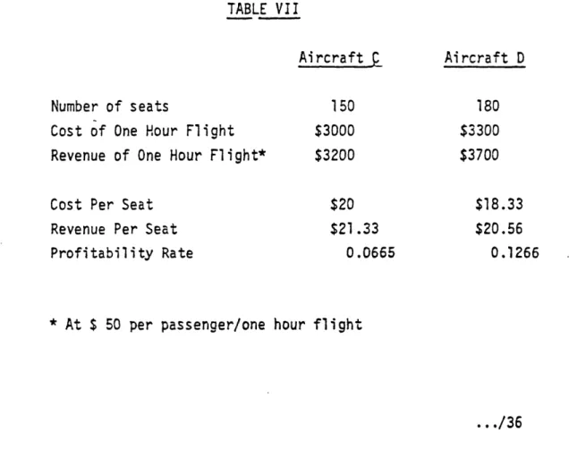
If the figures in Table VI are modified as shown in Table VII, below, there would obviously be valid grounds for a reduction in fares.
TABLE VII
Aircraft
p
Aircraft DNumber of seats 150 180
Cost of One Hour Flight $3000 $3300
Revenue of One Hour Flight* $3200 $3700
Cost Per Seat $20 $18.33
Revenue Per Seat $21.33 $20.56
Profitability Rate 0.0665 0.1266
In this case, the larger aircraft shows 8.3% lower unit cost, but
only 3.6% lower unit revenue and it is therefore possible to reduce fares
by the difference and still maintain the same rate of profitability
measured as:
Revenue - Cost
Cost
Thus, and in order to maintain the same profitability rate of 6.65%, aircraft D must earn $ 3520. It was estimated however that it
can earn $ 3700, on the basis of current fares. It can therefore be concluded that fares may be reduced by 4.86 percent.
Obviously, other factors are usually taken into consideration in
such decisions and would usually lead to a modification of this figure,
but the margin is there and is available for this purpose.
The above analysis shows very clearly that -the decision turned upon the revenue which can be earned by the larger aircraft. Aside from any difference in the passenger appeal of the two aircraft, which
- 37
-is not an issue at this point, it is a matter of assessing the extra passengers which may be carried because of the extra seats.
In Tables VI and VII the only figure that was changed was the
revenue of the larger aircraft. The figure we have been using for hourly revenue per passenger was $ 50, which means that in Table VI the larger aircraft will have to carry 6 passengers more, in order to earn the extra $ 300, and, in Table VII it will have to carry 10 extra passengers in order to earn the extra $ 500.
Thus it will be seen that our conclusions were totally dependent upon these two estimates. In other words, the basic question is whether the 30 extra seats will result in the carriage of 6 or 10 extra passengers. Again this is the question discussed in the above examples especially
B on page 18.
The Effects of Price Elasti.city
If we now add the effect of price elasticity, assumed at, say,
-1.65, the reduction of fares by 4.86 percent would translate itself
.. ./38 lviollillii III III
into an increase in demand of 4.86 times 1.65 which equals 8.019 or,
say 8%.
Evidently the smaller aircraft can only capture a smaller share
of this increase, as compared to the larger aircraft. The difference
in revenue would, therefore, be greater than the $ 320 which was arrived at in the above calculations. If it were possible to measure this
advantage with precision, the exact consequences can be quantified and the optimal decision, regarding the proposed reduction in fares, taken.
H- An airline has a mixed fleet consisting of 17 DC9s each equipped
with 110 seats and nine DC8-62s, each equipped with 180 seats. Of the nine DC8-62s, five must necessarily be deployed on certain routes where the range requirement exceeds the capability of the DC9. A decision is required regarding the routes on which the remaining four DC8-62 aircraft will be utilized.
The first reaction would obviously be that the larger aircraft must be used on those routes on which the higher load factors were achieved. Further examination, however, would show that this is not necessarily
- 39
-correct and that various other considerations must be taken into account
such'as constraints on traffic rights limiting capacity and/or frequency, traffic flow variances on the route, etc...
It is possible, for example, to find, after proper analysis,
that the DC8 would be better utilized on a higher frequency route so that the extra capacity it offers can be used to reduce flights and thus save costs.
Also, it maybe found that the DC8 can best be used on routes
with frequency limitations.
Again, analysis may show that the DC8 can best be operated on routes with high traffic flow variance although such routes show a comparatively lower average load factor. Tables IV and V of example
B (see pages 25 and 26) illustrate the significance of variance in this particular context.
The Search for a Solution
An airline executive faces this type of problem almost every day.
Without a reliable scientific method of measurement, he is obliged to
resort to such subjective approaches as judgement, concensus of opinion,
etc.
Obviously, this is a most unsatisfactory state of affairs. The search was thus started for a more satisfactory solution. In 1969, the
basic concept of the ASNA formula was established. It then took about
two years to develop the full formula and test its validity, reliability
and scope of applicability.
In its final form, the ASNA Formula provides a scientific method for the measurement of the impact on revenue and earnings of a change in capacity of aircraft and/or in frequency of operation.
Specifically, the applications of the Formula extend to:
- 41
-1- Choosing the type or types of aircraft most suited to an airline's
network and different route traffic densities. (c.f. Example B
page 17 and Example D page 29)
2- Determining the optimum combination of frequency and capacity
on a given route or route segment. (c.f. Example B page 17 and
Example C page 28)'
3- Determining the most economic deployment of an available fleet
to the airline's network. (c.f. Example H page 38)
4- Determining the optimum fleet composition and mix, i.e., how many
types and in what proportions. (c.f. Example E page 30)
5- Evaluating a proposed modification resulting in an alteration in the capacity of an aircraft. (c.f. Example A page 15 and Example F page 32)
6- Assessing the effects of alternative route authorizations and
constraints. (c.f. Example C page 28)
7- Evaluating the relationship between the size of an aircraft,
its seat costs, and fares. (c.f. Example G page 33)
Statement of Inputs
The following is the input form for the application of the ASNA
formula:
- 43
-INPUT FORM -. ASNA FORMULA
(Sector 5)
0. Base Period P
0.1. Data Relating to Airline X Average Seating on Aircraft Average Weekly Frequency
Frequency Distribution of Passenger Load Factor on Flights of
Airline X during Period P
90.0 80.0 70.0 60.0 50.0 40.0 30.0 20.0 10.0 00.0 100% 89.9% 79.9% 69.9% 59.9% 49.9% 39.9% 29.9% 19.9% 9.9% 0.2. Data Relating to All Airlipes on Sector S
Average Seating on Aircraft Average Weekly Frequency
Combined Passenger Load Factor
... /44
w fiwikw IMMINNIIi1. Alternative Ope
1.1. Data Relating to Airline.X
Average Seating on Aircraft : ... .... Average Weekly Frequency :...
1.2. Data Relating to All Airlines on the Sector
-Average Seating on Aircraft : ... . Average Weekly Frequency : ... .
2. Alternative Two
2.1. Data Relatjng to Airline X
Average Seating on Aircraft : ... .
Average Weekly Frequency : ... .
2.2. Data Relating to All Airlines on the.Sector Average Seating on Aircraft : ... Average Weekly Frequency : ...
- 45
-3. Growth Rates
3.1.
3.2.
3.3.
For Airline X under Alternative One For Airline X under Alternative Two For Total Market regardless of
Alternative
Explanations and Definitions
Sector S
Sector means a pair of points, in a given direction, regardless of whether the routing is with or without intermediate stops, and regardless of whether the flight originates or terminates at either of them. A flight with the routing Rome-Paris-New York-San Francisco would have the following pairs of points:
Rome-Paris Paris-New York
New York-San Francisco Rome-New York
Paris-San Francisco Rome-San Francisco
Therefore, and assuming that the carrier concerned has the right
to carry traffic on every one of these pairs, the ASNA formula would
have to be applied separately to each pair and in each direction. All
flights by Airline X on the pair under consideration would be included.
All flights by other carriers on that pair and in that direction would
also be included when collecting data for "All airlines on the Sector".
It should be noted, however, that when considering, for example,
the Rome-Paris sector in the above illustration, a hypothetical aircraft
should be assumed whose seating capacity will be a fraction of the
actual aircraft equal to the ratio represented by the Rome-Paris
passengers to the total passengers carried on the aircraft on that
particular sector.
Example: Assume that during the flight Rome-Paris, there were 39 pax going only from Rome to Paris out of a total of 90 pax on board the aircraft.
- 47
-Then if the total seats on the aircraft is 135. we would assume
that the carrier was operating a smaller aircraft whose capacity equals
135 X 39/90 = 58.5 , and on which 39 pax only were carried. Obviously, this smaller aircraft would have the same pax load factor
as the original one.
If Airline X operates several flights on this sector, the
above procedure must be followed for them all. Obviously, this can be
done for each flight separately, or, globally by calculating total Rome-Paris pax on all the flights and then expressing this number as a fraction of the total pax on board these same flights.
The total capacity of all these flights is then calculated,
and a fraction of it, equal to the pax fraction, is derived. This number is then divided by the frequency to arrive at the average seating
capacity as we shall see below.
For data relating to all airlines, we would include all flights
serving the sector under consideration and without apportionment of the
... /48
capacity over the various origin/destination combinations as has been done for Airline X.
The following examples will illustrate the variety of flights
which will be included.
Airline Routi . . Frequency
aaa Athens-Rome-Paris-London 7
bbb Rome-Geneva-Paris 5
ccc Beirut-Rome-Paris-New York 3
ddd Karachi-Rome-Paris-London-Montreal 4
eee Cairo-Rome-Paris-Los Angeles 2
fff Rome-Paris 5
ggg Athens-Rome-Geneva-Frankfurt-Paris 3
- 49
-(0) Base Period P
The calendar year represents the complete cycle of airline operations, while the scheduling and product marketing unit is the week.
The week is also of special significance in terms of the
interchange of passengers between flights. Market observations and research indicate that such passenger interchange, originating in flight overflows, takes place on a scale inversely related to the time interval between the flight of their first choice and the other available flights of the same airline or of other airlines serving the particular market, and that beyond a time span of one week, the
interchange becomes practically negligible.
The week was therefore adopted as the standard unit of time for the application of the ASNA formula. This entails that the input data for the base year must be converted into weekly units. Obviously, averages for periods of time or for a number of flights would suppress
the effects of chance and of basic demand fluctuation. Consequently,
the weekly units representing the Base Year (or any other period) can
be, if a certain loss of accuracy is acceptable, any of the following alternatives which have been arranged in order of level of accuracy.
1. The most satisfactory result is obtained by dividing the base year into fifty-two weeks and making a separate application for each of these weeks, resulting in a total of 104 applications to cover the two directions.
2. Almost equally satisfactory would be the random selection of, say, twelve out of the fifty-two weeks of the base year and applying the formula to each of the chosen weeks.
This means 24 applications.
3. Next would be the dividing of the year into twelve months
and making a separate application for each month. Under this alternative it is important to remember that all data
- 51
-on frequency must relate to weekly frequency as an average during each month. This, again, requires 24 applications for both directions.
4. It is also possible to divide the year into a few parts (say, 2,3, or 4 etc) e.g. On-Season, Off-Season, and Shoulder, and thus require only a reduced number of applications, but here again, the frequency must be the weekly frequency as explained under item 3, above. In this case, 3 applications for each direction are required; a total of 6.
5. It is equally possible to divide the year first into its fifty two weeks and then regroup them into any number of homogenous groups, which need not all be of equal size, and then calculate averages for each of these groups and apply the formula to them. The two directions could be grouped differently.
6. Finally, the whole year could be taken as one unit and the averages calculated as required by the ASNA Input Form.
This means two applications in all.
For clarity, we point out that the difference between
alter-natives 4. and 5. lies in the fact that under 4. the weeks in each group are in sequence (consecutive) while this is not the case under
alternative 5. To further illustrate this point we give the following examples:
Under alternative 4., the year could be divided into three
parts as follows:
Part 1: Oct 14th - Mar 16th = 22 weeks Part 2: Mar 17th - Jun 8th = 12 weeks
Part 3: Jun 9th - Oct 12th = 18 weeks
While under alternative 5., the year could be divided into the following groups of weeks:
- 53
-Group 1 : Containing 23 weeks as follows:
8 weeks Oct 14th - Dec 8th
9 weeks Jan 20th - Mar 23rd 6 weeks Apr 28th - Jun 8th
Group 2 : Containing 17 weeks as follows:
1 week Dec 9th - Dec 15th 2 weeks Dec 23rd - Jan 5th 1 week Jan 13th - Jan 19th 1 week Mar 24th - Mar 30th 1 week Apr 7th - Apr 13th 1 week Apr 21st - Apr 27th 3 weeks Jun 9th - Jun 29th 3 weeks Jul 14th - Aug 3rd 3 weeks Aug 18th - Sep 7th I week Oct 6th - Oct 12th
... /54
Group 3 : Containing 12 weeks as follows:
1 week Dec 16th - Dec 22nd 1 week Jan 6th - Jan 12th 1 week Mar 31st - Apr 6th 1 week Apr 14th - Apr 20th 2 weeks Jun 30th - Jul 13th 2 weeks Aug 4th - Aug 17th 4 weeks Sep 8th - Oct 5th
The general principle underlying these divisions or groupings
is that the accuracy of the ASNA formula increases with a higher degree of homogeneity between the weeks for which average figures are being utilized. The term homogeneity in this context refers to
the absence of major differences or changes, for the whole market,
between one week and another in terms of:
1- Frequency
2- Size of Aircraft
3- Total Demand
- 55
-This would explain the order of preference established above. It should be noted, in this context, that the six alternatives are listed in descending order of accuracy, which is, simultaneously, in ascending order of required time, effort and cost.
Under the first alternative, every set of conditions would
require the compilation
of
104 sets of figures (two sets for each
week, one outbound and one inbound on the specified sector), while under the second alternative only 24 are used (two for each month). At the other end of the scale, in alternative 6, only two sets are needed.
In order to gain a better appreciation of the inverse
relation-ship between relative accuracy and relative cost of the various
alternative methods of compiling the input data for the Base Period,
several test comparisons were made.
As one would have expected, the results demonstrated that the
more homogenous the figures which are grouped together, the closer
is the agreement between the results obtained from the "averaged week"
and those of the "average of the individual weeks".
In other words, if we compare, for example, the results obtained
from applying the ASNA formula to one average week representing a whole
year (alternative 6) with the average of twelve results obtained,
from twelve weeks each representing an average for one month
(alternative 3), we would find that the smaller the variance between
the various monthly averages, the lesser the divergence between the
two results.
Specifically, it was noted that the grouping of flights over
any time interval would not affect the results in any appreciable
manner as long as the load factor, for all carriers on the market, remains relatively stable within that interval.
At this point, it is useful to refer to a refinement in respect of the Base Period.
- 57
-Normally, the Base Period should cover the last twelve months for which statistics are available, regardless of the alternative chosen in terms of length of period or grouping and selection.
There are cases however when the last twelve months for which statistics are available are not completely normal, having been affected by major social, economic or political events.
In such cases it would be advisable to start from the twelve months preceding such events, but, obviously, the growth rates under item 3 of the Input Form (page 35), must be adjusted so as to reflect
the additional growth during the "abnormal" twelve months that were excluded.
(0.1) Data Relating to Airline X
(0.1.1) Average Seating on Aircraft
0.1.1.1 Add all the seats on all the flights flown
by Airline X on Sector S during the Base Period P.
0.1.1.2 Divide 0.1.1.1 by 0.1.2.1 (below) to arrive at average seating per flight.
0.1.1.3 Determine total passengers travelling on all
those flights whose origin and destination is identical with Sector S.
0.1.1.4 Determine all passengers travelling on all those flights regardless of origin and
destination.
0.1.1.5 Divide 0.1.1.3 by 0.1.1.4 and multiply by
0.1.1.2 to arrive at "Apportioned Capacity of Aircraft".
- 59
-(0.1.2) Average Weekly Freguency
0.1.2.1 Determine number of all flights operated by Airline X on Sector S during Period P.
0.1.2.2 Determine number of weeks in Base Period P.
0.1.2.3 Divide 0.1.2.1 by 0.1.2.2 to arrive at
average weekly frequency.
(0.1.3) Frequency Distribution of Load Factor
0.1.3.1 Take the passenger load factors of all flights
included in 0.1.1.1 above.
0.1.3.2 Classify them by intervals of 10 percentage points as shown in the input sheet. The
calculation of "Apportioned Capacity of
Aircraft" as in 0.1.1.5 above does not affect these figures as the load factor remains the
same.
0.1.3.3 Convert into a relative frequency distribution.
(The total always being one)
(0.2) Data Relating to All Airlines on. SectorS
(0.2.1) Average Seating on Aircraft
0.2.1.1 Add all the seats on all the flights flown by
all airlines, other than Airline X, on Sector
5 during Base Period P.
0.2.1.2 Multiply 0.1.1.5 by 0.1.2.1 to arrive at
total "Apportioned" seats offered by Airline
X.
0.2.1.3 Add 0.2.1.1 and 0.2.1.2 to arrive at total
- 61
-0.2.1.4 Divide 0.9.1.3 by 0.2.2.2 (below) to arrive at average seating per flight for all
airlines, including X.
(0.2.2) Average Weekly Frequency
0.2.2.1 Determine number of all flights operated
by all airlines, other than X on Sector S
during Base Period P.
0.2.2.2 Add 0.1.2.1 to arrive at total-flights in
the Sector.
0.2.2.3 Divide by 0.1.2.2 to arrive at Average
Weekly Frequency.
(0.2.3) Combined Passenqer Load Factor
0.2.3.1 Determine Average Passenger Load Factor on
0.2.3.2 Multiply 0.2.1.1 by 0.2.3.1 to arrive at passengers carried by other airlines.
0.2.3.3 Add 0.2.3.2 and 0.1.1.3 to arrive at total passengers carried by all airlines.
0.2.3.4 Divide 0.2.3.3 by 0.2.1.3 to arrive at the combined passenger load factor.
(1) Alternative One:
Both alternatives relate to the same period of time in the future. The total market is assumed to remain constant
over the two alternatives. If a different set of market conditions is to be examined, then a different application would have to be made. The only differences between the two alternatives relate to changes in the operations of Airline X and the other airlines, as well as in the relative market position of Airline X as will be shown in the following comments.
- 63
-Data Relating to Airline X
An actually planned, or hypothetical, schedule must be taken as the basis for calculations.
1.1.1 Average Seating on Aircraft
Follow same steps as under 0.1.1 above, using the planned or hypothetical schedule.
1.1.2 Average Weekly Frequency
Follow same steps as in 0.1.2
Data Relating to All Airlines on the Sector
The Base Period inputs are modified in accordance with known planned changes of the programs of other
(1,1)
airlines plus any which may be expected and which it
is desired to consider and assess the effects thereof.
1.2.1 Average Seating on Aircraft
Follow same steps as in 0.2.1
1.2.2 Average Weekly Frequency
Follow same steps as in 0.2.2.
Alternative Two:
A different operating program, actually planned or
hypothetical, is being examined under Alternative Two, but without change in the overall market conditions assumed for Alternative One.
- 65
-Data Relating to Airline X
2.1.1 Average Seating on Aircraft
As in 1.1.1
2.1.2 Average Weekly Frequency
As in 1.1.2
Data Relating to All Airlines on the Sector
2.2.1 Average Seating on Aircraft
As in 1.2.1
2.2.2 Average Weekly Frequency
As in 1.2-.2. (2.1)