HAL Id: tel-01118690
https://hal.univ-grenoble-alpes.fr/tel-01118690v2
Submitted on 18 May 2016HAL is a multi-disciplinary open access
archive for the deposit and dissemination of sci-entific research documents, whether they are pub-lished or not. The documents may come from teaching and research institutions in France or abroad, or from public or private research centers.
L’archive ouverte pluridisciplinaire HAL, est destinée au dépôt et à la diffusion de documents scientifiques de niveau recherche, publiés ou non, émanant des établissements d’enseignement et de recherche français ou étrangers, des laboratoires publics ou privés.
Very high-resolution polarimetric SAR image
characterization through blind sources separation
techniques
Nikola Besic
To cite this version:
Nikola Besic. Very high-resolution polarimetric SAR image characterization through blind sources separation techniques. Signal and Image processing. Université de Grenoble; Univerzitet Crne Gore (Podgorica, Yougoslavie), 2014. English. �NNT : 2014GRENT118�. �tel-01118690v2�
�
������
�������������������������
DOCTEUR DE L’UNIVERSITÉ DE GRENOBLE�
��������������������������������������������� ��������������������������������� � ������
��������DE L’UNIVERSITÉ ��������������
����������������������������������
�
�
���������������������������
� �
�
�
�
������������������������������������������������������� ������������������ � �������������������������������������������������� ����������������������������������������������� d’électrotechnique (ETF)�������������������� ��������������������������������
���������������������������������
������������������������������
�������������������
�
� ������������������������������������������������� ����������������������������� ������������������� ������������������������������������� ����������������������� ����������������������������������������������� ���������������������� ���������������������������������������������������� ��������������������� �������������������������������������������������� ����������������� �������������������������������������������������� M. Guy D’URSO� ���������������������������������������������� ������������������ ������������������������������������� ��������������������� ��������������������������������������������� �������������������� ������������������������������������������������������������
�T H E S I S
Very high-resolution polarimetric SAR
image characterization through Blind
Sources Separation techniques
Presented and defended by
Nikola BESIC
for jointly obtaining the
Doctorate degree
of University of Grenoble
Doctoral School for Electronics, Power Systems, Automatic Control and Signal Processing Specialization: Signal, Image, Speech, Telecommunications
and the
PhD degree in Technical Sciences
of University of Montenegro
Faculty of Electrical Engineering Specialization: Signal Processing
Thesis supervised by Gabriel VASILE,
directed by Jocelyn CHANUSSOT and Srdjan STANKOVIC.
Prepared in the Grenoble Image Parole Signal Automatique laboratory (GIPSA-lab) and partly, at the Faculty of Electrical Engineering.
Defended in Grenoble, on 21th November 2014, in front of the jury: President: Marie CHABERT - Professor, INP Toulouse
Opponents: Laurent FERRO-FAMIL - Professor, University of Rennes I Philippe RÉFRÉGIER - Professor, École Centrale de Marseille Examiners: Predrag MIRANOVIC - Professor, University of Montenegro
Antonio PLAZA - Professor, University of Extremadura Guest member: Guy D’URSO - Research Engineer, R&D EDF Supervisor: Gabriel VASILE - Research Scientist, CNRS Director: Jocelyn CHANUSSOT - Professor, Grenoble INP
Acknowledgements
Ce sera plutôt les remerciements... Ne pas dire thanks, mais merci, c’est mon devoir et mon désir.
J’aimerais d’abord remercier Messieurs Philippe Réfrégier et Laurent Ferro-Famil, les rap-porteurs de ma thèse, pour leurs analyses très appréciées des travaux effectués pendant ma thèse et présentés dans ce manuscrit. Merci à Madame Marie Chabert d’avoir accepté le rôle de la présidente du jury, ainsi qu’aux examinateurs, Messieurs Antonio Plaza et Predrag Mi-ranovic, pour leurs questions et remarques très intéressantes. C’est un grand honneur pour moi que tous ces scientifiques extraordinaires aient accepté de faire partie de cette histoire, mon histoire.
Sans aucun dilemme, le plus grand merci va à Gabriel. Si cette thèse pouvait avoir un coauteur, ce serait lui. Si on pouvait dire que, après cette thèse, on a quelqu’un qui ressemble à un scientifique, ce serait lui qui l’a créé. Si rien d’autre, il a gagné un ami fidèle.
Je suis très reconnaissant à mes directeurs de thèse, pour leur soutien sans réserve et leurs conseils qui m’ont aidé à rester sur le bon chemin. Merci à Jocelyn d’avoir eu toujours de la patience pour m’écouter, malgré le fait qu’il était toujours très occupé et moi, assez souvent, un vrai casse-pied. Merci à Srdjan pour toutes nos discussions et surtout, d’avoir été quelqu’un, dont l’opus scientifique considérable, avait ouvert la porte vers ma vie en France.
J’ai très envie de mentionner ici l’équipe des ingénieurs-chercheurs du R&D EDF. Un grand merci à M. Guy d’Urso, qui a également fait partie du jury, ainsi qu’à Messieurs Alexandre Girard et Didier Boldo, d’être toujours là pour me conseiller mais aussi pour juger le qualité de mon travail, dans un contexte un peu plus pragmatique. Un aussi grand merci va à Monsieur Jean-Pierre Dedieu, pour une collaboration qui m’a beaucoup plu et qui va, j’espère, continuer. Merci à mes parents et à mon frère, d’être toujours de mon coté. Sans eux, tout ce que j’ai fait et tout ce que je vais faire, auraient aucun sens.
Merci à toutes et à tous qui ont fait (partie de) ma vie pendant ces trois ans, de manier (le) plus ou un peu moins intime. On m’avait dit qu’il fallait ajouter au moins quelques prénoms ici, mais à moi vous semblez être trop importants pour être catalogués. Vous allez vous reconnaître de toute façon, j’en suis sûr. Et moi, je vous porterai dans mon cœur, partout et toujours... Pas comme les souvenirs d’une période merveilleuse de ma vie, mais comme la partie de l’essence, de ce qu’elle est ma vie.
Pour finir, je veux évoquer un aspect novateur de ma soutenance, qui a sans doute apporté pas mal d’émotions à la discussion. Notamment, au plein milieu de cette dernière j’ai eu un coup de mou et je suis tombé dans les pommes devant mon jury et quelques amis qui sont restés dans la salle après ma présentation. Leurs réactions formidables m’ont permis de me remettre en forme assez vite et d’ensuite continuer la discussion, mais elles m’ont surtout
ii
beaucoup touché... Jocelyn et Guy qui me réveillent, Gildas qui panique et qui court pour chercher de l’aide, Lucia qui vient pour tous nous calmer, Gabriel avec de l’eau, Fakhri avec du chocolat... Ce sont des images qui vont sûrement rester gravées pour toujours dans ma mémoire. Pas comme des mauvais souvenirs, mais plutôt comme une autre preuve (bien qu’elle n’était pas forcement nécessaire) que j’ai gagné beaucoup plus que quelques diplômes... ici, dans la capitale des Alpes.
À mes parents et leurs parents,
pour tout l’amour et tout ce que je suis.
"L’homme n’est pas une idée..."
Albert Camus, La peste
Contents
Abbreviations and acronyms ix
Mathematical notations and operators xi
Preface 1
A METHODOLOGICAL CONTEXT 5
I POLSAR image and BSS 7
I.1 SAR Polarimetry . . . 7
I.1.1 Basic principle . . . 8
I.1.2 Polarimetric decomposition . . . 11
I.2 SAR images statistics . . . 17
I.2.1 Single polarization image statistics . . . 18
I.2.2 Polarimetric image statistics . . . 20
I.3 Blind Source Separation . . . 22
I.3.1 Principal Component Analysis . . . 23
I.3.2 Independent Component Analysis . . . 24
II Statistical assessment of high-resolution POLSAR images 31 II.1 Introduction . . . 32
II.1.1 SAR interferometry . . . 33
II.2 Circularity and sphericity . . . 33
II.2.1 Circularity . . . 33
II.2.2 Sphericity . . . 36
II.3 Spherical symmetry . . . 38 iii
iv Contents
II.3.1 The Schott test for circular complex random vectors . . . 40
II.4 Results and discussions . . . 41
II.4.1 Synthetic data . . . 42
II.4.2 Very high resolution POLSAR data . . . 43
II.4.3 High-resolution multi-pass InSAR data . . . 46
II.5 Analysis . . . 48
II.6 Conclusions . . . 49
III Polarimetric decomposition by means of BSS 53 III.1 Introduction . . . 54
III.2 PCA and ICA . . . 55
III.3 Method . . . 56
III.3.1 Estimation of the independent components . . . 56
III.3.2 Roll-Invariance . . . 59
III.4 Performance analysis . . . 62
III.4.1 Data selection . . . 62
III.4.2 Synthetic data set . . . 63
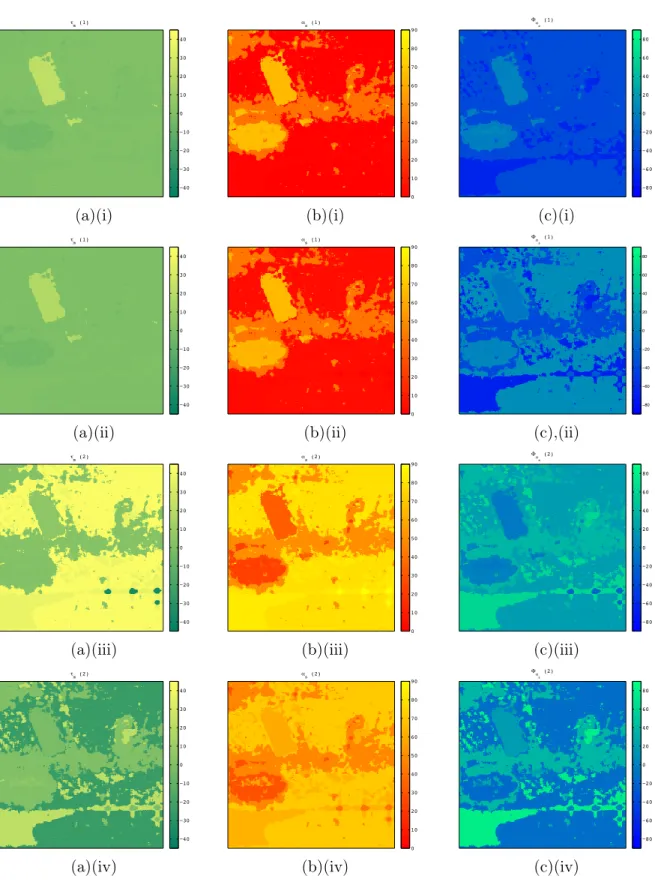
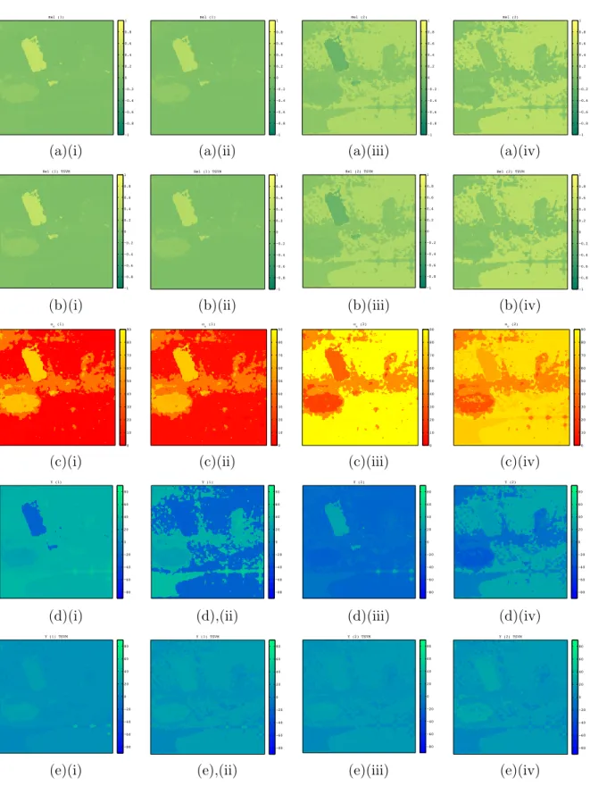
III.4.3 Data set I: Urban area . . . 64
III.4.4 Data set II: Mountainous region . . . 68
III.5 Conclusion . . . 73
Methodology: Conclusions 77 B APPLIED CONTEXT 79 IV Remote sensing of snow 81 IV.1 Snow pack properties . . . 81
Contents v
IV.1.2 Dielectric and surface roughness properties . . . 83
IV.2 Snow backscattering mechanism . . . 84
IV.2.1 Single-layer backscattering simulator . . . 85
IV.2.2 Multi-layer backscattering simulator . . . 88
IV.3 SWE hydrological modelling . . . 89
V Stochastic snow mapping using high-resolution SAR data 93 V.1 Introduction . . . 94
V.2 The preamble of the detection algorithm . . . 95
V.2.1 Input data . . . 95
V.2.2 SAR image processing . . . 96
V.3 Wet/Dry snow backscattering ratio . . . 96
V.3.1 Simulator calibration . . . 97
V.3.2 Variable threshold derivation . . . 99
V.4 Stochastic approach . . . 100
V.4.1 Confidence level . . . 102
V.5 Performance analyses . . . 102
V.6 Conclusions . . . 105
VI SWE spatial modelling using remote sensing data 107 VI.1 Introduction . . . 108
VI.2 POLSAR potential in SWE monitoring . . . 109
VI.3 Calibration of MORDOR using in situ measurements . . . 111
VI.4 Calibration of MORDOR using MODIS remote sensing data . . . 113
VI.4.1 MODIS data preprocessing . . . 114
VI.4.2 Continuous thresholding of the SWE sub-model . . . 114
vi Contents
VI.5 Results . . . 115
VI.6 Conclusion . . . 118
Application: Conclusions 121 Overall remarks and perspectives 123 A The polarimetric model of snow backscattering 125 B The Nelder-Mead simplex optimization method 127 C Résumé étendu (fr) 129 C.1 Image RSO polarimétrique et séparation aveugle des sources . . . 132
C.1.1 Polarimétrie RSO . . . 132
C.1.2 Séparation aveugle des sources . . . 134
C.2 Évaluation statistique des images RSO polarimétriques à haute résolution spatiale135 C.2.1 Paramètres statistique . . . 135
C.2.2 Résultats . . . 137
C.3 Décomposition polarimétrique par séparation aveugle des sources . . . 137
C.4 Télédétection de la neige . . . 140
C.5 Cartographie de la neige humide par les données RSO à haute résolution spatiale141 C.6 Modélisation spatiale de l’EEN par les données de télédétection . . . 144
C.6.1 Le rôle potentiel de RSO polarimétrique . . . 146
C.7 Conclusions . . . 147
D Rezime (me) 149
Publications 151
Contents vii
Abbreviations and acronyms
AML Approximate Maximum Likelihood BSS Blind Source Separation
DEM Digital Elevation Model
DERD Double bounce Eigenvalue Relative Difference DMRT Dense Media Radiative Transfer
ECD Elliptically Contoured Distributions EDF Eléctricité de France
EM ElectroMagnetic
GLRT Generalized Likelihood Ratio Test
IC Independent Components
ICA Independent Component Analysis ICTD Incoherent Target Decomposition IEM-B Integral Equation Model-B InSAR Interferometric SAR LRT Likelihood Ratio Test
MI Mutual Information
ML Maximum-Likelihood
MLC Multi-Look Complex
MLE Maximum Likelihood Estimation
MODIS Moderate-Resolution Imaging Spectroradiometer
MORDOR MOdèle à Réservoirs de Détermination Objective du Ruissellement NC FastICA Non-Circular FastICA
PC Principal Components
PCA Principal Component Analysis PDF Probability Density Function
x Abbreviations and acronyms
POLSAR Polarimetric SAR
SAR Synthetic Aperture Radar SCM Sample Covariance Matrix
SECM Sample Extended Covariance Matrix
SERD Single bounce Eigenvalue Relative Difference SIRV Spherically Invariant Random Vector
SIRP Spherically Invariant Random Process
SLC Single-Look Complex
SPM Sample Pseudo-covariance Matrix SSD Spherical Symmetric Distributions SWE Snow Water Equivalent
SWEEP Snow Water Equivalent Estimation at the Pixel scale
TD Target Decomposition
TSVM Target Scattering Vector Model QCA Quasi Crystalline Approximation
Mathematical notations and operators
Scalars are designated using italic formating, e.g. f - frequency,
with the exception of multi-letter ones, e.g. SWE - Snow Water Equivalent.
Vectors are designated using bold formating and lower case, e.g. k - target vector.
Matrices are designated using bold formating and upper case, e.g. S - scattering matrix.
Particular probability density functions are designated using calligraphic style, e.g. N or p - PDF of the normal distribution,
with p being a general notation. The operators: [·]T - transposed, [·]H - conjugated-transposed, [·]⇤ - conjugated, [·]−1 - inversed, h.i or b[·] - estimated, ˜ [·] - whitened, ¯ [·] - mean value,
| · | - absolute value - `1 norm, || · ||2 - Euclidean norm - `2 norm, E[·] - mathematical expectation, <{·} - real part of a complex value, ={·} - imaginary part of a complex value, [·] ⌦ [·] - Kronecker product,
¬[·] - negation,
[·] ⊕ [·] - exclusive disjunction.
Preface
Remote Sensing is the science of acquiring information about the Earth’s surface without an actual contact with it, by sensing and recording scattered, reflected or emitted electromagnetic energy and processing, interpreting and applying that information. It can be defined as an applied scientific discipline, comprising and relying on more fundamental domains, as signal and image processing, electromagnetics and virtually all Earth’s sciences. Nowadays, it is impossible to envisage the latter ones deprived for a wide spatial coverage of, either objects present on our planet, or processes and phenomena occurring all over its surface. This makes remote sensing an indispensable tool in the Earth observation.
The importance of this science and the necessity for its further development are emphasized by some of the biggest challenges humanity is facing in the modern age: the observed climate changes, the rapid growth of the world population, the sustainable development etc.
The significant impact of the global warming on the environment, reflected primarily through the melting of ice on the poles and in the mountainous regions, imposes the surveil-lance of the cryosphere as one of our top priorities. Aside from this, glaciers and snow cover represent significant supply of both drinking and industrial water, whose quantity can be ac-curately estimated only by means of wide spatial assessment. The vegetation, particularly the forests, being the lungs of out planet, can be preserved only through careful and regular spatial evaluation of their state. The recognized need for food production upsurge, which ought to be done by optimizing the existing agricultural regions, requires their constant and accurate monitoring. Overseeing the oceans’ surface, covering nearly 70% of the Earth, cannot be performed but by means of remote sensing.
These are just few of many examples, an effort to demonstrate the essentiality of remotely acquired information in the Earth observation. Generalizing, by saying that everything which could not be measured locally, by means of spatial sampling, depends upon remote sensing, should not be an exaggeration.
Depending on frequency of the electromagnetic (EM) waves carrying the information, we can distinguish between different types of active and passive sensors, which can be either spaceborne or airborne. Consequently, several remote sensing disciplines exist, among which, with respect to the current infrastructure, the passive optical remote sensing and the active Synthetic Aperture Radar (SAR) remote sensing could be considered as the pre-eminent ones. Optical remote sensing operates in visible and infra-red parts of the electromagnetic spec-trum. Depending on the spectral resolution i.e. how many different frequencies we use si-multaneously, we can discriminate between monospectral (panchromatic), multispectral and hyperspectral optical images. Despite the fact that it can be acquired only during the day and the constraints concerning the presence of clouds, an optical image, being the "boosted" photography, represents a vital piece of information.
2 Preface
The SAR remote sensing, operating in the microwave part of the electromagnetic spectrum, remains to be particularly attractive due to its all-day and all-weather sensing capabilities. Aside from these, the advantage of SAR is the deeper penetration of microwaves with respect to the visible light, allowing us to deduce not just surface but volume properties as well. On the other side, there are also some disadvantages, among which the principal concerns the data interpretation. Namely, unlike it is the case with the optical images, due to the different geometry and peculiar interaction with a target, we can not entirely rely on our intuition, arising from our vision sense.
Analogously to the optical remote sensing where we simultaneously use several frequencies in order to get more information about the target, in the SAR remote sensing we rather use several polarizations of the EM waves at the transmission and at the reception. This sub-discipline is called Polarimetric SAR (POLSAR) and it results in a multichannel SAR image, with each channel corresponding to a different combination of the polarizations.
In this thesis we propose mostly the contributions to the analysis and the interpretation of the SAR images, but however, we do not neglect, but rather use and demonstrate the utility of multispectral optical images, as well.
The contributions presented in this thesis are divided in two principal parts. The first part deals with the theoretical advancements and as such, is related to the interpretation of polarimetric SAR data. More concrete, it concerns the implication of the Blind Source Sepa-ration (BSS) techniques, having an aim to enhance the interpretation quality by considering the particular characteristics of the recently acquired data. As the prelude, the methodolog-ical framework for the statistmethodolog-ical assessment of these particularities is provided. The second part, dealing rather with the application - remote sensing of snow, concerns the role of SAR remote sensing in the snow mapping and finally, the Snow Water Equivalent (SWE) spa-tial modelling, performed by means of integrating the optical remote sensing datasets in the hydrological model, but still, considered in the context of POLSAR.
The particularities of the new data mostly regard the significant improvement of the spa-tial resolution i.e. the size of the smallest object which can be distinguished on the ground. This progress has an important influence on the SAR image statistics. Namely, the conven-tional assumption for the statistical model of the multichannel POLSAR image is multidi-mensional Gaussian distribution. However, the increase of the spatial resolution compromises this assumption, leading rather to the heterogeneous clutter, characterized by non-Gaussian statistics.
The dilemmas raising in the community a propos this issue could be summarized in two questions:
• Are the newly proposed statistical models truly appropriate for modelling POLSAR and other multi-dimensional SAR data sets?
• What are we exactly gaining by acknowledging the departure from the Gaussianity assumption, in terms of interpretation?
Preface 3
These two questions were a driving force for the research constituting the methodological context of this thesis.
After introducing the basics of SAR image statistics in the first chapter, in Chapter II we propose an elaborated statistical analysis, with the aim of quantitatively determining the necessity and the benefits of the altered statistical hypotheses. That is to say, we provide our answer to the first question.
The interpretation of POLSAR images principally assumes applying polarimetric decom-position, with the goal of expressing a total target backscattering as, either coherent or inco-herent, sum of more elementary backscattering components. Among different decompositions, introduced along with the SAR polarimetry concept in the first chapter, the algebraic ones, happen to be the most widely utilized in the community nowadays. Being based on the eigenvalue analysis, they are intrinsically linked to the assumption of Gaussianity of the po-larimetric SAR clutter. As it is discussed in the introduction of the methodology part, the shift from this assumption, leads to the derived eigenvector components not to be statisti-cally independent, but rather only decorrelated. Therefore, by preferably employing the most prominent BSS technique - Independent Component Analysis (ICA), introduced in the first chapter, we propose a new approach in decomposing a polarimetric data in Chapter III. This decomposition would be our answer to the second question [1].
After introducing the basics of the snow remote sensing in Chapter IV, in the following chapter we come up with a new, stochastically based snow mapping method. Although ap-plying the developed ICTD on the POLSAR images of snow regions resulted in interesting empirical conclusions, we have implicated a bit more electromagnetic properties of a snow in the context of single polarization SAR images. Namely, the snow dielectric properties depend significantly on the quantity of liquid water present in the snowpack. Consequently, the re-mote sensing techniques employed in extracting the snow pack parameters, which would be the ultimate goal of snow remote sensing, vary upon the type of snow: whether the snow is dry or wet. Therefore, in the very beginning, it is necessary to identify the type of the snow cover. In the proposed approach [2], aside from introducing a stochastic decision, we also derive a new variable backscattering threshold, discriminating the two types of snow, which is based on the backscattering simulator and the deduced backscattering mechanism, both introduced in Chapter IV.
Finally, we concentrate on the spatial derivation of SWE. Given the ill-posedness of the backscattering model inversion problem, which causes a single polarization SAR image not to be exactly useful in this context, we turn toward a conjunction of the hydrological model and the remote sensing data. As well, we briefly present the ongoing investigations of the potentials of SWE spatial modelling using POLSAR data, reinforced by implicating BSS (PCA) in the analysis of the derived parameters. However, the calibration method of the Snow Water Equivalent (SWE) hydrological model, based on the optical remote sensing data, remains the highlight of the last chapter [3]. The referent hydrological model, which required spatial calibration is introduced in Section IV.2. Chapter VI describes the proposed algorithm, and even more, serves as the demonstration of the eventual supremacy of remote sensing with respect to the local in situ measurements.
Part A
METHODOLOGICAL CONTEXT
Chapter I
POLSAR image and BSS
I.1 SAR Polarimetry . . . 7
I.1.1 Basic principle . . . 8
I.1.2 Polarimetric decomposition . . . 11
I.2 SAR images statistics . . . 17
I.2.1 Single polarization image statistics . . . 18
I.2.2 Polarimetric image statistics . . . 20
I.3 Blind Source Separation . . . 22
I.3.1 Principal Component Analysis . . . 23
I.3.2 Independent Component Analysis . . . 24
This chapter serves as an introduction to the state of the art methods which inspired us to carry out the research presented in the methodology part of the thesis. We contemplated this chapter to be their brief but systematic review. The fusion of one portion of these methods actually forms the basis of the presented theoretical contributions.
First of all, we introduce the concept of SAR polarimetry, with the particular emphasis on the most representative target decompositions. Further on, we discuss the basics of SAR and POLSAR image statistics. Finally, we introduce the family of Blind Source Separation tech-niques, by especially stressing the Principal Component Analysis (PCA) and the Independent Component Analysis.
I.1 SAR Polarimetry
The concept of radar polarimetry dates back to the early 1950s when George Sinclair, inspired by the work of Stokes and Poincaré in the XIX century, lay its cornerstone by intro-ducing the famous scattering matrix [4]. Namely, George Stokes [4] and Henry Poincaré [5] independently defined an unified formalism for representing electromagnetic waves regardless their polarization state. Relying on this formalism, the Sinclair’s scattering matrix provides information about the target "capacity" to change the polarization state of the incident po-larization waves [6].
8 Chapter I. POLSAR image and BSS
The forthcoming work by Kennaugh [7], Graves [8], Huynen [9] and the others, leaded to the establishment of radar polarimetry as a new remote sensing discipline. This was followed by an intensive technical progress, which meant the integration of the radar polarimetry into the activities of the aerospace agencies all around the world. In the beginning, mostly airborne polarimetric sensors were developed, as RAMSES (ONERA), ESAR (DLR), AIRSAR (JPL), PISAR (JAXA), CONVAIR (CCRS) etc. Soon, the space shuttle based instrument SIR-C/X-SAR (JPL) appeared as well [6]. Naturally, this huge amount of the acquired data induced significant further advancements in theory.
Further on, numerous contributions concerning the calibration techniques and particularly concerning the data analysis and interpretation have been introduced by the entire pléiaide of scientists, including Freeman, Yamaguchi, Cameron, Cloude, Pottier, Touzi etc. making POLSAR one of the most attractive research domains in the remote sensing community. New spaceborne instruments have been launched into the orbit, among which most recently: ALOS (JAXA), TerraSAR-X (DLR) and RADARSAT-2 (CCRS). The last two are still providing us valuable polarimetric data. The datasets acquired by all of these three "new" instruments, along with the RAMSES acquisitions, are being used in this thesis.
I.1.1 Basic principle
As already implied, the very purpose or radar polarimetry is to broaden the information about the target by considering its influence on the polarization of the incident EM waves.
The polarization of the EM wave refers to the spatio-temporal behaviour of the electrical field (e) i.e. to the projection of the vector’s trajectory onto the plane perpendicular to the propagation direction kEM, defined by unit vectors x and y (Fig. I.1):
I.1. SAR Polarimetry 9
(a) (b)
Figure I.2: EM polarization: (a) horizontal, (b) vertical.
e(x, y, z, t) = <nE0ej(2⇡f t− 2⇡ λz) o = exx+ eyy= (I.1) = E0xcos ✓ 2⇡f t −2⇡ λ z + δx ◆ x+ E0ycos ✓ 2⇡f t −2⇡ λz + δy ◆ y
with f being the frequency and λ the wavelength of the wave. It is actually the difference in phase between exand ey (δ = δx−δy), which determines the polarization state. For δ = {0, ⇡} we have linear polarization, δ = ⇡/2 means circular one, while all the other values indicate the general case - eliptical polarization.
Therefore, in the most representative case (full POLSAR), we transmit linearly polarized waves: horizontal (H) and vertical (V) ones (Fig. I.2a and Fig. I.2b). At the reception, we collect the scattered signals using both horizontal and vertical antennas (Fig. C.1). The most rudimentary representation of the information acquired this way is the formerly mentioned scattering matrix:
S=Shh Shv Svh Svv �
(I.2)
with each of the elements being complex i.e. representing the impact of the target on the amplitude and the phase of the EM waves. It relates the incident and the scattered EM waves, represented by the Jones vector:
j= [Ex Ey]T = h
E0xeδx E0yeδy iT
. (I.3)
10 Chapter I. POLSAR image and BSS
(a) (b)
Figure I.3: Polarimetry principal: (a) schema of the instrument, (b) the pulses at the trans-mission (T) and at the reception (R).
matrix or the Jones scattering matrix. Former is defined for the back scatterer alignment (BSA), while latter refers to the forward scatterer alignment (FSA). The difference between these two concerns the axis z. Namely, in the first case the direction of z stays the same for both incident and scattered wave, while in the second case z corresponds to kEM (Fig. I.1).
In the case of monostatic configuration, when the same platform is used both for the trans-mission and the reception, we can assume reciprocity (Shv = Svh). Therefore, the scattering matrix is often replaced by the target vector, obtained by projecting the former onto the Pauli basis:
k= p1
2[Shh+ Svv Shh−Svv 2Shv]
T (I.4)
If the target does not depolarize the incident waves, we have coherent scattering, in which case either the scattering matrix or the target vector are indeed a suitable and sufficient representation. However, if we have a certain level of depolarization, we ought to rely on the estimated (h·i) spatial covariance of the target vector, expressed through the coherence matrix: T = EhkkHi= (I.5) = 1 2 *2 4 |Shh|2+ 2<(ShhSvv⇤) + |Svv|2 |Shh|2− 2j=(ShhSvv⇤ ) − |Svv|2 2ShhShv⇤ + 2SvvShv⇤ |Shh|2+ 2j=(ShhSvv⇤ ) − |Svv|2 |Shh|2− 2<(ShhSvv⇤ ) + |Svv|2 2ShhShv⇤ − 2SvvShv⇤ 2ShvShh⇤ + 2ShvSvv⇤ 2ShvShh⇤ − 2ShvSvv⇤ 4|Shv|2 3 5 + .
Given that a partly polarized EM wave can be represented through the four elements Stokes Vector:
i=⌦⇥|Ex|2+|Ey|2 |Ex|2−|Ey|2 2<{ExEy⇤} − 2={ExEy⇤} ⇤↵T
(I.6)
the incoherent scattering can be as well represented by 4 ⇥ 4 Kenaugh or Mueller matrix, depending on the backscattering coordinate system convention. Ex and Ey would be the
I.1. SAR Polarimetry 11
complex "full" representations of ex and ey from Eq. I.2.
However, the proper exploitation and interpretation of the polarimetric information re-quires the appropriate decomposition of the backscattering process, represented either by the (projection of) scattering matrix or by the coherence matrix. The aim is to portray a target as a sum of more elementary backscatterers. Therefore, the polarimetric target decomposition (TD), due to its crucial role, undoubtedly represents the very essence of the SAR polarimetry.
I.1.2 Polarimetric decomposition
Target decomposition (TD), introduced in the first place in [9], aims to interpret polarimet-ric data by assessing and analysing the components involved in the scattering process [10]. Roughly speaking, the assessing assumes the derivation of the involved backscattering com-ponents, while the analysis dominantly concerns their parametrization. The former can be defined as: X= N X i=1 kiXi, (I.7)
with X being the scattering matrix (S) in case of a coherent target, or the coherence matrix (T) in case of an incoherent one. Both the means of deriving the components (Xi) and their parametrizations, differ for different types of decompositions. Here, we present the ones we found to be the most notable with respect to their historical and practical relevance. After-wards, in the Chapter III, we will elaborate a new decomposition, the principal contribution of this thesis.
I.1.2.1 Coherent decompositions
The most elementary approach in decomposing a scattering matrix is based on a set of Pauli matrices, originally used by Wolfgang Pauli in his theory of quantum-mechanical spin. Due to their numerous interesting mathematical properties (e.g. hermitian, unitary and commutation properties), these matrices found their applications in many domains, among which, the SAR polarimetry. In case of monostatic configuration, the scattering matrix is decomposed into standard mechanisms as:
Shh Shv Svh Svv � = p↵0 2 1 0 0 1 � +p↵1 2 1 0 0 −1 � + p↵2 2 0 1 1 0 � , (I.8)
with the complex parameters:
↵0 = Shh+ Svv p 2 , ↵1 = Shh−Svv p 2 , ↵2= p 2Shv, (I.9)
12 Chapter I. POLSAR image and BSS
making this approach a "model based" one. The first term in Eq. I.8 represent the odd-bounce scattering: flat surface, sphere, trihedral. The second one is related to the even-odd-bounce scattering without polarization change - a dihedral with the axe of symmetry being parallel to the incident horizontally polarized wave. The third one represent the scatterer which favours the cross-polarized channel - a dihedral with the axe of symmetry rotated 45◦ with respect to the incident horizontally polarized wave [6].
A slightly different model based approach is proposed by Krogager in [11]. The second component in this case rather represents a dihedral with any orientation, while the third one represents a helix. The decomposition takes form of a:
Shh Shv Svh Svv � = ejφ ⇢ ejφsk s 1 0 0 1 � + kd cos 2✓ sin 2✓ sin 2✓ − cos 2✓ � + e⌥2✓kh 1 ±j ±j 1 �� , (I.10)
with the angles φ, φs, and ✓ being respectively the absolute phase, the single (odd) bounce component phase, the orientation of the dihedral. The real coefficients ks, kd, kh are the contributions of single bounce, double bounce and helix scatterer. The latter one represents the non-symmetrical scattering i.e. the case when the target axe of symmetry doesn’t lie in the plane perpendicular to the line of sight.
However, this decomposition is usually employed in the circular basis making this a suitable point for introducing the scattering matrix projected on the circular polarization basis. In the same way the projection onto the Pauli basis leads to the target vector, the projection onto the circular polarization ones, gives us the circular scattering matrix, which for the monostatic configuration takes the following form:
SC = Sll Slr Srl Srr � = 1 2 Shh+ 2jShv+ Svv j(Shh+ Svv) j(Shh+ Svv) −Shh+ 2jShv + Svv � . (I.11)
The lexicographic ordering of the these elements leads to the circular target vector:
kC = h Sll p 2Slr Srr iT . (I.12)
The most representative algebraic coherent decomposition would be the Cameron decom-position [12]. In this approach we cannot actually assume reciprocity, meaning that we have to consider all four elements of the scattering matrix. The decomposing process can be roughly divided on two steps:
• The first step is related to the target geometrical properties. More precisely, we are initially trying to isolate the symmetric scattering from the non-symmetric one. By maximizing the former and consequently, minimizing the latter one, we can express the scattering matrix as:
I.1. SAR Polarimetry 13
S= Smaxsym+ Sminnon−sym (I.13)
with: Smaxsym = ↵01 0 0 1 � + (↵1cos 2 + ↵2sin 2 )1 0 0 −1 � , (I.14) and
Sminnon−sym= (↵1sin 2 − ↵2cos 2 )0 1
1 0 �
. (I.15)
The ↵ parameters correspond to the ones introduced in Eq. I.9 and is the rotation angle with respect to the reference basis.
• The second step would be algebraic, given that it represents one sort of the parametri-sation of the symmetric part. Namely, if we express the matrix given in Eq. I.14 as:
Smaxsym =1 0 1 z �
. (I.16)
we can define a vector:
λ(z) = p 1 1 +|z|2 1 z � . (I.17)
Finally, if we define elementary reflectors in terms of z (e.g. z = {1, −1,1
2, −12} corre-spond respectively to sphere, dihedral, cylinder, narrow dihedral), the symmetric target can be categorized by calculating the closeness to these elementary reflectors:
λ(z) = p 1 1 +|z|2 1 p 1 +|zref|2 |1 + z⇤z ref|. (I.18)
I.1.2.2 Incoherent decompositions
Unlike it was the case with the coherent decompositions, here we are rather concentrated either on the already introduced coherence matrix, or on the covariance matrix, derived as the spatial covariance of the lexicographic target vector kc:
C = E⇥kckHc ⇤ = ⌧h Shh p 2Shv Svv iT h Shh p 2Shv Svv i⇤� = (I.19) = *2 4 |Shh| 2 p2S hhShv⇤ ShhSvv⇤ p 2ShvShh⇤ 2|Shv|2 p 2ShvS⇤vv SvvShh⇤ p 2SvvShv⇤ |Svv|2 3 5 +
14 Chapter I. POLSAR image and BSS
The first incoherent decomposition was proposed by Huynen in [9], and it assumes decom-posing the scattering as the incoherent sum of the fully polarized mechanisms and the fully unpolarized ones. Originally, the decomposition is based on Mueller matrix formalism:
M= Mpol+ Munpol (I.20)
but the same reasoning can be equally applied on either covariance or coherence matrix. The polarized matrix is then parametrized using nine parameters, among which only two are invariant with respect to the rotation around the line of sight.
The counterpart of formerly presented decompositions on standard mechanisms, in case of incoherent targets, are Freeman [13] and Yamaguchi [14] decompositions.
Freeman decomposition assumes decomposing the covariance matrix into the sum of first-order Bragg, double bounce and volume scattering:
C = Cs+ Cd+ Cv = (I.21) = fs 2 4 β2 0 β 0 0 0 β 0 1 3 5 + fd 2 4|↵| 2 0 ↵ 0 0 0 ↵⇤ 0 1 3 5 + fv 2 4 1 0 1/3 0 2/3 0 1/3 0 1 3 5 .
Bragg scattering would be a more elaborated odd-bounce backscattering, which can provide us with some details about the surface dynamics. The real parameters β, fs, fdand fv, and the complex parameter ↵, figuring in Eq. I.22 are supposed to be derived from a set of equations:
h|Shh|2i = fsβ2+ fd|↵|2+ fv (I.22) h|Svv|2i = fs+ fd+ fv
hShhSvv⇤ i = fsβ+ fd↵+ fv/3 h|Shv|2i = fv/3.
However, there is one more unknown variable than there are equations. Therefore, in order to make this a well-posed problem, we need to consider the sign of hShhSvv⇤ i − h|Shv|2i. If it is negative, we take ↵ = −1, if not β = 1.
In case of Yamaguchi, there is an additional fourth component, representing non-symmetric, helix backscattering:
Ch = fx 4 2 4 1 ±jp2 −1 ⌥jp2 2 ±jp2 −1 ⌥jp2 1 3 5 . (I.23)
I.1. SAR Polarimetry 15
Another difference would be a complex β parameter, making Cs31 to be rather β
⇤. In this case, we have a system of five equations:
h|Shh|2i = fs|β|2+ fd|↵|2+ 8 15fv+ fc 4 (I.24) h|Shv|2i = 2 15fv+ fc 4 h|Svv|2i = fs+ fd+ 3 15fv+ fc 4 hShhSvv⇤ i = fsβ+ fd↵+ 2 15fv− fc 4 1 2= {hShhS ⇤ hvi + hShvSvv⇤ i} = fc 4.
Two parameters can be derived from the second and the last equation (Eq. I.25), while the rest of the system can be solved using the same hypothesis as in the case of Freeman decomposition.
The incoherent equivalents of the Cameron algebraic method would be the Cloude and Pottier [15] and the Touzi [16] decompositions. The particular emphasise will be put on introducing these two, given that the highlight of this thesis concern one incoherent target decomposition.
The first step in both of these two decompositions is the eigenvector decomposition of the target coherence matrix, allowing us to represent the total backscattering as a sum of three backscattering mechanism. Namely, given the Hermitian nature of positive semi-definite coherence matrix, the derived eigenvectors are mutually orthogonal and characterized by real eigenvalues. Each of the derived eigenvectors forms a coherence matrix with unity rank and therefore happens to be a fully polarized target vector. The corresponding eigenvalue (λ) represents its contribution to the total backscattering.
T= λ1k1kH1 + λ2k2kH2 + λ3k3kH3 (I.25) The principal difference between two decompositions would be, the second step - the parametrisation of the estimated target vectors i.e. backscattering mechanisms.
The Cloude and Pottier decomposition is based on the ↵ − β − γ − δ parametrisation of a target vector [15]: ki =|ki| exp j✓ 2 4 1 0 0 0 cos 2 i −sin 2 i 0 sin 2 i cos 2 i 3 5 2 4 cos ↵pi sin ↵picos βpiexp jδi sin ↵pisin βpiexp jγi 3
5 . (I.26)
16 Chapter I. POLSAR image and BSS
(a) (b)
Figure I.4: Poincaré sphere representation of TSVM parameters: (a) symmetric scattering (⌧m = 0), (b) non-symmetric scattering (Φ↵s = 0).
derivation of the mean backscattering mechanism (↵p), conditioned by the probabilities of ↵pi to occur in the random sequence of parameters (Pi):
↵p= P1↵p1+ P2↵p2+ P3↵p3 (I.27)
Aside from this one, very important polarimetric descriptor would be the entropy, defining the appropriateness of using polarimetry [6]:
H = 3 X i=1 −Pilog3Pi, Pi= λi P3 i=1λi . (I.28)
The value zero indicates the absolute dominance of one fully polarized mechanism, while the value one points to the completely depolarizing target.
The third polarimetric descriptor we ought to mention would be the anisotropy:
A = λ2−λ3 λ2+ λ3
= P2−P3 P2+ P3
, (I.29)
describing the relation of the second and the third estimated mechanisms.
The Touzi decomposition is rather based on the Target Scattering Vector Model (TSVM) [16].
I.2. SAR images statistics 17
Being based on Kennaugh-Huynen condiagonalization [7, 10] projected onto the Pauli basis, the TSVM [16] allows the parametrization of the target vector in terms of rotation angle ( ), phase (Φs), maximum amplitude (m), target helicity (⌧m), symmetric scattering type magnitude (↵s) and symmetric scattering type phase (Φ↵s), among which the last four
are roll-invariant: k= m|k|mejΦs 2 4 1 0 0 0 cos 2 − sin 2 0 sin 2 cos 2 3 5 2 4 cos ↵scos 2⌧m sin ↵sejΦ↵s −j cos ↵ssin 2⌧m 3 5 . (I.30)
In order to avoid an ambiguity related to the Kennaugh-Huynen condiagonalization, the range of the orientation angle is reduced to the [−⇡/4, ⇡/4], by introducing the identity:
k(Φs, , ⌧m, m, ↵s, Φ↵s) = k(−Φs, ± ⇡/2, −⌧m, m, ↵s, −Φ↵s). (I.31)
Using TSVM parameters, it is eventually possible to represent the obtained target vec-tors on either symmetric or non-symmetric target Poincaré sphere [17, 18]. In the original decomposition, they necessarily form an orthogonal basis.
Being an integral part of the decomposition we propose in the Chapter III, the Touzi’s TSVM has a very special place in this thesis.
I.2 SAR images statistics
The complex information characterizing one pixel of the SAR image represents totality of the backscattering in the corresponding spatial cell. It means that we cannot associate this value to one scatterer covering the area equivalent to one pixel, but rather to the ensemble of elementary scatterers distributed all over the same. The EM waves scattered by each of these elementary scatterers are summed coherently, which causes their either positive, or negative interference. This phenomena, due to its manifestation in the SAR image, in form of a granular noise, is called speckle effect, or speckle noise.
Using simplified mathematical formalism (e = Aejφi
e) we can illustrate this effect by representing the total received scattered EM wave as the vectorial sum of the individual scatterers in the complex space (Fig. I.5):
Atotejφtot = n X
i=1
Aiejφi (I.32)
Different random scattering amplitudes (A) and phases (φ) of the implicated elementary scatterers cause the formation of the SAR image to be rather a stochastic process. Therefore,
18 Chapter I. POLSAR image and BSS Re e� e��� Im ϕ
Figure I.5: Speckle noise.
in order to properly exploit the information contained in it, we ought to get acquainted with the statistics of the SAR image.
I.2.1 Single polarization image statistics
As it is the case with the POLSAR image, the elementary single-look (SLC) SAR image can provide complex information in each pixel, as well. This complex information can be presented in the form of amplitude and phase, but however, most commonly it is the single channel image providing intensity (I) information.
Goodman in [19] defined a fully developed speckle, characterized by the following hypothe-ses:
• the responses of each scatterer are independent,
• the amplitude and the phase are mutually independent,
• the amplitudes of each scatterer has the same probability density function (PDF), • the phases are distributed uniformly.
By adopting Atotejφtot = x+jy, under these assumptions, both the real x and the imaginary part y of the pixel value, due to the central limit theorem, converge toward the centered Gaussian (normal) distribution:
N (v|µv = 0, σv) = 1 σvp2⇡
e
v
2σ2v, v 2 {x, y}, (I.33)
with σ being the standard deviation (σ2 - variance). The amplitude A
tot is distributed ac-cording to the Rayleigh distribution:
I.2. SAR images statistics 19 R(Atot|σ) = Atot σ2 e A2tot 2σ2. (I.34)
In this case, the intensity i.e. the single-channel SAR image, expressed as I = |Atotejφtot|2 = x2+ y2, follows the negative exponential distribution:
E(I|σ) = 2σ12e− I
2σ2. (I.35)
Having a multiplicative nature, speckle cannot be neutralized by increasing the intensity. Therefore, the most elementary approach in speckle reduction would be multi-looking, where on the expense of deteriorated spatial resolution, we obtain the decrease in speckle noise. Namely, we incoherently sum the intensities of a set of SLC images, by means of the operation which can be considered as a low-pass mean filtering (spatial averaging).
The amplitude of the multi-look (MLC) SAR image, obtained by summing N SLC images is distributed according to the generalized gamma distribution [20]:
Gg(Atot|σ, N) = 2NN 2Nσ2N(N − 1)!A 2N −1 tot e −N A2tot 2σ2 , (I.36)
while the intensity follows the gamma distribution:
G(I|σ, N) = N
NIN −1
(N − 1)!2Nσ2Ne
−N I
2σ2. (I.37)
The presented Rayleigh speckle model performs very well providing homogeneous nature of the considered POLSAR clutter. However, due to the amelioration of the spatial resolution, we ought to consider the clutter to be rather heterogeneous and thus, the SAR image to be textured. The texture model of the SAR image in terms of intensity (I) is given as:
I = ⌧ j, (I.38)
with ⌧ representing the texture variation, and j the normalized intensity (j = i
σ2). Commonly,
it is assumed for the texture to be a random gamma variable [21]:
G(⌧|k, 1/k) = k
k⌧k−1
Γ(k) e
−k⌧, (I.39)
with k being the shape factor. Consequently, the intensity of the textured MLC SAR images, obtained by means of N looks, is distributed according to the K-distribution, using the modified Bessel function of the second kind (Kn(.)) [21]:
20 Chapter I. POLSAR image and BSS K(I|k, σ, N) = 2(N k) (k+N )/2 (N − 1)!Γ(k)I (k+N )−1 2 Kk−N(2pkN I). (I.40)
Analogously, the amplitude, being A =pI, follows [22]:
K(A|k, σ, N) = 4(N k) (k+N )/2 (N − 1)!Γ(k)A (k+N )−1K k−N(2 p kN A). (I.41)
I.2.2 Polarimetric image statistics
In case of a POLSAR image, the statistical analysis gets a bit more sophisticated. Namely, we cannot stay concentrated exclusively on the amplitude or the intensity of separate chan-nels. We ought to consider their relations, both in terms of phase and intensity, as well [21]. Therefore, the target vector of a reciprocal target k is supposed to follow multivariate complex Gaussian distribution [23]:
N (k|T) = ⇡1 |T|e
−kHT−1k
. (I.42)
Both real and imaginary part of each of the elements of k are assumed to have circular normal distribution [21], which was demonstrated in [24].
The coherence matrix of the multi-look POLSAR image (N looks) is estimated as a sample covariance matrix (SCM): b Tm= E⇥kkH⇤ = 1 N N X i=1 kikHi , (I.43)
and it follows the complex Wishart distribution, which has a following PDF in case of non-reciprocal target:
W( bTm|T, N) =
N3N| bTm|N −3e−NTr(T
−1Tbm)
K(N, 3)|T|N , (I.44)
with Tr(.) being a trace operator and K(N, 3) = ⇡3Γ(N )Γ(N − 1)Γ(N − 2).
The previous formulas are equally valid for the covariance matrix (C), in case of considering the lexicographic target vector (kc) rather than the Pauli one (k).
The K-distribution of the intensity of textured MLC SAR image can be generalized to the POLSAR image [25]. Firstly, we rewrite Eq. I.38 in the vectorial form:
I.2. SAR images statistics 21
k=p⌧ z, (I.45)
with z being Gaussian multivariate random vector, and ⌧ the texture defined by the distribu-tion in Eq. I.39. Then, we estimate the multi-look SCM:
b Tm = E⇥kkH⇤ = 1 N N X i=1 ⌧izizHi . (I.46)
Finally, we can represent the multivariate K-distribution of the textured MLC POLSAR data, or more concretely of the multi-look coherence matrix, as:
K( bTm|k, T, N) = 2| bTm|N −3(N k)(k+3N )/2 K(N, 3)|T|NΓ(k) Kk−3N ✓ 2 q kNTr(T−1Tb m) ◆ Tr(T−1Tb m)−(k−3N )/2 , (I.47)
where Kn(.)and K(N, 3) have the same meaning as in the Eq. I.40 and Eq. I.44, respectively.
I.2.2.1 Spherically Invariant Random Vector
Spherically Invariant Random Process (SIRP) is the univariate stochastic model. Several spe-cial cases of univariate stochastic processes (K-compound, Weibull, etc.) have been extensively studied over the years (for example in coastal radar applications) before being reunited under the common umbrella of SIRP [26].
Spherically Invariant Random Vector (SIRV) is the multivariate generalization of SIRP. It is a multiplicative model:
y=pkx, (I.48)
where x stands for multivariate Gaussian random vector, while random variable k can be distributed according to several distributions: Gamma, Inverse Gamma, Fisher, and even as a Dirac pulse. The random vector y is therefore distributed according to, respectively: K-distribution [27], G-distribution, [28], KummerU distribution [29] and finally, multivariate Gaussian distribution.
The covariance matrix of the Gaussian random vector is defined as a normalized coherency (covariance) matrix [30]:
22 Chapter I. POLSAR image and BSS
Figure I.6: Overview of presented SAR/POLSAR image statistical models.
The big advantage of SIRV in terms of generality with respect to the texture statistics [31], assures its privileged place in this thesis when dealing with the POLSAR image statistical modelling.
I.3 Blind Source Separation
Blind Source Separation (BSS) can be defined as a family of methods which aim to recover source signals from their mixture, without having any a priori knowledge of the mixing process [32]. Formally, BSS techniques use a set of observation vectors (x) to retrieve the sources vector (s) and the mixing matrix (A), which gives the share of the sources in the observed process:
I.3. Blind Source Separation 23 x(t) = 2 6 6 6 4 x1(t) x2(t) ... xn(t) 3 7 7 7 5= As(t) = 2 6 6 6 4 A11 A12 · · · A1n A21 A22 · · · A2n ... ... ... ... An1 An2 · · · Ann 3 7 7 7 5 2 6 6 6 4 s1(t) s2(t) ... sn(t) 3 7 7 7 5, (I.50)
where variable t can be related to time, space etc.
However, the criterion for separation varies upon the method being used. The pivotal classification is related to a degree of separation, in terms of statistics. That is, the sources are expected to be either mutually uncorrelated, or mutually independent. The most rep-resentative method of the former criterion would be Principal Component Analysis (PCA), introduced in this section. The latter criterion is represented by Independent Component Analysis (ICA). Given the essential role they have in this thesis, ICA methods are presented in more details.
I.3.1 Principal Component Analysis
The Principal Component Analysis, being a wide spread tool in data analysis [33], found its application in signal and image processing, as well.
The method itself is entirely based on the eigenvector decomposition of the sample covari-ance matrix of the observation data (x[n⇥1] 2 X[n⇥N ]). Namely, the principal components (PC) can be represented as rows of matrix Y[n⇥N ], derived as:
Y = ETXc, (I.51)
with the matrix E having as columns the eigenvectors of the covariance matrix, estimated using N samples of the observation data (centered with respect to the mean value µ - subscript c):
C= E[xcxTc] = 1 N N X i=1 xcixTci= 1 N(X − µx)(X − µx) T. (I.52)
The same formalism can be applied in case of complex observations, by changing trans-posing (superscript T ) with conjugate-transpose (H).
The derived principal components are mutually orthogonal and can be regarded as un-correlated. In Fig. I.7 we demonstrate the derivation of PC, in the most simple case of two-dimensional data (n = 2). The notations of the axes are not random, but however imply that PC are in fact sources in the equation C.2 (s = y). Therefore, the columns of the mixing matrix are the eigenvectors of observation data’s sample covariance matrix (A = E).
24 Chapter I. POLSAR image and BSS �� �� (a) �� �� (b)
Figure I.7: PCA: (a) observation data (x), (b) uncorrelated sources (s).
Effectively, as demonstrated, the eigenvector decomposition of the observations’ covariance matrix, is the very simple, but efficient mean of sources separation.
I.3.2 Independent Component Analysis
In terms of statistics, uncorrelation does not necessarily imply independence. Namely, we say that two random variables are uncorrelated if their covariance equals zero:
c = E[(s1−µs1)(s2−µs2)
T] = E[s
1s2] − µs1 −µs2 = 0. (I.53)
This way, we can claim that:
E[s1s2] = E[s1]E[s2] = µs1µs2, (I.54)
which is not necessarily reflected on the relation of their PDFs (p):
p(s1, s2) = p(s1)p(s2), (I.55)
being simultaneously the condition of statistical independence. Actually, the condition in Eq. I.54 needs to be satisfied for higher statistical moments, not just the second one (covariance) in order Eq. I.55 to be true. The exception are the Gaussian variables, where Eq. I.54 implies Eq. I.55, given that the second moment is the highest non-zero one.
Therefore, the common point for all ICA methods would be the estimation of indepen-dent components (IC), by relaying on the probability moments higher than two, where the estimation of IC in fact means, the estimation of the mixing matrix A.
I.3. Blind Source Separation 25 �� �� (a) �� � � (b) �� � � (c)
Figure I.8: ICA: (a) simulated uniformly distributed independent sources (s00), (b) mixture (x), (c) whitened mixture (˜x).
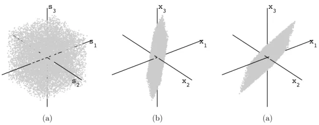
Before proceeding with the detailed elaboration, by means of slightly complicated math-ematical apparatus, we present a brief geometrical interpretation of the simplified two-dimensional scenario, given in Fig. I.8 [34]. At the same time, we present the two most important pre-processing steps: centering and whitening.
Namely, let us presume having two independent uniformly distributed sources s, with a joint scatter plot as the one in Fig. I.8a. Multiplying them with a random, non-orthogonal mixing matrix A, results in a mixture, presented in Fig. I.8b. We can consider this mixture to be the set of observation data x, making thus the aim of the algorithm, simply, to transform the data from the space given in Fig. I.8b to the one given in Fig. I.8a. The first step would be centering i.e. subtracting the mean from each of the observations’ channels, the operation which places the mixture in the centre of the "x space". Second, a bit more complex step, would be whitening i.e. the decorrelation of the observations’ channels. This is achieved by multiplying the data by the whitening matrix V:
˜
x= Vx = EDe−1/2ETx, (I.56)
where the matrix E correspond to the one used in PCA (Eq. I.51), and the matrix De is the diagonal matrix of eigenvalues. This operation gives us the joint scatter plot, illustrated in the Fig. I.8c. As it can be intuitively inferred, the only remaining operation is the rotation. This operation is, in fact, ICA. In other words, the rotation we need is contained in the demixing matrix D (inverse of the mixing matrix - ˜D= ˜A−1), and it is to be deduced from the higher order statistics. As we will demonstrate in this section, there are several means to achieve this, with most of them being based either on the iterative algorithms, or on the tensorial calculus.
The very important restriction of ICA methods, would be their unfitness in case of Gaus-sian observations. This constraint can be easily elucidated using the same intuitive geometrical approach. Namely, as it is seen in Fig. I.9, in case of a two-dimensional joint PDF space,
Gaus-26 Chapter I. POLSAR image and BSS �� �� (a) �� �� (b)
Figure I.9: ICA: (a) Gaussian observation data (x), (b) whitened Gaussian observation data (˜x).
sian observations form a circle, the fact which does not change after centering and whitening. Therefore, estimating the appropriate rotation appears to be impossible.
Finally, in order to elaborate most representative, both iterative and tensorial, ICA meth-ods, which are employed in this thesis, we ought to start from the common point - exploiting higher order statistics [35].
The statistical order k of a random variable is characterized by the kth moment µ
k and
the kthcumulant
k, both derived from the characteristic function φ(!) of a random variable:
1 X k=0 µk (j!)k k! = = φ(!) = Z 1 −1 ej!sps(s)ds (I.57) 1 X k=0 k(j!) k k! = = ln[φ(!)] = ln Z 1 −1 ej!sps(s)ds � .
Equivalent for the random vector, where we are particularly interested in the cumulant (cumk), would be:
1 X k=0 cumk (j!)k k! = ln Z 1 −1 ej!xpx(x)dx � . (I.58)
subsec-I.3. Blind Source Separation 27
tion, is focused on the statistical properties of the source as a random variable. Therefore, in this case, the higher orders are exploited by means of parameters derived in Eq. I.58. On the other side, the tensorial methods are rather based on the higher order cumulants of the observation data. Them being a set of random vectors, this approach is rather relaying on the formalism emerging from Eq. I.58.
I.3.2.1 FastICA
The FastICA algorithm is a fast converging algorithm based on a fixed-point iteration scheme. Principally, the concept of FastICA is derived from the Central Limit Theorem. It states that the distribution of the sum of two independent random variables will always be closer to Gaussian than the original variables. Therefore, the independence of the components is ensured by maximizing the non-Gaussianity of the sources [36].
There are several criteria of Gaussianity measure (fng) and therefore several approaches, used in the FastICA algorithm:
• The kurtosis criterion: Being defined in its excess (normalized) form as the ratio of 4th and 2nd order cumulants, the kurtosis of a Gaussian variable equals zero:
kurt(s) = 4 2 = µ4−3µ 2 2 µ2 2 (I.59)
Therefore by maximizing the kurtosis of each of the sources, we maximize as well their independence with respect to the other sources.
• The negentropy criterion: The Gaussian variable has the largest entropy among all the random variable with the same variance. The approximated negentropy [37], a quantity being different from zero in case of non-Gaussian variable (⌫), is defined using any non-quadratic function G(x) [34]:
J(s)/ (E[G(s)] − E[G(⌫)])2 (I.60)
Using FastICA routine [34], we are ensuring the sources independence by maximizing the negentropy.
• Mutual Information (MI) is a natural measure of the dependence between random variables: I(s1, s2, ...sn) = n X i=1 H(si) − H(s) = Z 1 −1 · · · Z 1 −1 f (s) log f (s) f (s1)f (s2) . . . f (sn) ds (I.61)
with H(s) being the differential entropy derived from the joint PDF of the sources vector as: −R1
−1· · · R1
28 Chapter I. POLSAR image and BSS
The aim in this case is to achieve zero value, which indicates independence between the sources.
• Maximum Likelihood Estimation (MLE) [38]: The log-likelihood function in the noise-free ICA model is given as [39]:
L = T X t=1 n X i=1
log fi(wTi x(t)) + T log | det W|˜ (I.62) After estimating the probability density function fiof the sources (s1...sn), the discrim-ination between independent sources is achieved through maximizing the log-likelihood function.
The columns of the mixing (de-mixing) matrix are estimated either separately or simulta-neously by iteratively searching the maximum of non-Gaussianity of the source using centered and whitened observation data:
max wi Jng(wi) =max wi E⇥fng(wT i x)⇤ ,˜ (I.63)
with wi being the column of the estimated mixing matrix, converging to the column of ˜A. In case of complex observation data, the criteria of non-Gaussianity are defined analogously but however slightly differently, as it will be discussed in the Chapter III.
I.3.2.2 Tensorial methods
The most intuitive way to introduce tensor would be representing a matrix as a 2nd order tensor. Therefore, a covariance matrix represents a second order cumulant tensor, composed of 2nd order cumulants cum
2, while a 4th order cumulant tensor (F) consists of 4th order cu-mulants cum4. Presented tensorial decomposition could be regarded as the 4thorder algebraic equivalent of the 2nd order eigenvector decomposition.
Forth-Order Blind Identification (FOBI)is one of the simplest tensorial ICA methods [40]. The independent backscattering mechanisms are derived as eigenvectors of the kurtosis matrix, estimated using a whitened set of observation vectors (˜x), as the fourth order cumulant tensor of the identity matrix I:
KI(˜x) = F(I) = E⇥(˜xTI˜x)˜x˜xT⇤ − 2I −tr(I)I = E ⇥|˜x|2x˜˜xT⇤ − (n + 2)I. (I.64) The most notable drawback of this method would be the condition that all the sources must have quite distant kurtosis values, implicating the failure in case of having several mechanisms characterized with the same distribution.
I.3. Blind Source Separation 29
Joint Approximate Diagonalization of Eigenmatrices (JADE)is a generalization of FOBI [41]. Replacing the identity matrix with a set of tuning matrices (eigenmatrices of the cumulant tensor:{M1, ...Mp}) results in a set of matrices: {KM1, ...KMp}. The whitened
de-mixing matrix ˜Dis estimated by jointly diagonalizing these matrices, which reduces to the maximization problem: max ˜ D J ( ˜ D) =max ˜ D p X i=1 ||diag⇣ ˜DKMiD˜ H⌘||2 2 (I.65)
where ||diag(.)||2 is the squared `
2 norm of the diagonal. Given that the maximization of the diagonal elements is equivalent to the minimization of the off-diagonal ones, the resulting de-mixing matrix ˜D jointly diagonalize the set of cumulants. This algorithm overcomes the mentioned drawback of FOBI, but stays limited to low-dimensional problems.
Second-Order Blind Identification (SOBI)is, sort of, infiltrated in this section, given that it does not explicitly rely on 4th order statistics. It would be actually the counterpart of JADE in the 2nd order statistics.
In this case, the observation data are divided into several series ( ˜Xi 2 ˜X) and each of them is represented by one covariance matrix (Ci).
The mixing matrix is estimated by jointly diagonalizing a set of these sample covariance matrices of whitened observations [42]:
max ˜ A S( ˜ A) =max ˜ A p X i=1 ||diag⇣ ˜ACiA˜T ⌘ ||22 (I.66)
For all presented tensorial methods, the provided formalism is entirely appropriate in case of complex observations, after changing the superscript T with H, as it was the case with PCA.
Chapter II
Statistical assessment of
high-resolution POLSAR images
II.1 Introduction . . . 32 II.1.1 SAR interferometry . . . 33 II.2 Circularity and sphericity . . . 33 II.2.1 Circularity . . . 33 II.2.2 Sphericity . . . 36 II.3 Spherical symmetry . . . 38 II.3.1 The Schott test for circular complex random vectors . . . 40 II.4 Results and discussions . . . 41 II.4.1 Synthetic data . . . 42 II.4.2 Very high resolution POLSAR data . . . 43 II.4.3 High-resolution multi-pass InSAR data . . . 46 II.5 Analysis . . . 48 II.6 Conclusions . . . 49
In this chapter we propose a methodological framework for the statistical evaluation of the particularities of high-resolution data. It assumes the analysis of three important statistical parameters: circularity, sphericity and spherical symmetry. All three of them are considered in the context of the SIRV statistical model. The conclusions drawn after applying this framework on the POLSAR datasets, are additionally reinforced by implicating high-resolution multi-pass InSAR data set, as well.
Firstly, we introduce classical circularity and sphericity tests along with their extensions to the SIRV stochastic model. Then, we present in detail the elaborated method of quantitative assessment of the conformity of the SIRV model, based on testing spherical symmetry. Finally, the results obtained using the proposed robust tests with synthetic, POLSAR and multi-pass InSAR datasets, are presented and appropriately analysed.