ARE PCBS IN PHYTOPLANKTON AND ZOOPLANKTON AT EQUILIBRIUM WITH THE WATER IN WHICH THEY LIVE?
by
Angela Cacciola
B.A., Chemistry, Barnard College, 2015
Submitted to the department of Civil and Environmental Engineering in partial fulfillment of the requirements for the degree of Master of Science at the
MASSACHUSETTS INSTITUTE OF TECHNOLOGY September 2019
© 2019 Massachusetts Institute of Technology. All rights reserved.
Signature of author
Signature redacted
Angela Cacciola Department of Civil and Environmental Engineering, MIT
Certified by
Signatureredacted
Philip M. Gschwend Ford lrofessor of Civil and Environmental Engineering Thesis supervisor, MIT
Accepted by
Signature redacted
MASSACHUSETTS INSTITUTE Colette Heald
OF TECHNOLOGY Professor of Civil and Environmental Engineering Chair, Graduate Program Committee, MIT
ARE PCBS IN PHYTOPLANKTON AND ZOOPLANKTON AT EQUILIBRIUM WITH THE WATER IN WHICH THEY LIVE?
by
Angela Cacciola
Submitted to the Department of Civil and Environmental Engineering on August 27, 2019 in Partial Fulfillment of the Requirements for the
Degree of Master of Science
ABSTRACT
Food chain bioaccumulation of polychlorinated biphenyls (PCBs) can result in harmful
concentrations within higher trophic level organisms such as fish and humans. It is important to consider how the concentrations of PCBs in phytoplankton and zooplankton affect higher trophic organisms. It was hypothesized that polychlorinated biphenyl (PCB) concentrations within primary producers such as phytoplankton simply reflect chemical equilibrium of PCB congeners
freely dissolved in the water column and in the lipid fraction of the plankton. In this study, the freely dissolved PCBs in the water of Lake Cochituate, MA, were measured using polyethylene (PE) passive sampling strips, thereby avoiding problems associated with colloid-bound PCBs. Phytoplankton and zooplankton samples were measured to determine their PCB levels and lipid fractions. The phytoplankton were at equilibrium in the fall of 2016. The phytoplankton and zooplankton appeared close to equilibrium in the spring of 2017. The large PCB congeners measured in the spring of 2017 may have been undersaturated, consistent with the idea that rapid growth leads to phytoplankton undersaturation.
Thesis supervisor: Philip M. Gschwend
Table of Contents
Abstract 3
List of abbreviations and symbols 4
Introduction 5
Materials and Methods 7
Materials
Plankton field collection and sample composition analysis Sample naming
Phytoplankton 2016 Phytoplankton 2017 Zooplankton 2017
Phytoplankton and Zooplankton extraction Lipid analysis
Protein analysis
Field deployment of PE to measure the PCB concentrations in the water PE extraction
GC-MS analysis of all field extracts
PRC mass transfer model to determine CPE at equilibrium
Equilibrium estimates of phytoplankton concentrations from the water Selection of partition (K) and diffusion (D) coefficients from the literature
Results 19
Phytoplankton and Zooplankton Sample Composition 2016 Phytoplankton
2017 Phytoplankton 2017 Zooplankton
Lipid and Protein Contents of Phytoplankton and Zooplankton Freely Dissolved PCBs Measured in Lake Cochituate Water
PRC Corrections to Equilibrium
PCBs Measured in Phytoplankton and Zooplankton
Conclusions 29
Bibliography 31
Figures and Tables
Figure 1 South Pond of Lake Cochituate Phytoplankton Sites 7 Table I Phytoplankton and Zooplankton Sample Composition Summary 11 Figure 2 Lake Cochituate phytoplankton diatoms and copepod 21 Table 2 Chlorophyll, POC:Chl-a and C:N ratios of 2017 phytoplankton samples 22
Figure 3 Equilibrium water concentrations 26
Figure 4 Concentration of PCBs in plankton as measured and estimated the water 27 Figure 5 Concentrations in the water and phytoplankton in 2016 and 2017 at S and S8 29
List of abbreviations and symbols
CF correction factor
fpe fraction of PRCs in the polyethylene after sampler deployment flipidfraction of lipid in the dry total solids
fprotein fraction of protein in the dry total solids HOCs hydrophobic organic chemicals
Kiw lipid water partition coefficient
Koc organic carbon water partition coefficient Kow octanol water partition coefficient
PCBs polychlorinated biphenyls PE polyethylene
PH phytoplankton PM particulate matter
POC particulate organic carbon PON particulate organic nitrogen
PRCs performance reference compounds RF response factor
TS total solids ZO zooplankton
Introduction
The environmental impact of hydrophobic organic chemicals (HOCs), such as PCBs (polychlorinated biphenyls), is a matter of critical importance to humans and the rest of the ecosystem. PCBs are toxic, bioaccumulative, and persistent in the environment. Although they were banned in the USA in 1979, they remain in lakes and rivers, where they are absorbed by organic material and accumulate in the food web.
Phytoplankton form the base of the aquatic food web, so in order to understand how HOCs affect higher trophic organisms, the chemical concentrations of these contaminants in the
phytoplankton must be determined. This is challenging because environmental samples are spatially and temporally heterogenous and depend on a wide variety natural and human factors. Also, many of these chemicals have low solubility in water and are therefore analytically challenging to measure.
In this work, new water passive sampling methods were applied to more accurately measure the truly dissolved concentrations of a range of PCBs in the water of Lake Cochituate in Natick, MA, in Fall 2016 and Spring 2017. Additionally, measurements of the PCB concentrations in phytoplankton and zooplankton from the same lake were made. The phytoplankton and zooplankton samples were also characterized by their fractions of lipid, protein (via nitrogen measures), and organic carbon. Plankton uptake estimates were made from the freely dissolved water concentrations using lipid-water partition coefficients, Ki. The goals were to ascertain if phytoplankton concentrations for a range of PCB congeners were at equilibrium with the water and to provide quality data to assist in the development of food web models.
Previous work
In the past, the main approach used to assess the equilibrium status of phytoplankton was to measure the chemical in whole phytoplankton, normalize the concentration to lipid content, and divide by the chemical concentrations in which the plankton live [40, 33, 39, 7, 51, 6, 34]. This approach assumed that the majority of the chemical body burden associates with the lipid portion. It also required a method to determine the freely dissolved concentrations in the water. The concentrations in the organism divided by the concentrations in the surrounding water were then compared with the octanol-water partition constant, Kow, to evaluate if contaminants in the plankton were equilibrated with the water.
A variety of other studies compared the ratio of concentrations and the phytoplankton and water to the log Kow [34, 38, 39, 39, 41], but none of these studies considered the truly dissolved water concentration. For example, the work of Skoglund and Swackhamer considered the accumulation of PCBs in phytoplankton cultures and field settings [41]. Ultimately, these studies found that the growth status of phytoplankton species affected the equilibrium partitioning. When plankton
growth rates were equal in magnitude to PCB partitioning rates, compounds with log Kow > 6 were under-equilibrated. Swackhamer et al. measured operationally defined dissolved
concentrations in the water, that is, concentrations that pass through a filter. This is not necessarily equal to the truly dissolved as this type of measurement does not account for the presence of colloid-bound contaminants [23].
Nizetto et al. (2012) normalized phytoplankton concentrations to organic carbon and estimated the dissolved phase of the water from the filtered water concentrations. This required the assumption that there are no colloids. Also relevant is that phytoplankton organic carbon does not necessarily reflect the organic carbon in the sediment. Other studies were plagued by a variety of problems, such as the isolation of sufficient mass of phytoplankton to measure concentrations of low solubility contaminants [50], and comparisons of time variant
measurements of water and plankton concentrations [13]. Lastly, many studies suggested that phytoplankton were at equilibrium on the basis that lipid normalized and water concentration normalized phytoplankton concentrations were linearly correlated with Kow. However, if octanol water sufficiently represents the primary sorptive material in phytoplankton (lipid), then at equilibrium the normalized concentrations should be equivalent, not simply linearly related, to
Kow.
Log Kow based food web models are used to predict concentrations in organisms when empirical measurements are not available [14, 16, 44]. These models are site specific and therefore require calibration. The main model used to estimate phytoplankton bioaccumulation [5] is based on the data of Swackhamer [41], which may be unreliable for the reasons discussed above (i.e., lack of equilibrium, inaccurate measures of truly dissolved concentrations, inappropriate values of partition coefficients). The Gobas model is the basis for the KABAM (Kow Based Aquatic Bioaccumulation Model), which is used by the Environmental Protection Agency (EPA) to estimate the bioaccumulation potential and associated mammalian risks of HOCs in aquatic food webs for regulation purposes [5, 20, 27].
Low density polyethylene (PE) sampling methods have been developed to measure the truly dissolved concentrations of hydrophobic organic chemicals in the aquatic environment [1, 9, 22,
45]. Samplers are inserted into the environment of interest so that they can absorb contaminants.
Mass transfer and equilibrium information is used to correct field measured PE concentrations for disequilibrium and infer freely dissolved water concentrations [4, 18, 35]. In this study, we incorporated these PE sampling methods with phytoplankton and zooplankton measurements to overcome some of the shortcomings of previous work. We also correct for water temperature and phase-specific partitioning in phytoplankton, i.e. considering both lipids and proteins.
Materials and Methods
Materials
All samples and extracts were stored and processed in glassware pre-combusted at 450°C for 12h. Plastic vial caps with Teflon inserts were lined with aluminum foil to limit PCB losses to the polymeric teflon. Phytoplankton samples were collected in amber or foil-wrapped bottles due to light-sensitive chlorophyll pigments.
Dichloromethane, hexane, methanol and chloroform solvents used in this study were purchased from VWR (JT Baker Ultra resi-analyzed). A target PCB calibration standard mixture (1I g/ml, EPA 20 PCB Congener Calibration Check Solution, RPC-EPA2-1 lot CJ-344) was purchased from Ultra Scientific. Injection standard compounds (100 pg/ml in hexane, PCBs-39, 55, 104,
150 and 188) were purchased from Ultra Scientific. 13C-labeled surrogate (40 [g/ml in nonane, I3CPCBs- 19, 52, 105, 167 and 170) and performance reference compounds (PRCs, 40 pg/ml in nonane, 13C-PCBs-28, 47, 52, 101, 111, 138 and 178) were purchased from Cambridge Isotope
Laboratory (Tewskbury, MA).
1 mil plastic low density polyethylene (PE) sheets were purchased for passive sampling (25.4 ptm, Film Guard by Berry Plastics, Evansville, Indiana). A 63 m mesh phytoplankton net with a weighted cod end belonged to the field work contractors, Normandeau Associates (Sea Gear Model 9000 Plankton Net, 42.5 cm x 114 cm, Melbourne, FL). Mesh lined windows were cut into the cod end to increase water flow. A 150 m Nitex-mesh zooplankton net and a lined cod-end was purchased from Aquatic Research (Simple model, 30 cm x 90 cm, Hope, ID). At the end of the cod end was a 1.2 kg ballast weight to help the net sink.
Plankton field collection and sample composition analysis
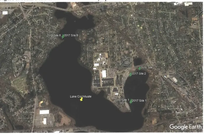
The concentrations of PCBs in phytoplankton were measured in two seasons (Fall 2016 and Spring/Summer 2017) and at two sites per season (Sites I and Site 8). Site I was chosen for its proximity to a 1980s PCB spill location, while Site 8 was chosen to determine background PCB concentrations. Zooplankton were only collected in late July of 2017. Site locations are shown in Figure 1 below.
Figure 1. South Pond of Lake Cochituate Phytoplankton Sites
Phytoplankton and zooplankton samples in this study are defined as the material collected with either a 63 pm or 150 pm net, respectively. The nets available for sampling were 21 pm, 63 Pm and 150 pm. It was expected that a 21 pm net would yield a higher detritus or dissolved organic matter to phytoplankton mass ratio. Typically, the size cut offs for collecting phytoplankton and zooplankton are operationally defined, which is why the classes of organisms collected by net towing often vary in the literature. Especially in 2017, ancillary analyses (microscope
observations, chlorophyll, TS, PM, POC, PON, silica content, lipid content, protein content) were made to further characterize sample composition.
Sample naming
In this document, samples are named according to the following indices: year collected (16 or 17), sample material (PH for phytoplankton, ZO for zooplankton, PE for polyethylene), site number (Si through S10), and sample number (.1, .2, .3, .4, .D or .E) for phytoplankton and sample type for PE with .05 for overlying water and .WC for water column). For example,
17PHS1.2 refers to the second phytoplankton sample collected from site 1 in 2017. Similarly, 17PES1.05 refers to the 0-5 cm polyethylene sample (from the water overlying the sediment) collected at site 1 in 2017.
Phytoplankton 2016
Phytoplankton were collected at Sites 1, 2, 5A and 8 by MIT-JM on November 2, 2016, near the water surface via a boat tow (Normandeau Associates, Hampton, NH). Two samples were collected per site. Each 1-L plankton sample collected was the result 3 to 4 x 1 min, 63 tm net tows at -1 mph. After each tow, there was a film covering the net and DI water was used to rinse this material into the cod end. The cod end was then emptied into the glass sample jar. The boat was then turned around and the next tow completed over the same area in the opposite direction. According to these tow specifications, samples were concentrated about 65-90 times (= volume
in cod end jar divided by the net opening area times the distance traveled). Samples were stored on ice until they were brought back to the lab in the late afternoon.
The TS (total solids) in the samples were measured to estimate the dry mass of the samples. 50 ml of hand-shaken phytoplankton samples were pipetted into ~2g tared aluminum tins and weighed. The boats were foil covered and placed in a 60°C oven until dry and then re-weighed. Density was calculated from the wet mass and volume. TS was calculated as the ratio of dry solids mass to volume of water subsampled. The DOC (OC mass from GFF filtrate/volume plankton sample) was measured by high temperature oxidation with a Shimadzu TOC-5000 carbon analyzer [32].
The lipid contents of 16PH8 were measured independently of the PCBs but via the same extraction procedure. 100 ml were extracted with DCM (detailed in the section Phytoplankton and Zooplankton Analysis below). Five, 500 tl aliquots subsampled from a 1Oml total extract volume were weighed after drying in a 60°C oven. The lipids of 16PH Iwere measured at ALS (Kelso WA), but not measured at MIT.
Phytoplankton 2017
On May 17, 2017, 40 ml of pure lake water and three 1-L phytoplankton samples were collected just below the water surface at sites I and 8. Each sample was the result of three boat tows,
each collected at 1 mph for 2 min (concentration factor -134). Qualitative observations were made of 17PH84 with a light microscope (Zeiss Axiostar Plus Microscope 4907001303). All samples were normalized for TS (Figure S1). See the 2016 methods for the protocols used. Particulate matter (PM) was measured as the phytoplankton sample solids that were retained on a glass fiber filter (Whatman, 25 mm diameter, glass fiber filter). A volumetric pipette was used to transfer 5 ml of phytoplankton sample from the middle of a shaken jar onto a single GFF (~-Ipm pore size). This was repeated three times each for samples.
The carbon and nitrogen contents of the PM at each site were measured with a CHN analyzer (Elementar Vario EL III, Mt. Laurel, NJ). 1-2 mg of dry material was removed from a sample after GFF filtration and placed into a 30 mg silver capsule (Consumers for Elemental
Microanalysis; Pennsauken, NJ) and combusted at 950°C before carbon was measured as C02
and nitrogen as N2 (hydrogen was not measured). 1-5 mg acetanilide standards (Merck KGaA,
10.1 ±0.4 %N). The background signal from 30 mg blank silver capsules was 0.0080± 0.0007%C and 0.086 ±0.005 %N (n=5).
PM samples were ashed (loss on ignition) to estimate the amount of inorganic material in each sample and reweighed for carbon and nitrogen content (Figure SI). Two PM samples from each site were baked at 450°C for 12 hours. The measured carbon and nitrogen contents of the ash were within the range of the background signal, and thus deemed negligible. Therefore, in this document, the measured carbon and nitrogen contents of the phytoplankton PM are referred to as the particulate organic carbon (POC) and particulate organic nitrogen (PON).
The chlorophyll in the phytoplankton samples was measured to estimate the POC:Chl-a ratio, a metric employed to confirm the presence of phytoplankton biomass. On the evening of field collection, the chlorophyll was extracted from the phytoplankton samples via Standard Methods [21]. 5 ml of a magnesium carbonate-saturated acetone solution were mixed with 7 ml of each phytoplankton sample. Samples were left in 4°C fridge for 80 min, then centrifuged at 1600 RPM for 20 min (Beckman Coulter Model GS-6 Swinging Bucket Centrifuge). The supernatant was poured off and the absorbances measured at 630, 647, 664 and 750 nm 5 times each in a quartz cuvette (1=1 cm) (Beckman Coulter UV/VIS Spectrophotometer, Model DU 800). In order to account for the pheophytin pigment, samples were acidified and remeasured at 665 nm. The chlorophyll in the lake water was measured as an additional estimate on the tow
concentration factor. Dilutions of the absorbance spectroscopy-determined chlorophyll concentrations (0.06 - 0.50 tg chlorophyll a/L) were used to standardize the fluorometer (Perkin-Elmer LS 50B 250). Fluorometer parameters were: 430nm excitation wavelength, 663nm emission wavelength, and beam slit width 10nm. The concentration in the lake water was measured 3 times per site against a chlorophyll-free water blank.
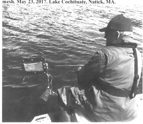
Zooplankton 2017
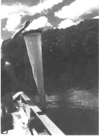
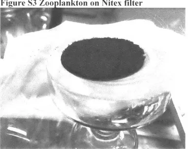
Zooplankton were collected on July 26, 2017, via repeated vertical pulls in the water from just off the bottom in 6-10 ft of water (Figure S2). The surface water temperature was 24.8°C. For each 2-liter zooplankton sample collected, the net was pulled 40-60 times by hand a vertical distance of ~3ft for a concentration factor of 20. Two, 2-L samples were collected from sites 1 and 8 (Figure S3). Each freshly collected zooplankton sample was depurated in the same lake water in which it was collected for 24 h and then filtered on a 120 tm Nitex screen to remove excreted phytoplankton (Figure S3). Samples were stored in a 10 ml vial at -80°C vial until extraction. The TS in the 120 pm Nitex screen filtered samples were weighed from 3-5 mg dry aliquots normalize zooplankton PCB concentrations on a dry mass basis (n=3). The carbon and nitrogen contents of the total solids were measured with the CHN (see 2017 phytoplankton method).
Phytoplankton and zooplankton extraction
Within three days of returning from the field, PCBs and lipids in the phytoplankton were
measured by liquid-liquid extracting a 500-700 ml of each sample (Table 1). In order to estimate the reproducibility of the DCM lipid extraction method, sample 17PHS8.4 was extracted in triplicate (200 ml x 3). All volumes were extracted three times in a separatory funnel using a
10:1 water-to-DCM ratio and I min of vigorous shaking. After agitation, the entire volume was put into the freezer overnight to break the visible emulsion. The three DCM extracts were combined into a 200 ml round bottom flask (Figure S4). A few tablespoons of anhydrous sodium sulfate were added to each extract to remove any residual water.
The PCB and lipid contents in the zooplankton were extracted in a 40 ml vial three times. The sample vials were spiked with a known amount of surrogate standard (1.5-4.5 ng of each PCB congener via a composite solution in hexane), filled with DCM, capped and incubated on an orbital shaker at room temperature. After 1 day, the DCM was drained off from the separatory funnel and stored in a glass-stoppered round bottom flask.
Phytoplankton and zooplankton DCM extracts were concentrated using a multi-port
condenser/concentration system (Starfish Multi-Experiment Work Station, Radleys Discovery Technologies, UK). The inner glass surface of the starfish apparatus was rinsed with 30 ml of DCM. The sample was attached by a ground glass fitting and concentrated for 1-2 hours at 40°C under 10-13 mmHg vacuum to ~I ml volume.
In order to measure lipid contents, the 2017 phytoplankton and zooplankton extracts were pipetted into 5 ml volumetric flasks and brought up to volume. Lipid content was determined from a 300 pL subsample, placed on a tared Al pan, gently drying, and weighing using a microbalance. The remaining DCM solvent in the extract was concentrated to ~1 ml.
A silica column cleanup was used to remove excess organic matter that would interfere with GCMS analysis. All of the extracts were solvent exchanged to hexane under a gentle steam of nitrogen at room temperature. A 30 x 1 cm glass column was prepared with a small glass wool plug, 7 g of 5% deactivated Si02 (100-200 mesh) and a ~2.5 cm anhydrous sodium sulfate cap. The sodium sulfate acts as a buffer region where the solvent can run dry without cracking the whole silica column. The column was rinsed with 20 ml DCM and then 20 ml hexane. The I ml hexane extracts were pipetted onto a silica column and three fractions eluted. Any precipitates in the concentrated extract were left in the bottom of the vial. The first fraction was eluted with 20 ml of hexane. The second fraction was eluted with 8-12 ml of 25% DCM and 75% hexane, until just before a yellow color band reached the column tip. Finally, a 20 ml 100 % DCM rinse was eluted and stored frozen. Fractions 1 and 2 were combined, nitrogen concentrated at room temperature and quantitatively transferred to an autosampler small volume glass insert with a final volume of ~25 pl.
Phytoplankton lipid analysis
Using a DCM method, the lipid and target contaminants could be extracted in one step [47]. Lipid measurements vary with solvent used for extraction and organism tissue composition. Therefore, to validate the DCM method, it was compared to the traditional Bligh and Dyer [8] and a 50% DCM:50% hexane method, previously seen to be effective in Nereis virens worms [43].
In 2016, phytoplankton samples were extracted using DCM and 50% DCM:50% hexane. 100 ml phytoplankton sample was extracted three times with 10 ml of solvent. The extracts were combined, dried with anhydrous sodium sulfate and concentrated to 10 ml. Aliquots, 100 and 500 pl (5-8) were micropipetted into tared aluminum boats and dry weights determined
gravimetrically (Cahn 25 Electrobalance, Cahn Inc. CA). The average mass extracted with the DCM:hexane solvent was 0.017 ±0.003 mg lipid/I00 d. The average mass extracted with the 100% DCM solvent was 0.018 ±0.001 mg lipid/100 p. Given the TS concentrations in each suspension, the fraction lipid in DCM:hexane solvent was 0.037. Likewise, the fraction lipid in the DCM solvent was 0.041. These were calculated by multiplying the mass of lipid in the aliquot (n=5-9) by the volume of the solvent extract and divided by the total mass extracted (POM).
In 2017, the precision of the DCM method was assessed by extracting three 200 ml subsamples from 17PH84 (see below for method). These extracts were later recombined for GCMS analysis. The average weight of nine aliquots from a 5 ml volumetric flask was 0.26 ±0.07 mg lipid/100
1l DCM (RSD=13%). The fraction lipid in the sample was 0.043.
This was compared to a Bligh and Dyer extraction on a previously frozen sample, 17PH83. The entire 630 ml sample was filtered using 12 GFFs under vacuum and then dried. 206.6 mg of dry phytoplankton were rehydrated to 80% water content (826.4 mg water) and then vortexed for 2 min with 1:2 methanol:chloroform (v/v, relative to wet sample mass). The filtrate was
transferred to a graduated cylinder and separation/clarification allowed. The top methanol layer was aspirated away and the bottom chloroform/water lipid layer (~2.1 ml) removed and filtered through a small GFF. 2ml of the remaining phytoplankton biomass was washed with ~3ml of chloroform and filtered. The filtrate was blown down with helium gas at room temperature and transferred to a 5ml vial. 100 [l extracts were removed with a glass capillary pipette, dried and weighed. This was done three times resulting in an average of 0.23 ±0.02 mg lipid/100 Pl extract.
Freezing bursts the cell membrane and likely releases many components, both colloidal and dissolved. 1.07 gdw/L was recovered by the GFF of the thawed 17PH83, which is -83% less than the 1.29 ±0.05 g/L PM measured before freezing. Therefore, the total mass extracted was increased by 17% to account for the solids lost in the freeze thaw process. If freezing broke open cells, it was assumed that the freeze-leaked matter did not include significant lipid. Thus, the
calculated Bligh and Dyer lipid fraction was 0.047. The fraction of lipid measured using the Bligh and Dyer method were within the experimental uncertainty of the DCM extraction. The fraction lipid for site 8 phytoplankton from both 2016 and 2017 as measured by different extraction methodologies (DCM, DCM:hexane, and Bligh and Dyer) was 0.042 +0.004. Therefore, we have a high degree of confidence in the DCM extraction method. Except for the
16PHS1, all other samples were measured for lipids simultaneous to the PCB extractions with only the DCM method. We use the relative deviation of the triplicate DCM extraction analysis to determine that the precision for the DCM method was 13%. Membrane lipid was not
distinguished from storage lipid, as partition coefficients of these values vary by less than one order of magnitude (Table S6).
Protein analysis
The particulate organic nitrogen (PON) was measured to estimate the fraction of protein in each sample. Chlorophyll, nucleic acids, and cytoplasmic pools of inorganic nitrogen and free amino acids can represent a substantial pool of intracellular N [30]. A ratio of 4.78 g protein/g N was used instead of the standard convention (6.25 g protein/g N) to account for all of the non-protein nitrogen associated with the sample [31].
Field deployment of PE to measure the PCB concentrations in the water
A two-piece PE sampler was constructed and deployed to measure the PCB concentrations in the water and assess their vertical distribution. Aluminum frame samplers were inserted (via a 10 ft detachable pole) with the goal that /2 to %of the PE would be in the sediment to capture the in
situ pore water concentrations near the sediment surface, and the remaining PE would sample the
overlying water concentrations. A grommeted mesh bag was floated above the metal frame with a -1 m rope and buoy to sample the water column concentrations significantly above the bed (Figure S5).
The Booij et al. protocol was followed to clean and PRC-impregnate the PE before it was loaded into the sampler frames [10]. PE strips were cut from plastic sheets to the dimensions specified in Table S1 for both samplers. The PE was cleaned by soaking sequentially in a 2-L jar with DCM and then methanol, each for 24 h. Seven PRCs were loaded into the PE via a 80:20 (v/v) methanol:water solution and incubated on an orbital shaker table at room temperature for a week to equilibrate. The strips were then soaked twice for 24 h in deionized water to remove the methanol. The aluminum frame sampler was loaded with PRC-loaded PE the night before deployment, wrapped in foil and stored on ice. Part of the excess length from each of PE
samplers were cut and reserved for t=0 PRC concentration analyses as well as some of the water column PE strips.
To assess the horizontal distribution of the PCB water concentrations each year, 10 samplers were placed along the edges of South Pond and Pegan Cove in Lake Cochituate (Table S1). In 2017, the average water depth was 6 ft, except for at site 7 where the depth was -3ft. The
samplers at sites 3 and 5 were tied to a large buoy that floated just under the surface to protect them from vandalism.
Most of the samplers were located and recovered after about two months. To minimize PCB losses to the air, recovered samplers were wrapped in aluminum foil and stored in a cooler with ice packs. Of those deployed in 2016, the sampler at site 4A was not recovered, and the sampler at site 5A was found sitting flat on the bottom. PE frames were found to have over-penetrated at Sites 2A and 9 so they only captured concentrations in the surface sediment. Of those deployed in 2017, the sampler at site 7 was lost and the sampler at site 5A over-penetrated. Lost samplers were attributed to snagging and accidental removal by fishing lines, disturbed by recreational water skiers and/or power boats or vandalism.
PE extraction
On the day following field retrievals, PE samplers were unwrapped and visually inspected. There was no visual change to the sediment side of the sampler (PE remained clear) (Figure S6).
Brown algae stained the water side, and this was wiped away with a Kimwipe@ (Kimberly Clark Worldwide Inc.). The boundary between the two was marked by a thick black line that could not be wiped away with a clean, dry Kimwipe. This likely represents the depth where subsurface sediment minerals interact with oxygenated water. Depending on the site, there may also be a layer representing constantly resuspended sediments (so called 'fluff' layer). As dissolved metals in the anoxic sediment move to the interface they likely react with oxygen and oxidize, precipitating solids on the PE. The oxide coatings could have substantially affected the mass of the PE, and thus the length scale and time of diffusion for the PCBs.
The samplers were sectioned for discrete analysis at MIT and also so that a portion of samples could be sent to ALS Environmental for external analyses (Kelso WA). The water column samplers were divided in half (each slice ~7.5 x 10 cm). The sediment sampler PEs were split into 5 or 10 cm slices according to their distance from the sediment/bottom water interface and then they were divided in half. Some samplers did not go into the sediment evenly (i.e., Site 1). In these cases, the mass of PE analyzed at ALS and MIT was usually somewhat different. The PCB concentrations in the PE slices were measured using DCM extraction. PE slices were blotted dry with a Kimwipe and each put into 40 ml amber vials. Vials were spiked with a known amount of surrogate standard (2.5-5.0 ng of each PCB congener via a composite solution), filled with DCM, capped, and incubated on an orbital shaker at room temperature. After at least 1 day, the DCM was poured off and stored in a glass-stoppered round bottom flask. The extraction was performed three times, and these extracts were combined.
All DCM extracts were concentrated using a multi-port condenser/concentration system (Starfish Multi-experiment Work Station, Radleys Discovery Technologies, Essex, UK) under 13 mmHg vacuum. ~1 ml concentrated extracts were pipetted quantitatively into 4 ml vials. The DCM
solvent in the extract was exchanged to hexane using a gentle stream of nitrogen at room temperature. The extracts were concentrated to 20-150 pL and transferred into 300 pL GCMS vial inserts. Each dried PE slice was weighed after extraction.
GCMS analysis of all field extracts
Immediately prior to the GC-MS analysis, 2.5 ng of each injection compound via a composite stock solution (25 pl of a 100 ng/ml stock solution) was added to each extract to determine final extract volumes. Standard compounds were run before, between every five, and after all field extracts. In addition to the PRC, surrogate, and injection compounds, the EPA-20 PCB mixture was analyzed to identify the target compounds and establish their response factors. Hexane blanks were run before and after standards.
PCBs were separated on a DB-5 MS 60m column (0.25 pm film thickness, 60 m x 0.25 mm ID, Agilent, Santa Clara, CA). The inlet temperature was at 300°C. Splitless, 1 l injections were made under pulsed pressure (30psi) for 1 min. The helium carrier gas had a constant flow rate of 2 ml/ min. The gas chromatograph oven was programmed to ramp from 67°C to 188 at 25°/min, from 188-276° C at 1.5 C/min and finally from 276-300° C at 25° C/min, followed by a 3.6 min hold time. The total GC run time was 68 minutes. This program reflects a balance between peak separation and total analysis time.
All of the PCBs were detected using a JEOL GCmate MS. The instrument was operated in Selected Ion Mode (SIM) mode. The mass axis was calibrated between each sample using an internal standard (perfluorokerosene, PFK). TSS 2000 software was used to integrate the peak area of the most abundant m/z ion (quantitation) of each PCB (Shrader Analytical and
Consulting Laboratories, Inc.). Baselines were corrected for automatically. The quantification and confirmation ions were used to verify each peak.
The retention times and response factors of target and standard compounds are listed in Table S2. Response factors are listed according to the groupings in which samples were analyzed. The response factor for PCBs varies based on a number of factors: the cleanliness of the injection port, the position of the column in the injection port, the condition of the capillary column, and the cleanliness of the source. These account for some of the variability in the factors seen between the 2016 and 2017 analyses.
Within a single analysis, response factors decrease with increasing congener hydrophobicity, possibly due to decreasing congener transfer onto the capillary column from the split/splitless injector. As the peak areas decrease, the compounds are more difficult to detect above
instrument background signals. Congener peaks of approximately 2000 area units/pl are
considered above background (minimum detection limit, MDL) with resulting concentrations of approximately 0.2-0.8 ng/g environmental sample (PE or plankton). Given I uL injections from
about 50 uL extracts, our reporting limits were ~0.6-1.8 ng/g, but varied with congener separation and dispersion.
On the GCMS we have measurement precision less than or equal to the RSDs of the standard curve determined RFs. The average calibration RSD for all of the analysis runs was 13 +4% (range = 8-23%). The accuracy of the RF in a given run depends on the condition of the
manufacturer stock solution and the dilution from stock to a working standard solution. The EPA 20 stock solution (RPC-EPA-2, 100 pg/mL, acetone) was obtained from Ultra Scientific (N. Kingstown, RI), an industry certified and accredited laboratory. A single dilution was made from the manufacturer stock, to obtain a 1pg/ml hexane solution which was stored in a low-loss Certan@ vial (SupelcoTM,Chromatography Division of Sigma Aldrich) to the I00ng/ml standard. All extract volumes were calculated using volume recovery corrections on a congener-chlorine number basis to negate the effects of imprecise RFis. The average volume (Vis) calculated from each injection standard was within 13% RSD (range) for all samples, which is about our
instrument calibration precision.
Injection volume (ul) = Vi, = spiking massi, RFis areai
All extracts analyzed by MIT-AC were spiked and calibrated with the same stock solution, so this method negated any imprecisions between the surrogate RFs. Larger volatilization losses during evaporation were expected for the lower molecular weight congeners. 3-Cl congeners were most sensitive to handling losses (15-50% recoveries). The average recoveries across a single congener typically reflected differences in sample handling. The uncertainty associated with making a GCMS target compound analysis was about 20%. This stemmed from the following sources: surrogate standard spiking mass (massss,(25± 2 l 8%), area surrogate standard (areass), the area injection standard (areais), the area target compound (areaT, -5% each), response factor surrogate standard (RFss, 13%,) and response factor EPA 20 compound (RFEPA, 13%).
%Surrogate Recovery = %SS= areassVis RFss spiking massss
Cr extract - areatVis _ areat massss RFsS RFEPA%SS RFEPA areas
5 areais
For the 2016 PE, the samples were not spiked and calibrated with the same surrogate stock solution. The injection and surrogate standards were assembled from high concentration
manufacturer stocks of individual congeners stored in nonane. They have been used by multiple researchers over a period of a few years and there is uncertainty regarding losses to volatility, partitioning, and contamination. This, combined with the accuracy of multiple congener dilutions to the I pg/ml stock solution, led to greater uncertainty in the extract volume and recovery calculations. The calibration surrogate standard was considered imprecise and
inaccurate relative to the EPA 20 standard. The corresponding unlabeled RFEPA 20was used in
PRC mass transfer model to determine CPE at equilibrium
A mass transfer model was used to correct for nonequilibrium of PCBs between the PE sampler and water phase (governed by 1st order kinetics) [10, 12, 42]. Specifically, the losses of PRCs from samplers to the environment were examined to determine the optimal correction for nonequilibrium conditions between target congeners in the PE and water. Targets are not initially present in the PE and PRCs are not present in the environment, therefore targets exclusively diffuse into the PE and PRCs exclusively diffuse out.
The PRC fractions remaining in the PE after their field deployments (fpe) were calculated by comparing the t=0 PRC concentrations determined from subsamples of the field-deployed PE to the PRC remaining in the PE after field deployment. In the model, it is assumed that the PRCs instantaneously disperse into the surrounding environment. When all of the PRCs have left the PE, the corresponding sized target compounds have reached equilibrium.
When the PE is less than 100 pm thick and compounds have a log Kow > 5, it is assumed that the water boundary layer controls the rate of mass transfer [9, 11, 12, 42]. The fraction of PRC in the PE can be modeled with the exponential fp= = e-kct, where Cpe is the concentration
measured in the PE [10]. In a well-mixed field site (thus infinite volume water conditions) the exchange rate coefficient, k )is equal to Kpew pe. Under water boundary layer control, the
sampling rate is R5(-) = k0A and the overall mass-transfer coefficient equals the mass transfer
coefficient for the water phase. ko = k, = ' [11, 42]. Therefore k, =Kpwg, where Dw is the diffusivity of the PCBs. D, Kpe and Lpe are measurable quantities that have been studied and reported in the literature.
The boundary layer thickness depends on the turbulence of the environment and the diffusivity of the PCB in water. The fpe,were fit with a least squares regression model to estimate a single average (this assumes solute independent boundary layer thickness even though it is ~ MW-o.24) The quality of the fit was described by the root mean squared error (RMSE). The intricacies of the fit were evaluated by comparing the measured and -calculated fractional approaches to
equilibrium, feqs.
The fractional accumulations of the target compounds were back calculated with the PRC fitted 6. The measured target concentrations in the polyethylene were then equilibrium corrected: Cpe,
eq= 1/(1-fpe)= 1/feq. The uncertainty on the Cpe,eq at each site was evaluated from two components of the PRC with the closest Kow: the RSD of the t=0 PRC concentrations and the RSD of the
PRC measured vs fitted fpe values. The Kpew was used to calculate the freely dissolved water concentrations from the CPE at equilibrium: Cw=Cpeeq/Kpew.
Equilibrium Estimates of Phytoplankton Concentrations (Cpl*) from Water Concentrations
In order to evaluate the equilibrium status of the phytoplankton and zooplankton samples with the dissolved water concentration, a sorption estimate was made based on the phytoplankton flipi
and Kiw. The reported uncertainty of the estimated phytoplankton concentrations reflected the uncertainty associated with the average water concentrations in Pegan Cove for site 1 and South Pond for site 8 and the fraction lipid (13%). When it was necessary to determine significant differences, literature reported uncertainties of the partition coefficients were considered.
Selection of partition (K) and diffusion (D) coefficients from the literature
In the absence of experimental parameters, Abraham coefficient based ppLFERS (poly parameter linear free energy relationships) and Kw based LFERS (linear free energy
relationships) were used to estimate partition constants. The van Noort updated PCB coefficients were used in place of the Abraham coefficients where possible. The lipid water partition
coefficients (Kim) were calculated with the Endo et al. ppLFER [17]. log Kim values at 25°C vary between 5.26 ±0.21 and 8.79 0.28 L water /kg lipid. The Kpw partition coefficients were calculated with the fish protein ppLFER reported by Geisler et al. [19]. The magnitude of these were 70 to 250 times smaller than their Kiipidwatercounterparts. The values of all partition coefficients are reported in tables S3 and S4.
Experimentally determined Kpew from Choi et al. were employed [15]. Otherwise the Kpewwas calculated from the Choi LFER and based on Hawker and O'Connell Kows [24] to estimate the Kpe. The uncertainty associated with the measured values averaged 0.03 log units (range 0.01-0.28 log units). The average RSD (28%) of PCBs reported in the literature was used for the Kow predicted Kpew[29]. log Kpevalues at 20°C vary between log 4.60 and log 7.89.
Several studies have considered the effects on partition coefficients of water and organic phases like PE [1, 11] and lipid [17, 19] in an effort to estimate phase specific excess enthalpies over environmentally relevant temperatures. The data are limited and do not consider the whole range of PCBs measured in this study. It was assumed that the changes in partitioning for all phases could be estimated with a AHow ppLFER [37]. The AHow for the range of PCBs studied from smallest to largest congeners ranged between -16 and -35 kJ/mol, which indicates that from 12 to 25°C, Ks decrease by a factor of 25-50%.
The diffusivity in water, Dw, was calculated from the temperature dependent (via solvent viscosity) formula of Hayduk and Laudie [25]. Comparison of these values with the
Schwarzenbach et al. relationship based on the data of Yaws [49] indicated that the Dw of PCBs can vary by 0.01-0.16 log units, depending on the source of the model: 0.11 log unit variation
Hayduk and Laudie vs Yaws relationship and 0.16 log units with 12°C change. All the values are listed in Table S5.
Results
Phytoplankton and Zooplankton Sample Composition 2016 Phytoplankton
In initial assessments of phytoplankton tow samples, there was some concern that organic matter buildup over the tow duration could decrease the net efficiency. This would adversely affect our measurement of PCB concentrations because we would be underestimating phytoplankton mass due to colloid collection. The average TS of the phytoplankton samples at Sites 1 and 8 was 670 ±90 mg/L (Table 1). The DOC accounted for ~6% of the TS, a minor fraction of the extracted mass.
2017 Phytoplankton
A sample of Lake Cochituate phytoplankton diatoms is shown in Figure 2. The composition of the Site 8 tow concentrated 2017 phytoplankton lake samples were examined via microscopy. These observations indicate that of a natural population of freshwater diatoms. The
phytoplankton samples appeared greenish brown in color. A few diatom species, Synedra,
Tabellaria, Stephanodiscus and Asterionella, dominated the microscopy fields. These same
species were observed by George Whipple in 1896 [48]. Some detritus and an isolated
zooplankton were observed among the diatoms (Figure S7). No microscope observations of Site I phytoplankton samples were made.
TS, POC, PON and chlorophyll measurements between the two sites were similar. In 17PHS8.4 phytoplankton, the measured PM accounts for 78% of the total solids in the sample. PM was relatively uniform across six samples from the two sites, with an average PM of 1.4 0.2 g/L. The PM at 17PHI and 17PH8 were not significantly different (1.4 0.2 g/L at site I and 1.5 0.2 at site 8).
The POC:PON ratios together with the ash content of the PM suggest that the sample solids comprised of diatoms (Table 1). The average C:N molar ratio of the six phytoplankton samples from two sites was 6.3 ±0.8, consistent with Redfield stoichiometry (6.6) of nutrient replete phytoplankton populations (Table 2). The differences between sites were not significant but there was some variability among samples from a single site. The average POC and PON at
17PHS Iwas 20 ±1% and 2.5% 0.3% of the PM, and the average at 17PHS8 was 23 1% and 2.9 ±0.1 (Table 1). The ash content determined at 450°C of the PM samples was not
significantly different at sites I and 8 and the average was 48 ±5%. (50 7% at site 1 and 46 6% at site 8). This was inferred to be silica based on microscope observations of freshwater diatoms.
Figure 2. (left) Lake Cochituate phytoplankton diatoms (17PHS8.4) (right) Lake Cochituate copepod (17ZOS8)
When compared with the POC, chlorophyll measurements further support the presence of phytoplankton populations (Table 2). Chlorophyll was extracted from whole water samples, and reflect the chlorophyll associated with the TS. Some variability was observed within samples from a single site. The average concentrations were similar between sites 1 and 8. In site 1, the average chl-a, chl-b and chl-c concentrations (5 replicate analyses) were 2180 50 Ig/L, 390± 90 pg/L, and 1300 80 pg/L. For site 8 the average concentrations were 2500 ±30 pg/L, 200±
100 pg/L and 1300 200 pg/L. The POC:chl-a for the six phytoplankton samples was 129 24, which is within the wide range of laboratory and field study reported values (6 - 333) [26]. These chlorophyll numbers suggest a high percentage phytoplankton mass in the sample. The chlorophyll concentration factors were 60 ±20. The chl-a extracted from the TS in sites 1 and 8 unconcentrated lake water were 50 pg/L and 30 pg/L, respectively (Table 2). These values suggest that the parameter tow concentration factor severely overestimated biomass collection. The POC:chl-a ratio from the tow samples were applied to the lake water chl-a to estimate the in
situ phytoplankton concentrations: 6 and 4.9 mg phytoplanktonPOC/L lake water (28 mg dry
phytoplankton/L lake water) at sites I and 8, respectively. These estimates are useful for determining plankton inputs in food web models.
Table 2. Chlorophyll, POC:Chl-a and C:N ratios of 2017 phytoplankton samples
Sample Chlorophyll (mg/L) POC:Chl-a C:N
chl-a chl-b chl-c
Lake Water Site 1 0.053
17PHS1.1 2.13 0.03 0.29 0.01 1.21 0.06 106 5.5 17PHS1.2 2.21 ±0.06 0.39 ±0.04 1.33 0.08 112 6.0 17PHS1.3 2.18 ±0.02 0.50 0.01 1.35 ±0.01 136 6.7 Lake Water Site 8 0.035
17PHS8.1 2.64 0.05 0.23 0.02 1.41 0.05 156 7.6 17PHS8.3 2.83 ±0.03 0.40 0.02 1.52 0.06 105 6.7 17PHS8.4 2.09 ±0.03 0.09 ±0.03 0.84 0.07 157 5.2 Average 17PHS1 2.18 ±0.05 0.39 0.09 1.30 0.08 118 16 6.1 0.6 Average 17PHS8 2.5 0.3 0.2 0.1 1.3 0.3 140 30 6.5 1.2 Average 17PH 2.4 0.3 0.3 0.1 1.3 0.2 129 24 6.3 0.8 2017 Zooplankton
A subsample from 17ZOS8.E was diluted and examined microscopically. Copepod species were observed (Figure 2). The TS of 17ZOS1.D and 17ZOS8.E were 172 and 85 mg/L, respectively. C and N measurements at both sites were quite similar. According to the CHN analyses, the carbon zooplankton solids were 45 ±4% (n=3) and 50 2 at sites 1 and 8, respectively (Table
1). The nitrogen contents at these sites were 9.8% 0.9% and 10% 1%. The differences between samples at two sites were not significant. The average carbon content exactly reflects the precise value (48 1%) reported for crustacean zooplanktons in a humic-rich lake over different seasons and nutrient cycles [2]. The average C:N molar ratio at the two sites were significantly different, 5.40 0.06 and 5.03 0.03. The site 1, the ratio was within the ratio of the lake zooplanktons (5.4-6.0) and the measured ratio for nitrogen replete coastal marine copepods (5.5-6) [46]. The site 8 was below these literature values, suggesting that the population distributions were unique at each site or that more nonliving organic matter was collected in the site 8 sample.
Lipid and Protein Contents of Phytoplankton 2016, Phytoplankton 2017 and Zooplankton 2017 Within a single site, the fraction lipid of zooplankton was about twice that of the phytoplankton (Table 1). The flipia of the samples at site 8 were twice the flipid of the samples at site 1. The flipi of 17PHS1.2 and 17PHS8.4 samples were 0.019 and 0.043, respectively (TS dry weight basis). The flipid of the 17ZOS1.D and 17ZOS8.E were 0.048 and 0.081 (TS dry weight basis). The differences in phytoplankton lipids observed between the two sites could reflect differences in the species distributions or conditions of environmental stress on the same populations.
In addition, we observed that the fraction lipid for site 8 phytoplankton measured in 2016 and 2017 were different by a factor of 2 (see lipid method above). The fraction lipids in 2016 were
not measured at site 1, but ALS environmental measured the lipids at 0.013. Similar fraction lipids (0.02) have been reported for field populations in food web model referenced studies [34, 39]. Similar fraction lipid of copepods in the ocean have been reported (0.02-0.10) [28, 50]. The differences observed between fraction lipid in site 1 and site 8 samples were not mirrored in the estimated protein (Table 1). There were, however, differences between the protein content in phytoplankton and zooplankton. The average fraction protein estimated from the nitrogen contents of 17PHS Iand 17PHS8 were 0.12 0.02 and 0.135 0.009 (TS dry weight basis), respectively. The average fraction protein estimated for 17ZOSI.D was 0.47 and for 17ZOS8.E was 0.55.
The protein fraction and the carbohydrate fractions in the phytoplankton and zooplankton contributed minimally to the total PCB bioburden. The carbohydrate sorptive capacity is 3-4 orders of magnitude smaller than the lipid capacity (Table S9), therefore the carbohydrate fraction of the samples was not considered. As evidenced by the Kpw partition coefficients (Table S6), the protein bioburden increases with increasing congener hydrophobicity. In this study, the zooplanktonfprtei:fiipiratio was 10, and the protein contributed 13%-7% of the PCB
accumulation. The phytoplanktonfprotein:fipi ratio was 4-6 and protein contributed 6-2%. Based on these distributions, and since the protein was not measured in 2016, the protein fraction was considered unimportant and excluded from Cpl* calculations.
Freely Dissolved PCBs Measured in Lake Cochituate Water
This part of the study looks at PE samplers from the following locations: 16PE05 Pegan Cove (PC) 0-5 cm PE samplers sites 1, 2, 2A and 3 and South Pond (SP) samplers from sites 7 and 8;
16PEWC PC sites 1, 2, 2A and 3, and SP sites 7, 8, and 9; 17PE05 PC sites 1, 3 and 4, and SP sites 8 and 9; 17PEWC PC sites 1, 2 and 4, and SP site 8. Site 10, also located in SP, yielded results which did not fit the PCB pattern that emerged from the other SP PE samplers. Therefore, for the purposes of the following comparisons, it was excluded from the average "South Pond" concentrations.
The 2016 PE extracts, surrogate recoveries for 3-7 Cl were similar across congeners (average RSD of concentrations was within acceptable limits (Table S7). For the 4-7 Cl congeners, the surrogate recoveries for the 2017 PE analyzed were similar and within acceptable limits. Average recoveries of the 3-Cl surrogate for PE 0-5 and WC samplers, respectively, were 39% and 27%, which are somewhat low may reflect losses during nitrogen solvent evaporations.
Fraction PE for PRCS 47 through 178 in 16PE05 at sites 7 and 10 were recovered with hundreds to thousands of percents. These suggest sample contamination, extract contamination, or wild t=0 disequilibria and the samples were excluded from further analysis (Table S9).
PRC Corrections to Equilibrium
Since it takes much longer than 57 days for the PE samplers to reach equilibrium, a diffusion model was used to convert the measured PRC values in the PE values into their equilibrium concentrations. The measured and fitted values are shown in Table S9. The measured fraction ofPRCs (fpe) in the PE and fittedfpevalues did not always agree within the analytical
uncertainty. For example, within the 16WCPE, at most, the exponential model fit significantly overestimated fpe, PRC 54 by 0.24± 0.03 and at least underestimated fp,PRC 47, by 0.10+ 0.03 in the 16WCPE samples. For 17WCPE, at least it underestimated fpe, PRC 47 by 0.15+ 0.05 and 0.07 overestimated fpe,PRC 178 by 0.1. The model PRC model affects measured values truly reflect the physical reality, the fitted values artificially decrease or increase the PE equilibrium correction factor, and thus the estimated Cwter values. When PCBs mostly
equilibrated the discrepancies between the model and fitted values are less important. quilibrium correction factors are near to I and thus, any over- or under-predictions have minor
consequences.
Despite differences in the model, measured fractional recoveries of the PRCs in the PE were consistent between most of the samplers deployed in a given year. For example, the average fraction of PRC 101 in the 17PE05 and 17PEWC, respectively, were 0.3 + 0.2 and 0.4 + 0.1. Of the 2017 PE, only 17PE05 site 2 stands out with the lowest recoveries (ie, fpe,PRC 101 was 0.07). In the absence of analytical errors, increased mass transfer between the water and PE at site 2 could be due to relatively higher turbulence or laminar flows.
PRC recoveries of the intermediate congeners suggested that the field samplers were more equilibrated in 2017 than they were in 2016. The average measured fraction of PRC 101, in the PE in 2016 and 2017 were significantly different at 0.9 + 0.3 and 0.4 + 0.1, respectively. Higher temperatures, increased USGS gauge levels, in the spring as compared to the fall all present in favor of a more complete equilibration of field samplers in 2017. PRCs that could be distinguished as less than 100% recovered (4 in 2016 and 5 in 2017) were used to fit the
exponential model. Therefore, the others were eliminated from the fit and PRCs were eliminated so that only those PRCs whose measured recoveries were certainly less than 100% were used to train the model.
Thinner boundary layer thicknesses in the 0-5 cm PE as compared to the WC PE suggested faster equilibration. The exponential fit yielded physically reasonable boundary layer thicknesses. Except at site 9 (BL thickness=760 um), the boundary layer thicknesses for 16PE05 and
16PEWC samplers were 350 ±100 (230 - 490 um) and 410 30 um. The average 17PEWC and 17PE05 boundary layer thicknesses were 200 ±70 and 120 40, respectively. While the
selection of Kpew and Dw (ie +0.4 log units) changed the fitted boundary layer thicknesses by up to a few hundred microns, it only affected the fpe fits ~1%. The boundary layer thicknesses estimated by these results were congruent with those previously measured in field samples. Boundary layer thicknesses need to reflect physical and environmentally relevant conditions, but
In 16PE05 and 16PEWC, the more hydrophobic PCBs were most sensitive to inaccurate fits. The least equilibrated congeners require the largest equilibrium correction factors. For example, the average measured 16PEWC fractions PE for PRCs 111, 138 and 178, respectively, were
102% ±16%, 102% ±16% (different feqs, same average) and 139% ±32%. When measured fractional equilibrations were low (<5%), the corresponding correction factors (CFs) were 20 or more: CFequlibrium= =- -pe The average 16PEWC fit estimated CFs for PRCs 111, 138 and
Cpe,t 1-fpe
178 were 10 ±3, 18± 5 and 38 11, respectively. These demonstrate how the estimated feq for the large PRC fits are more uncertain as the CFs increase. The average corresponding RSD from the PRC fits across congeners were 93%, 77% and 108%. Based on these analyses, it is
important to remember in future discussions that the 2016 model increasingly lacks predictive power for target congeners as hydrophobicity increases from PCB 111 through PCB 209. The 2017 PE samplers were less sensitive to fit overestimation than the 2016 PE samplers because they were equilibrated enough to require modest correction factors. Measured
Cpe,PRCs indicated that -20% of the largest PRCs were lost to the environment. Even though PRC 178 was overestimated in the 2017 PE fits, the average measured correction factor was 4, and the fit correction factor was 6, or a 1.2 times larger. The average corresponding RSD with the PRC fit across congeners was 13% ±10%. Therefore, the 17PE model discrepancies and equilibrium corrections had minor consequences on the uncertainty of Cw values.
There was no difference between the equilibrium concentrations measured in site 1 and the average concentrations measured in Pegan Cove. For example, the equilibrium water
concentration for PCB 153 at 16PEWC.S1 was 26 pg/L and the average water concentration in Pegan cove was 26 3 pg/L. Similarly, there was no difference between the average
concentrations in South Pond and the concentrations measured at site 8. The concentration of PCB 153 at 16PEWCS8 was 9 pg/L and the average was 8 ±2 pg/L. Therefore, in future
analyses, the site I and site 8 water concentrations are reported as the average concentrations and their standard deviations (1 sigma) of all the samplers from Pegan Cove and South Pond,
respectively.
Figure 3 summarizes the equilibrium water concentrations predicted from the PRC model at site I and site 8 from 2016 and 2017. The figure shows that there is not much difference between the 0-5 cm and water column measurements. In 2016 site 1, for PCBs 52, 101, 153 and 187 the concentrations in the 0-5cm and WC samplers, respectively, were 52 ±21 and 38 ±2, 30± 7 and
18 ±2, 42 ±15 and 26 3, and 17± 7 and 10 ±1 pg/L. In 2017 at site 1, the corresponding concentrations were 60 36 and 51 ±6, 10± 3 and 11 ±2, 12± 6 and 15 ±3, and 4 ±2 and 5
Figure 3 Equilibrium water concentrations 100--4-0-5cm -IWC co a1-Site 1, 2016 Site 8, 2016 18 28 44 52 66 77 101 105 118 126 128 138 153 170 180 187 195 206 209 18 28 44 52 66 77 101 105 118 126 128 138 153 170 180 187 195 1000 -+-0-5 cm - 0 - 5 cm -+ wC -4 wC 100 10 Site 1, 2017 Site 8, 2017 8 18 28 44 52 66 77 101105118126128138153170180187195206209 18 28 44 52 66 77 101 105 118 126 128 138 153 170 180 187 195 PCB Congener PCB Congener
PCBs Measured in Phytoplankton and Zooplankton
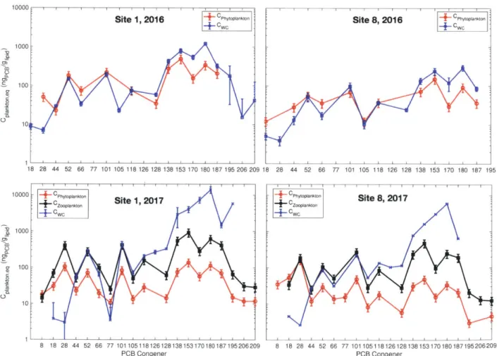
In Figure 5, the concentrations of PCBs in measured and estimated from water column plankton from site 1 and site 8 in 2016 and 2017. The water column data was obtained by applying the lipid-water partition constant to the data in Fig. 4. For clarity, only the estimates for water column data are shown since they are similar to the 0-5 cm data.
For the purposes of this study, the concentrations of four abundant congeners measured in the phytoplankton are focused on: PCB 52 (4-Cl), PCB 101 (5-Cl), PCB 153 (6-Cl) and PCB 180 (7-Cl). Of these four congeners, two coelute with other PCBs. PCB 52 coelutes with congener PCB 43. PCB 43 is abundant in lower chlorinated Aroclor mixtures which are not expected to be seen in Lake Cochituate. PCB 153 is the congener of most abundant mass. Although it has a small shoulder coelution with PCB 132, it presents in 3:1 predominance over congener 132 in Aroclor mixtures 1254 or 1260.
For the extract concentrations, the calibration curve measures of specific congeners showed a
- 0-5cm
A-phytoplankton concentrations would be 25% given uncertainties in TS values and volumes extracted. Measured extract volumes were small (16-122 pl), but they were calculated with 4-12% precision (Table S14). Measured concentrations were surrogate recovery corrected with their chlorine number equivalent congener. The average 4-7 Cl surrogate recoveries for the 2016 phytoplankton were between 75-118%, with corresponding RSD 14-7% (Table S14). The 2017 phytoplankton recoveries ranged 47-86% with corresponding RSD 6-10%. The zooplankton recoveries were 83-99% with corresponding RSD 10-15%. Average RSDs between 6-15%
suggest that the extracts processed together were handled similarly, even when volumes were different.
The relationship between congeners from each 2016 phytoplankton, 2017 phytoplankton and 2017 zooplankton sample are consistent with that of a mixed Aroclor signature. In Aroclor 1260, the relative abundances of PCB 101, PCB 138 and PCB 187. PCB 52 are 5, 6 and 4%,
respectively [36]. There is no contribution to PCB 52 in Aroclor 1260. PCB 52 is present in Aroclor 1242 and 1354 at 4 and 5%, respectively. Apell et al. reports a theoretical concentration of an Aroclor mixture contain 37% Aroclor 1254 and 63% Aroclor 1260 [3].
Figure 4 Concentration of PCBs in plankton and estimated from truly dissolved water column data obtained using passive samplers.
10000 1000 CD, 0 M 100 10~ 10000 CO 0 CL, 0 1000 100 10 8 18 28 44 52 66 77 101105118126128138153170180187195206209 PCB Congener Site 8, 2016 12 3 137 op8ankion 18 28 44 52 66 77 101 105 118 126 128 138 153 170 180 187 195 8 18 28 44 52 66 77 101105118126128138153170180187195206209 PCB Congener Site 1, 2016 4 Ch,nkn + cwec 18 28 44 52 66 77 101 105 118 126 128 138 153 170 180 187 195 206 2M Cehytopiankion Zooplankton 1,2017 4- CWC PhyCoplankto" Site 8, 2017 cZooplankton +CWC 1