A block-tridiagonal solver with two-level
parallelization for finite element-spectral codes
The MIT Faculty has made this article openly available.
Please share
how this access benefits you. Your story matters.
Citation
Lee, Jungpyo and Wright, John C. “A Block-Tridiagonal Solver with
Two-Level Parallelization for Finite Element-Spectral Codes.”
Computer Physics Communications 185, 10 (October 2014): 2598–
2608 © 2014 Elsevier B.V.
As Published
http://dx.doi.org/10.1016/j.cpc.2014.06.006
Publisher
Elsevier
Version
Author's final manuscript
Citable link
http://hdl.handle.net/1721.1/113076
Terms of Use
Creative Commons Attribution-NonCommercial-NoDerivs License
A block-‐tridiagonal solver with two-‐level parallelization for finite
element-‐spectral codes
Jungpyo Lee
Massachusetts Institute of Technology (MIT), Cambridge, MA John C. Wright
Massachusetts Institute of Technology (MIT), Cambridge, MA
Abstract:
Two-‐level parallelization is introduced to solve a massive block-‐tridiagonal matrix system. One-‐level is used for distributing blocks whose size is as large as the number of block rows due to the spectral basis, and the other level is used for parallelizing in the block row dimension. The purpose of the added parallelization dimension is to retard the saturation of the scaling due to communication overhead and inefficiencies in the single-‐level parallelization only distributing blocks. As a technique for parallelizing the tridiagonal matrix, the combined method of “Partitioned Thomas method” and “Cyclic Odd-‐Even Reduction” is implemented in an MPI-‐Fortran90 based finite element-‐spectral code (TORIC) that calculates the propagation of electromagnetic waves in a tokamak. The two-‐level parallel solver using thousands of processors shows more than 5 times improved computation speed with the optimized processor grid compared to the single-‐level parallel solver under the same conditions. Three-‐ dimensional RF field reconstructions in a tokamak are shown as examples of the physics simulations that have been enabled by this algorithmic advance.
Key Words: Two-‐level parallel computing, block tridiagonal solver, partitioned Thomas method, cyclic odd-‐even reduction, plasma waves
PACS: 52.35.Hr, 52.65.-‐y
Author’s addresses: Jungpyo Lee, Plasma Science and Fusion Center, Massachusetts Institute of Technology (MIT), Cambridge, MA, USA, [email protected]; John C. Wright, Plasma Science and Fusion Center, Massachusetts Institute of Technology (MIT), Cambridge, MA, USA, [email protected]
1. Introduction
The numerical solution of partial differential equations in two dimensions often produces a block-‐ tridiagonal matrix system. This tridiagonal structure generally appears by the discretization along one coordinate in which only adjacent mesh points or elements are coupled. If the coupling along the second dimension is in a local basis, the resulting blocks can be sparse or banded. When a global basis is used (e.g. Fourier spectral basis), the size of the blocks may be comparable to the number of block rows and each block can be massive. For larger problems, in-‐core memory may not be sufficient to hold even a few blocks, and so the blocks must be distributed across several cores. Thus, the parallelization of the solver for the “massive block”-‐tridiagonal system is required for not only the scaling of the computation speed but also the distribution of the memory.
The electromagnetic wave code (TORIC) [1] is an example of a system producing a “massive block”-‐tridiagonal matrix that solves Maxwell’s equations and calculates the wave propagation and damping [2-‐4] which are important in magnetic confinement fusion research. We have shown in previous work [5] that significantly improved performance is achieved in solving this block-‐tridiagonal system by introducing parallelism along the block rows in addition to within the dense blocks. In this article, we explain in detail this two-‐level parallelization of the solver using a three-‐dimensional (3-‐D) processor configuration and how operation counts and parallel saturation effects in different parts of the algorithm explain the efficient scaling of the computation speed that has been observed.
The TORIC code is written in MPI-‐Fortran90, and uses the spectral collocation and finite element methods (FEM) to solve Maxwell’s equations in Galerkin’s weak variational form,
dV F∗ ∙ −!! !!∇×∇×E + E + !"! ! (J!+ J!) = 0, (1)
where 𝑐 is the speed of light in a vacuum, E is the electric field, J! is the plasma current response to the electric field, J! is the applied antenna current, 𝜔 is the prescribed frequency of the applied antenna current, and dV is the differential volume. Here, F is a vector function in the space spanned by the basis of E, satisfying the same boundary condition as E. Equation (1) is solved for three components of the electric field vector (radial, poloidal and toroidal direction) and their radial derivatives. The radial dimension is discretized by finite elements expressed in the cubic Hermite polynomial basis1, and the
poloidal and toroidal dimensions use a Fourier spectral basis [1, 5], as shown in E(𝑟, 𝜙, 𝜃) = !! E!,!(𝑟)𝑒!(!"!!") !!!!! !! !!!!! , (2)
where 𝑟 is the radial coordinate, 𝜙 and 𝜃 are the toroidal and poloidal angle, 𝑛 and 𝑚 are the toroidal and poloidal spectral modes, and 𝑙! and 𝑙! are the maximum toroidal and poloidal mode numbers considered, respectively.
While the toroidal spectral modes are decoupled due to the toroidal axisymmetry of a tokamak, the poloidal spectral modes are coupled by the dependence of the static magnetic field on the poloidal
angle. For a fixed toroidal spectral mode, the wave equation in Eq. (1) reduces to a two-‐dimensional (2-‐ D) problem (radial and poloidal). The constitutive relation between the plasma current and the electric field for each poloidal mode (m) at a radial position (r) is given by
J!!,! 𝑟 = −!"!!𝜒 ∙ E!,!(𝑟), (3)
where 𝜒(𝜔, 𝑛, 𝑚) is the susceptibility tensor that is anisotropic in the directions parallel and perpendicular to the static magnetic field (see [1, 2] for the derivations of 𝜒). Here, the electric field, E!,!(𝑟), is radially discretized by n
! finite elements (i.e. 𝑟 = 𝑟! where the index of the elements are 𝑖 = 1,∙∙∙, n!).
Using Eqns. (2-‐3) and the given boundary condition for J!, Eq. (1) results in a master matrix that has a radial dimension of n! block rows, and each row has three blocks, L!, D! and R! due to the adjacent radial mesh interactions that are introduced through the cubic Hermite polynomial basis set of the FEM representation. The size of each block is n!×n!, and contains the poloidal Fourier spectral information. The dimension n! is equal to six times the poloidal spectral mode number (i.e. n!= 6(2𝑙!+ 1)), where the factor of six is from the three components of the electric field and their derivatives. The discrete block-‐tridiagonal system form of Eq. (1) consists of the matrix equation,
L!∙ x!!!+ D!∙ x!+ R!∙ x!!! = y! for i=1,… n!, (4)
where each x! and y! is a complex vector, every element in L! and R!! is zero, and y! is determined by
boundary conditions. The total master matrix size is (n!n!)×(n!n!), with typical values of n! and n! for a small size problem being about 200 and 1000 respectively (see Fig. 1).
Many methods have been investigated to parallelize the solution of this block-‐tridiagonal system by considering it as either just a “tridiagonal” system [6-‐9] or a “block” matrix system [10]. The “tridiagonal” system is parallelized in the block row dimension, and the “block” matrix system is
parallelized by distributing the blocks. In other words, in some cases the parallel algorithm for a block tridiagonal system is adopted in which the rows of the master matrix are divided among a one-‐ dimensional (1-‐D) processor grid and they are calculated with a “cyclic reduction method” [6] or
“partitioned Thomas method” [7-‐8] as in the simple tridiagonal problem. The “cyclic reduction method”
of solution uses the simultaneous odd row elimination with logarithmic recursive steps, O(log(n!)), “partitioned Thomas method” requires O(n!/p!) elimination steps in divided groups (see Table 1). The “block” matrix system approach keeps the serial routine of the Thomas algorithm [11], and, for each block operation, use a parallelized matrix computation algorithm such as ScaLAPACK [12] in a two-‐ dimensional (2-‐D) processor grid.
These two parallelization methods have different scaling and saturation characteristics at large number of processors. Combining the methods for two-‐level parallelization in a three-‐dimensional (3-‐D) processor grid overcomes their saturation limitations and achieves better scaling. This dual scalability by two-‐level parallelization has also been used in a solver [13] that employs a cyclic reduction method for parallelizing block rows and multithreaded routines (OpenMP, GotoBLAS) for manipulating blocks. This BCYCLIC solver [13] and our solver have similar features of algorithmic advantage for efficient dual
scaling as will be shown in Fig. 2, while they are suitable for application to different sizes of block-‐ tridiagonal systems since they have different memory management. In particular, the BCYCLIC solver is efficient for systems where several block rows can be stored in a single node for multithreaded block operations, while our solver does not have a limitation on the use of out-‐of-‐core memory or multiple nodes for splitting large block sizes that cannot be stored in the core memory of a single node, since it uses ScaLAPACK instead of LAPACK/BLACS with threads used in [13]. The block size of TORIC is typically too large to store several block rows in a node because of the global spectral basis.
A single-‐level parallel solver in TORIC was implemented with the serial Thomas algorithm along the block rows and 2-‐D parallel operations for the blocks [14]. ScaLAPACK (using routines: PZGEMM, PZGEADD, PZGETRS, PZGETRF) [12] was used for all matrix operations including the generalized matrix algebra of the Thomas algorithm. All elements in each block are distributed in the uniform 2-‐D processor grid whose dimension sizes are the most similar integers to each other. For efficient communication, the logical block size used by ScaLAPACK is set by b×b and so the number of processors (P!"!) is constrained to be less than (n!/b)!. A small logical block size may be chosen to increase the number of processors available for use at the cost of increased communication (e.g. b ≃ 72). We have found through experimentation that communication degrades performance even as this constraint is approached. Only when (n!/b)! is much larger than P!"!, this single-‐level solver implementation is efficient.
This limitation on the number of processors that can be used efficiently with the single-‐level solver may present load balancing problems and result in many idle processors in a large, integrated multi-‐ component simulation such as those carried out in the CSWIM Fusion Simulation Project [15] and the transport analysis code TRANSP [16]. For a relatively small problem, n!= 270 and n! = 1530 with 20 processors, the completion time to run TORIC is about one hour. Our purpose is to reduce this time to the order of minutes by the use of about 1000 processors through improved scaling. We will demonstrate that the two-‐level parallel solver using 3-‐D processor configuration within the dense blocks (2-‐D) and along the block rows (1-‐D) can achieve good scaling for small and large problems.
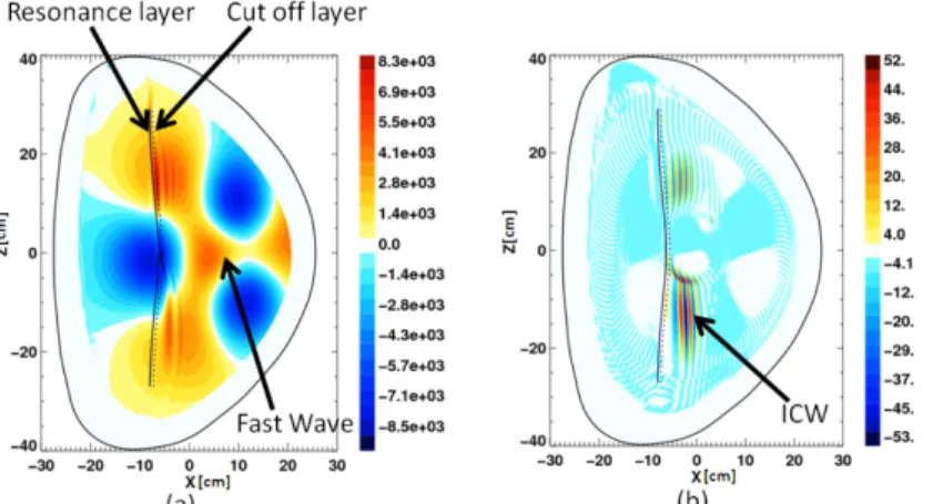
The plan of this paper is as follows: In Sec. 2, we compare the characteristics of several algorithms for parallelization along the block rows. According to our semi-‐empirical model, the combined algorithm of the partitioned Thomas method and cyclic reduction, which was developed in [9], is selected for our solver because of the efficient dual scalability and stability. In Sec. 3, the implementation of the combined algorithm as the two-‐level parallel solver is explained, and in Sec 4, we present test results of the computation speed for the two-‐level parallel solver and compare it with the single-‐level parallel solver. We also discuss accuracy, stability and memory management of the solver. Section 5 introduces two examples for a physics problem to which the two-‐level parallel solver can be applied: three-‐ dimensional (in space) wave field simulations in the ion cyclotron range of frequencies (ICRF) and the lower hybrid range of frequencies (LHRF). The two-‐level parallel solver makes these computationally intense problems feasible to solve. Conclusions of this paper are given in Sec 6.
Figure 1. A schematic of the two-‐level parallelization using 3-‐D processor configuration for a block-‐tridiagonal system. The size of each block, L, D and R is n!×n! and there are n! rows of the blocks. The rows are divided into P! groups, and the
elements of each block are assigned to P!P! processors. Thus, every element has a 3-‐dimensional index corresponding to the
assigned processor among the total number of processors, P!"!= P!P!P!.
2. Selection of the parallel algorithm
To select a parallel algorithm along the block rows adequate for the two-‐level parallel solver, we compared the matrix operation count and the required memory for the algorithms typically used for block-‐tridiagonal matrix solvers in Table 1. The common parallel block-‐tridiagonal solvers use a single-‐ level parallelization using 1-‐D processor grid (i.e. P!"!= P!), because the algorithm, whether it is Partitioned Thomas method [7] or odd-‐even cyclic reduction [6], is easily applicable to a 1-‐D processor grid, and the usual block size n! is much smaller than the number of blocks n!. However, for the massive block system such as produced with the coupled FEM-‐Spectral method, n! is as big as n!. Storing several blocks each of size n!×n! using in-‐core memory would be impossible for such a massive system. Thus
we parallelize each block as well, giving the two-‐level parallelization for the required memory and desired calculation speed.
If the block operation time is ideally reduced by the number of processors used in the operation, it is always most efficient in terms of number of floating point operations and memory to use the Thomas algorithm with a serial calculation in rows and parallelized block operations on the 2-‐D processor grid (i.e. P!"!= P!P!). However, the additional operation for the parallelization and the increased communication between the processors deteriorate the improvement in speed from parallelization as the number of processors increases and becomes comparable to the square root of the size of a block divided by the logical block size (e.g. P!"!~(n!/72)!). Also, beyond this limit, additional processors have no work to do and remain idle. A good way to avoid both memory and speed problems and retain full utilization of processors is to add another dimension for the parallelization, so the total processor grid configuration becomes three dimensional (i.e. P!"!= P!P!P!) in the two-‐level parallelization.
The partitioned Thomas method uses a “divide and conquer” technique. The system (master matrix) is partitioned into P! subsystem, which proceeds with eliminations by the Thomas method simultaneously and results in “fill-‐in” blocks. The “fill-‐in” blocks are managed to find a solution through the communications between the subsystems [7]. Conversely, the cyclic odd-‐even reduction algorithm [6] has no matrix fill-‐in step that requires significant additional time in the partitioned Thomas method. The logarithmic cyclic reductions of the algorithm are the most efficient when both P! and n! is approximately a power of 2. When either P! or n! is not a power of 2, the cyclic algorithm is still available by modifying the distribution of processors and communicating each other as shown in [13]. For “massive block”-‐tridiagonal system, P! is typically assigned to be less than n!/2 to treat the massive blocks using some processors of P!P!. When P! is assigned to be less than n!/2, it induces n!/2P!+ n!/4P!+. . . +2 = n!/P!− 2 additional series of operation to the logarithmic reduction process in the cyclic reduction algorithm (see the first row of Table 1).
The combined algorithm of the partitioned Thomas method and the cyclic reduction was introduced in [9]. This combined algorithm was used in this case for the analysis of a solar tachocline problem to enhance both the speed and the stability of the calculation. It can alleviate the local pivoting instability problem of the cyclic reduction method because it is based on the partitioned Thomas method except that it uses cyclic reduction for dealing with the matrix fill-‐in and for communication between the 𝑃! groups. The computation time for the fill-‐in reduction process of the partitioned Thomas method [7], 𝑃!(𝑀 + 𝐴 + 2𝐷), is replaced by the term from the cyclic reduction algorithm [6] in the combined algorithm, (log!𝑃!− 1)×(6𝑀 + 2𝐴 + 𝐷) (see table 1). Here M, A, and D are the computation time for block multiplication, addition, and division respectively. The contribution of this paper is a generalization of the work in [9] to include parallelization of the block operations and to characterize the performance properties of the resulting two-‐level parallelization.
We have developed an execution time model for the block operations, 𝑀, 𝐴 , and 𝐷 including the saturation effect in Eqn. (5)-‐(7), in order to compare the realistic speed of the algorithms. From the observation that the deterioration of scaling by parallelization in 𝑃!𝑃! becomes severe as the number of processors approaches the saturation point, we set the exponential model in Eq. (8) as:
𝑀 = 𝑀! !! ! !!!! !"" (5) 𝐴 = 𝐴! !! ! !!!! !"" (6) 𝐷 = 𝐷! !! ! !!!! !"" (7) 𝑃!𝑃! !"" = 𝑃!𝑃! !"#∗ 1 − exp − !!!!! !!! !"# !(!!!!) (8)
The exponent parameter, 𝛼(!!!!), represents the non-‐ideal scaling because 𝑃!𝑃! !"" becomes
about 𝑃!𝑃! !(!!!!) when 𝑃!𝑃! is much smaller than 𝑃!𝑃! !"#. Ideally, 𝛼(!!!!) should be 1. However,
from actual tests of the run time in section 4, we can specify the parameters, 𝛼(!!!!) = 0.41 and
𝑃!𝑃! !"# = 𝑛!/191 ! from Fig 4-‐(a). These constants may not be generally true for all range of processor and for all architectures, but it can explain the results well in our test shown in Fig. 4. Also, we set the parameters, 𝑀!= 0.5𝐷!= 𝑛!𝐴!, because the general speed of matrix multiplication in a well optimized computation code is about two times faster than that of matrix division based on experience when the matrix size is about 1000×1000.
No communication saturation model is used for the 𝑃! decomposition in this comparison. For cyclic reduction steps in the first and third row of Table 1, they have a natural algorithmic saturation from the log!𝑃! term that dominates over any communication saturation. Unlike the distribution of a matrix block among 𝑃!𝑃! processors, increase of 𝑃! does not fragment matrix block among more processors but has the weaker effect of increasing communication boundaries between block row groups. Additionally, for the massive block system, we typically use 𝑃!≪ 𝑛! in which there is little saturation in the parallelization due to the communication.
The computation time per processor is estimated for the algorithms in Fig. 2 for a relatively small size system problem, n!= 270 and n!= 1530. Both the combined algorithm and the cyclic reduction algorithm show the similar performance of the two-‐level scaling and they have typically smaller computation time than the partitioned Thomas algorithm. This model is demonstrated by the real computation results in Fig. 6 that agree well with the models in Fig. 2 (compare the blue asterisk and the black curve in Fig. 2 with Fig. 6). Among the algorithms, we selected the combined algorithm because it is known to be more stable than the original cyclic reduction algorithm [9]. Some stability issues of the original cyclic reduction were also fixed in the Buneman version of cyclic reduction with a reordering of operations [17-‐19].
Computation time per processor
Maximum memory in a processor[unit of complex data format] Cyclic Odd-‐Even Reduction Algorithm [6,13] (log!𝑃2!+ (𝑛𝑃! !− 2))×(6𝑀 + 2𝐴 + 𝐷) 𝑛! 𝑃! (2𝑛!!+ 2𝑛!) 𝑃!𝑃! Partitioned Thomas Algorithm [7] 𝑛! 𝑃! 4𝑀 + 2𝐴 + 2𝐷 + 𝑃!(𝑀 + 𝐴 + 2𝐷) 𝑛! 𝑃! (2𝑛!!+ 2𝑛!) 𝑃!𝑃! Combined Algorithm [9] 𝑛! 𝑃! 4𝑀 + 2𝐴 + 2𝐷 + log! 𝑃! 2 ×(6𝑀 + 2𝐴 + 𝐷) 𝑛! 𝑃! (2𝑛!!+ 2𝑛!) 𝑃!𝑃!
Serial Thomas Algorithm (𝑃!= 1) [20]
𝑛!(𝑀 + 𝐴 + 𝐷) 𝑛!(𝑛!!+ 2𝑛!)/𝑃!𝑃!
Table 1. Comparison of the parallel algorithms for block-‐tridiagonal matrix with 𝑛! block rows where each block is size n!×n!. The total number of processors P!"!= P!P!P!, 𝑛!is parallelized in P! groups and each block in a group is parallelized on the P!P! processor. Here, 𝑀, 𝐴, and 𝐷 are the computation time for block multiplication, addition, and division, respectively, which can be modeled in Eqn. (5)-‐(7).
Figure 2. Estimation of the computation time per processor based on Table 1 for n!= 270 and n!= 1530. The time for two-‐level parallel algorithms (cyclic odd-‐even reduction, partitioned Thomas method, and combined
1
10
0
5
10
computation time per processor [A.U.]
p
tot=64
P
2P
31
10
100
0
5
10
p
tot=128
P
2P
31
10
100
0
5
10
P
2P
3p
tot=256
1
10
100
0
5
10
P
2P
3p
tot=512
Cyclic reduction Partition Thomas Combined method Serial Thomas (P 2P3=Ptot)method) is estimated in terms of P!P! for various P!"!, and the time for the single-‐level parallel algorithm (serial Thomas) is marked as an asterisk at P!P!= P!"!. The saturation effects are included by the model in Eqn. (5)-‐(7) for 𝑀, 𝐴, and 𝐷.
3. Code Implementations
One approach for implementing the 3-‐D grid for the two-‐level solver is to use a context array in BLACS [21], in which each context uses the 2-‐D processor grid as does the single-‐level solver [12]. In BLACS, a context indicates a group within a boundary of an MPI communicator. Under the default context having the total number of processors, it is possible to assign multiple sub-‐contexts (groups) by mapping each processor. Also, we can communicate across sub-‐contexts when needed in a tridiagonal algorithm.
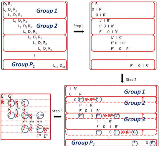
The combined algorithms of partitioned Thomas method and cyclic odd-‐even reduction [9] can be summarized as three forward reduction steps and two back substitution steps. By partitioning the whole system into 𝑃! groups and applying the Thomas algorithm in each group, we can achieve a subsystem containing 𝑃! rows to be communicated across the groups using the cyclic reduction. Once we achieve the solution for a row after the cyclic reduction, the solution is substituted to find another row solution within the subsystem, and then finally substituted backward as in the Thomas algorithm for each group.
3.1. Divided forward elimination and Odd-‐even cyclic reductions
The three forward steps are described in Fig. 3. The first step is for serial elimination of the L! block by the previous row (i-‐1th row) as in the Thomas algorithm, but this process is executed
simultaneously in every group like a typical partition method. During the first step, the elimination processes create the fill-‐in blocks “F’” at the last non-‐zero column of the previous group except for the first group (see Fig. 3-‐step 1).
Step 2 is the preliminary process for step 3, the cyclic reduction step which requires tridiagonal form. To construct the upper level tridiagonal form composed of the circled blocks in the first row of each group (see Fig. 3-‐step 2), we need to move the blocks G’’ in the first row to the column where the block E’’ of the next group is located. Before carrying out the redistribution, the matrices in the last row in each group must be transmitted to the next group. Then, the received right block R’ is eliminated by the appropriate linear operation with the following row, and the elimination by the next row is repeated until the block G’’ moves into the desired position.
The block tridiagonal system formed by the E’’, F’’ and G’’ blocks from each processor group can be reduced by a typical odd-‐even cyclic reduction in step 3 as shown in Fig. 3. This step is for the communication of information between groups, so the portion of the total run time for this step is increased as 𝑃! is increased. This reduction is carried out in log!((𝑃!+ 1)/2) steps because 𝑃! should be 2!− 1 instead of 2! where 𝑛 is an integer, and it requires the total number of processors to be several times (2!− 1) (i.e. 𝑃
!"! = 𝑃!𝑃!(2!− 1)). This characteristic could be a weak point of this algorithm in a practical computation environment, because a node in a cluster consists of 2! processors typically. However, the problem can be solved by assigning (2!− 1) nodes that have 𝑚 processors in a node, which results in no free processor on certain nodes and has minimal communication across the nodes.
Figure 3. Description of the combined algorithm for the forward elimination (Step 1), the block redistribution (Step 2), and the cyclic odd-‐even reduction (Step 3).
3.2. Cyclic substitutions and divided backward substitutions
In the end of the cyclic reduction in step 3 only one block E’’’ remains, so we can obtain a part of the full solution by taking x!= E′′′!!y!. This part of the solution is substituted to find a full solution vector, x, in step 4 and step 5. In step 4, the cyclic back substitution is executed in log!((𝑃!+ 1)/2) steps, the same as in the cyclic reduction step. Then, in each group, the serial back substitution continues simultaneously in step 5. In this step, each group P! except the first one should have the information of the solution in the previous group P!!! to evaluate the terms contributed by the fill-‐in blocks F’’ in the solution.
4. Result and Discussions
4.1. Computation speed of the solver
The computation speed of the solver using the combined algorithm is evaluated with various 3-‐D processor grids, [P!, P!, P!], for three different size problems as shown in Fig. 4. Each graph shows the result for different decompositions of the processor grid. The red line indicates the single-‐level solver scaling which saturates due to large communication time well before the number of processors is comparable to (n!/72)!, which is the ratio of block size to the logical block size of ScaLAPACK. However, the graphs for the two-‐level solver show fairly good and stable scaling. For the large number of processors in Fig. 4-‐(c), the two-‐level solver with an optimized configuration is about 10 times faster than the single-‐level solver. This test for wall-‐clock time was conducted on the massively parallel Franklin computing system at the National Energy Research Scientific Computing Center (NERSC). Each of Franklin's compute nodes consists of a 2.3 GHz quad-‐core AMD Opteron processor (Budapest) with a theoretical peak performance of 9.2 GFlop/sec per core. Each core has 2GB of memory.
In the log-‐log graph of run time as a function of the number of processors, an ideal scaling from parallelization has a slope of -‐1. Although the ideal scaling is hard to achieve because of increasing communication, the two-‐level solver shows a much steeper slope than the single-‐level solver. We can consider the slope as the average efficiency of the scaling. For the small size problem in Fig 4-‐(a), we evaluate the speed-‐up2 (= T(P
!"#)×P!"#/T(P!"!)) by selecting the reference point as the first point (P!"# =8) of the single-‐level solver. For example, the two-‐level solver with P!P!=16 (magenta line with plus symbols, slope=-‐0.55) shows that the speed-‐up by the different total number of processors (P!"!= 16, 48, 112, 240, 496, 1008, 2032) are respectively 10.4, 12.1, 24.6, 43.7, 64.3, 84.6, and 120.1. Their corresponding efficiencies (= T(P!"#)×P!"#/(T(P!"!)×P!"!)) are 65, 25, 22, 18, 12, 8.4, and 5.9%. For the medium size problem in Fig 4-‐(b), using the first point (P!"# =64) of the single-‐level solver (red line) for the reference point, the speed-‐up of the two-‐level solver with P!P!=16 (light blue line with diamond symbols, slope=-‐0.70) by the different total number of processors (P!"!= 112, 240, 496, 1008, 2032) are 69.0, 138.2, 250.2, 381.6, and 522.0. Their corresponding efficiencies are 61, 57, 50, 37, and 25%. We note for the cases in Fig. 4-‐(a) and 4-‐(b) the processor number and speed-‐up are comparable to those in [13] (see Fig. 4 in [13]). For the large size problem in Fig 4-‐(c), we may use the first point (P!"#=1920) of the two-‐level solver with P!P!=128 for the reference point, because the single-‐level solver (red line) shows saturation of the scaling already at this point. Then, the speedup of the two-‐level solver with P!P!=128 (green line with cross symbols, slope=-‐0.79) by the different total number of processors (P!"!= 3968, 8064, and 16256) are 3498, 6508, and 10160. Their corresponding efficiencies of the scaling are 88%, 80%, and 60%, respectively. As the results are represented as lines on a log-‐log graph, the efficiencies based on the linear speed-‐up decrease with increasing number of processors.
The non-‐ideal scaling parameters for P!P! used in the model of section 2 can be inferred from the red graph in Fig. 4-‐(a) in which all processors are used for the parallelization in blocks (P!"!= P!P!). The
2 A serial solver using a processor (P
!"# =1) is an ideal reference point for the scaling by the parallelization. However, in this test, the reference point P!"#> 1 is used due to the constraint of the required memory for the massive system.
exponent parameter, 𝛼(!!!!)= 0.41, is obtained by the average slope in the log-‐log graph before the
saturation point. The saturation point for n! = 1530 is around P!P!= 64 where the graph begins to be flat, giving the parameter 𝑃!𝑃! !"# = 𝑛!/191 ! . The red graphs in Fig. 4-‐(b) and (c) showing the full saturations beyond P!P!= 256 and beyond P!P!= 1024, respectively, are also consistent with the saturation points in Fig. 4-‐(a). For the two-‐level parallel solver using 3-‐D processor grid shows
retardation of the saturation because P! can be used to make P!P! less than 𝑃!𝑃! !"#. Also, as shown in Fig. 4-‐(a)(b) and (c), the slopes become generally steeper for the larger size problem or for smaller processor number, as they are far from the saturation point. These facts validate the exponential form of the model used in section 2.
Figure 5 shows the allocated computation time for the steps of the combined algorithm within the run time of the two-‐level solver. As the number of groups P! is increased at a fixed number of block rows n!, the dominant time usage is shifted from step 1 and 2 to step 3 in Fig. 3 due to fewer partitioned blocks per group and more cyclic reductions. The graphs in Fig. 5 are in accordance with the expected theoretical operation of the combined algorithm in section 2. Since the operation count of the partitioned Thomas part in the step 1 and step 2 is proportional to n!/P!, the slope is about -‐1. But the cyclic reduction part in step 3 results in a logarithmic increase of the graph because the operation count is proportional to log!P!, as indicated in Table 1. For large P! with a fixed P!P! , the run time of step 3 is dominant component of the total run time, which implies the algorithmic saturation of the parallelization in P!. This algorithmic saturation is shown in the reduced slope of the black line in Fig. 4-‐ (a) when log!P!≥ n!/P!. Note that the flat slope of all graphs except the red graph in Fig. 4-‐(a) when P!> n!/2 is not due to the algorithmic saturation but due to the constraint of the parallelization by P!≤ n!/2.
An enhanced improvement in speed-‐up relative to ideal scaling (i.e. the steeper slope than -‐1) is seen in Fig. 5 for step 2 for large P!. The reason for this could be specific to the algorithm, i.e. the matrix operations of the first row in each group are much smaller than for the rest of the rows in the group, and some of the remaining rows become the first rows in a group as we divide into more groups with increased P!.
This saturation of the single-‐level parallelization either in P! or in P!P! implies the existence of an optimal 3-‐D processor configuration for the two-‐level parallelization. We found that the optimal 3-‐D grid exists at the minimum total run time when P!P!≈ 16 for n!= 1530 and n!= 3066, and P!P! ≈ 128 for n!= 6138, provided the number of processors is big enough. Figure 6 shows the run time comparison in terms of P!P! for n!= 1530. As mentioned in section 2, the results of Fig. 6 are reasonably consistent with the non-‐ideal scaling model we developed for the algorithm comparison. Thus, the optimal grid for the minimal computation time can be estimated from the modeling in section 2 without the full test such shown in Fig. 6.
It is important to point out that the two-‐level parallel solver is not always faster than the single-‐ level parallel solver because the serial Thomas algorithm has fewer matrix operations and thus works well with a small number of processors far before the saturation point. For example, the single-‐level solver shows the faster computation speed than any 3-‐D configuration of two-‐level solver below P!"! =32 in Fig. 4-‐(a).
From Table 2 obtained by the IPM monitoring tool [22] at NERSC, we can compare the saturation effect from MPI communication for the two solvers. Although this tool does not measure the communication time in a specific subroutine, it does monitor the total run time including pre-‐processing and post-‐processing, and we can see a remarkable difference between the single-‐level parallel solver and the two-‐level parallel solver. As the total number of processors ( P!"!) is increased, MPI communication time increases at a much faster rate for the single-‐level solver than it does for the two-‐ level solver. When P!"! changes from 32 to 2048, the ratio of the communication time to the total run time increases about three times for single-‐level solver, while the ratio for the two-‐level solver increases only about two times. Also, the drop of the average floating point operation speed (Gflop/s) in terms of the total core number for the single-‐level solver is more severe than the speed drop-‐off for the two-‐level solver. Both of these observations demonstrate the retarded saturation that can be credited for the reduced communication of the two-‐level solver.
In the second column of Table 2, even before the saturation point (e.g. P!"!= 32), we can see about 3 times higher average execution speed for the two-‐level solver than for the single-‐level solver (compare Table 2-‐(a) with (d)). This is also a significant benefit of the use of the two-‐level solver. The difference of the execution speed may depend on the efficiency of the calculation by ScaLAPACK in a given block size with a different number of processors (note that the single-‐level solver uses all cores whereas the two-‐level solver uses the fraction P!P!/P!"! of cores for the ScaLAPACK operations). Hence, the two-‐level solver algorithm has more efficient data processing (e.g. fewer cache misses and calculation in a larger loop) as well as less communication overhead. Furthermore, from Table 2-‐(e) and (f), we can see that the scaling by ScaLAPACK is less efficient than that by the combined algorithm along the block rows.
(a) (b) 101 102 103 102 103 number of processors Execution time(sec) n1=270, n2=1530 slope*=−0.41 slope=−0.55 slope* =−0.43 2D(Thomas) P tot=P2P3 1D(combined) P 1~Ptot/1; P2P3=1 3D(combined) P1~Ptot/2; P2P3=2 3D(combined) P 1~Ptot/4; P2P3=4 3D(combined) P 1~Ptot/8; P2P3=8 3D(combined) P 1~Ptot/16; P2P3=16 102 103 102 103 104 number of processors Execution time(sec) n 1=480, n2=3066 slope=−0.12 slope=−0.31 slope=−0.53 slope=−0.70 slope=−0.70 2D(Thomas) P tot=P2P3 3D(combined) P1~Ptot/4; P2P3=4 3D(combined) P1~Ptot/8; P2P3=8 3D(combined) P1~Ptot/16; P2P3=16 3D(combined) P 1~Ptot/32; P2P3=32
(c)
Figure 4-‐(a)(b)(c). Comparison of the solver run time in terms of various 3-‐D processor grid configurations [𝐏𝟏, 𝐏𝟐, 𝐏𝟑] with
different size problem (a) [𝐧𝟏, 𝐧𝟐] = 𝟐𝟕𝟎, 𝟏𝟓𝟑𝟎 , (b) [𝐧𝟏, 𝐧𝟐] = 𝟒𝟖𝟎, 𝟑𝟎𝟔𝟔 , and (c) [𝐧𝟏, 𝐧𝟐] = 𝟗𝟖𝟎, 𝟔𝟏𝟑𝟖 . The red
graph corresponds to the single-‐level parallel solver that uses of the serial Thomas algorithm along the block rows and 2-‐D parallel operations for blocks. The other graphs (blue, green, cyan, and black) correspond to the two-‐level solver that uses 1-‐ D parallelization by the combined algorithm in Section 2 along block rows and uses 2-‐D parallel operations for blocks. The slope values next to the lines indicate the average of the slopes of the graphs, and the “slope*” indicates the average slope before the saturation point.
103 104 103 104 number of processors Execution time(sec) n1=980, n2=6138 slope=0.02 slope=−0.84 slope=−0.79 slope=−0.52 slope=−0.88 2D(Thomas) P tot=P2P3 3D(combined) P 1~Ptot/32; P2P3=32 3D(combined) P 1~Ptot/128; P2P3=128 3D(combined) P 1~Ptot/256; P2P3=256 3D(combined) P 1~Ptot/512; P2P3=512
Figure 5. Run time of the forward reduction steps in the two-‐level solver with a small size problem [n!, n!] = 270,1530.
Step 1 is a divided forward elimination process. Step 2 is a preliminary process for making the tridiagonal form needed for Step 3, which is a typical cyclic odd-‐even reduction process. The step 3 shows the logarithmic increase as indicated in Table 1. The summation of the three run times of step 1,2, and 3 corresponds to the yellow graph with triangle symbols in Fig. 4-‐(a)
Figure 6. Comparison of the solver run time in terms of 𝐏𝟐𝐏𝟑 with a small size problem [𝐧𝟏, 𝐧𝟐] = 𝟐𝟕𝟎, 𝟏𝟓𝟑𝟎 . Compare this
result with the estimation for the combined algorithm (black line) and Thomas algorithm (blue asterisk) in Fig. 2. 1 10 0 200 400 P 2P3 P tot=64 1 10 100 0 200 400 P 2P3 Ptot=128 1 10 100 0 200 400 P2P3
Computation time per processor (sec)
Ptot=256 1 10 100 0 200 400 P2P3 Ptot=512 3D (Combined method) 2D (Thomas P 2P3=Ptot)
%comm gflop/sec gbyte
(a) Single-‐level solver (ptot=p2p3=32) 26.2 0.719 0.522 (b) Single-‐level solver (ptot=p2p3=128) 38.4 0.438 0.292 (c) Single-‐level solver (ptot=p2p3=2048) 78.1 0.110 0.188 (d) Two-‐level solver (ptot=32,p2p3=1) 34.6 2.596 1.486 (e) Two-‐level solver (ptot=128,p2p3=1) 53.5 1.714 1.051 (f) Two-‐level solver (ptot=128,p2p3=16) 48.7 1.158 0.392 (g) Two-‐level solver (ptot=2048,p2p3=16) 64.2 0.568 0.262
Table 2. Measurement of the average MPI communication time percentage of the total run time (the first column), the average floating point operation speed per core (the second column), and the average memory usage per core (the third column) by IPM which is the NERSC developed performance monitoring tool for MPI programs [22]. This result is for a small size problem [n!, n!] = 270,1530 in terms of various processor grid configurations and solver types.
4.2. Other properties of the solver
The required in-‐core memory for the two-‐level solver is about two times that for the single-‐level solver because of the block fill-‐ins (see the second column of Table 1 and the third column of Table 2). When the matrix size is n!= 270 and n! = 1530, the allocated memory per core is about 2GB using 16 processors with the two-‐level solver, so it prevents us from using the two-‐level solver with processors less than 16 and the single-‐level solver with less than 8 processors (see Fig. 4-‐(a)). An out-‐of-‐core method would enable the two-‐level solver to work with a small number of processors, and indeed we have observed no significant degradation in computation speed in our testing of the out-‐of core algorithm.
The memory management of this solver has a different character than the multithreaded solver discussed in [13]. The optimization of the memory management for fast computation depends on architecture. Although threading is known to be faster than MPI communication, it relies on uniform memory access on a node. For some architecture, the effective memory access and number of threads are limited to the memory and number of cores on only one of the dies. For example, the Hopper machine at NERSC has a NUMA architecture and so only ¼ or 6 threads could be used on each node out of 24 cores available and so only ¼ of the memory could be used as well. This places a constraint on the number of threads and amount of memory that can be efficiently used for block decomposition and limits the algorithm to SMP machines for solving large blocks. In [13], this limitation is acknowledged and they indicate plans to extend BCYCLIC to hybrid MPI to use more memory and multiple nodes in block decomposition. However, threaded applications typically have a smaller memory footprint per process due to sharing of parts of the executable and common data structures.
The combined algorithm of the two-‐level solver can handle non-‐powers of two for the number of block rows and the number of processors. For the combined algorithm using the original cyclic reduction, 𝑛! can be arbitrary number times power of two. Also, the total number of processors for two-‐ level solver is constrained to be 𝑃!"! = 𝑃!𝑃!(2!− 1), which is more flexible than the single-‐level solver for 1-‐D parallelization by the original cyclic reduction having 𝑃!"! = (2!− 1). The modifications3 in the original cyclic reduction algorithm in [13] to remove the constraint on the number of processors are useful and could be applied to this solver in the cyclic reduction step as well to permit completely arbitrary processor counts.
To demonstrate the accuracy of the solvers, we compare the solutions, x! in Eq. (4), as well as a representative value of the solution (e.g. a wave power calculation using the electric field solution in TORIC). The values obtained by the two-‐level solver agree well with the result of the single-‐level solver (to within 0.01%). Also, the two-‐level solver shows excellent stability of the result in terms of the varying processor number (to within 0.01%). This precision may be a characteristic of the new algorithm. Because the sequential eliminations in step 1 are executed in divided groups, the accumulated error can be smaller than that of the single-‐level solver which does the sequential elimination for all range of radial components by the Thomas algorithm. However, from another viewpoint, the local pivoting in the
3 The cyclic reduction with arbitrary number of rows and processors may result in a non-‐uniform work load over
processors and a few percent (O(1/log!𝑃!)) increase of the computation time than the perfect recursion with powers of two rows and processors


![Figure 5. Run time of the forward reduction steps in the two-‐level solver with a small size problem [n ! , n ! ] = 270,1530](https://thumb-eu.123doks.com/thumbv2/123doknet/14170225.474478/18.918.256.639.110.430/figure-forward-reduction-steps-level-solver-small-problem.webp)

![Figure 7-‐(a)(b). Work load distribution to each processor for a large problem [n ! , n ! ] = 980,6138](https://thumb-eu.123doks.com/thumbv2/123doknet/14170225.474478/22.918.118.780.109.385/figure-b-work-load-distribution-processor-large-problem.webp)