Autotuning Programs with Algorithmic Choice
byJason Ansel
Submitted to the Department of Electrical Engineering and Computer Science in partial fulfillment of the requirements for the degree of
Doctor of Philosophy at the
MASSACHUSETTS INSTITUTE OF TECHNOLOGY MASSA
February, 2014 0
A
L
@
Massachusetts Institute of Technology 2014. All rights reserved.A u th o r... . ... . . Department of Electrical Engineering and Computer Science
January 6, 2014 Certified by... . ... .... as Saman Amarasinghe Professor Thesis Supervisor A ccepted by ...
Profes or Lese, Kolodziej ski Chair. Department Committee on 6raduate Students
CHUSETTS INSffRUfE F TECHNOLOGY
PR 10 2014
IBRARIES
Autotuning Programs with Algorithmic Choice
byJason Ansel
Submitted to the Department of Electrical Engineering and Computer Science on January 6. 2014, in partial fulfillment of the requirements for the degree of
Autotuning Programs with Algorithmic Choice by
Jason Ansel
Abstract
The process of optimizing programs and libraries, both for performance and quality of service, can be viewed as a search problem over the space of implementation choices. This search is traditionally manually conducted by the programmer and often must be repeated when systems, tools, or requirements change. The overriding goal of this work is to automate this search so that programs can change themselves and adapt to achieve performance portability across different environments and requirements. To achieve this, first, this work presents the PetaBricks programming language which focuses on ways for expressing program implementation search spaces at the language level. Second, this work presents OpenTuner which provides sophisticated techniques for searching these search spaces in a way that can easily be adopted by other projects. PetaBricks is a implicitly parallel language and compiler where having multiple implementations of multiple algorithms to solve a problem is the natural way of programming. Choices are provided in a way that also allows our compiler to tune at a finer granularity. The PetaBricks compiler autotunes programs by making both fine-grained as well as algorithmic choices. Choices also include different automatic parallelization techniques, data distributions, algorithmic parameters, transformations, and blocking. PetaBricks also introduces novel techniques to autotune algorithms for different convergence criteria or quality of service requirements. We show that the PetaBricks autotuner is often able to find non-intuitive poly-algorithms that outperform more traditional hand written solutions.
OpenTuner is a open source framework for building domain-specific multi-objective program autotuners. OpenTuner supports fully-customizable configuration representations, an extensible technique representation to allow for domain-specific techniques, and an easy to use interface for communicating with the program to be autotuned. A key capability inside OpenTuner is the use of ensembles of disparate search techniques simultaneously; techniques that perform well will dynamically be allocated a larger proportion of tests. OpenTuner has been shown to perform well on complex search spaces up to 103000 possible configurations in size.
Thesis Supervisor: Saman Amarasinghe Title: Professor
Contents
Abstract 7 Acknowledgments 13 1 Introduction 15 1.1 Contributions . . . . 20 1.1.1 L anguage . . . . 211.1.2 Process and Compilation . . . . 21
1.1.3 Autotuning Techniques . . . . 22
2 The PetaBricks Language 25 2.1 Sorting as an Example of Algorithmic Choice . . . . 25
2.2 Iteration Order Choices . . . . 28
2.3 Variable Accuracy . . . . 31
2.3.1 K-Means Example . . . . 32
2.3.2 Language Support for Variable Accuracy . . . . 34
2.3.3 Variable Accuracy Language Features . . . . 36
2.3.4 Accuracy Guarantees . . . . 38
2.4 Input Features . . . . 38
2.5 A More Complex Example . . . . 40
2.5.1 The Choice Space for SeparableConvolution . . . . 43
2.6 Language Specification . . . . 45
2.6.1 Transform Header Flags . . . . 45
2.6.2 Rule Header Flags . . . . 50
2.6.3 Matrix Definitions . . . . 51
2.6.4 Matrix Regions . . . . 52
3 The PetaBricks Compiler 53 3.1 PetaBricks Compiler . . . . 54
3.2 Parallelism in Output Code . . . . 59
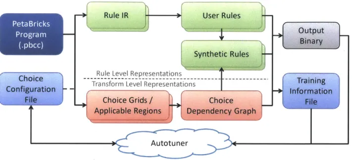
3.3 Autotuning System and Choice Framework . . . . 60
3.4 Runtime Library . . . . 62
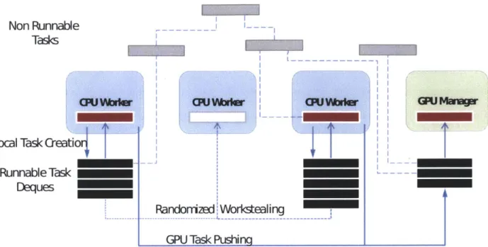
3.5 Code Generation for Heterogeneous Architectures . . . . 62
3.5.1 OpenCL Kernel Generation . . . . 63
3.5.2 Data Movement Analysis . . . . 64
. ... 69
3.5.5 GPU Choice Representation to the Autotuner . . . . 70
3.6 Choice Space Representation . . . . 72
3.6.1 Choice Configuration Files . . . . 72
3.7 Deadlocks and Race Conditions . . . . 73
3.8 Automated Consistency Checking . . . . 74
4 Benchmarks and Experimental Analysis 75 4.1 Fixed Accuracy Benchmarks . . . . 76
4.1.1 Symmetric Eigenproblem . . . . 76
4.1.2 Sort . . . 78
4.1.3 Matrix Multiply . . . . 80
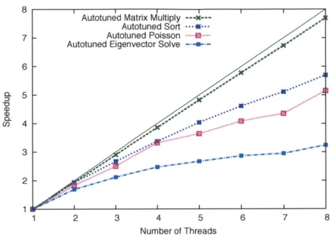
4.2 Autotuning Parallel Performance . . . . 80
4.3 Effect of Architecture on Autotuning . . . . 81
4.4 Variable Accuracy Benchmarks . . . . 82
4.4.1 Bin Packing . . . 83
4.4.2 Clustering . . . . 84
4.4.3 Image Compression . . . . 85
4.4.4 Preconditioned Iterative Solvers . . . . 86
4.5 Experimental Results . . . . 88
4.5.1 Analysis . . . . 88
4.5.2 Programmability . . . . 91
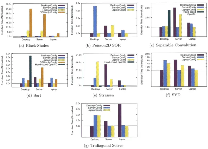
4.6 Heterogeneous Architectures Experimental Results . . . . 92
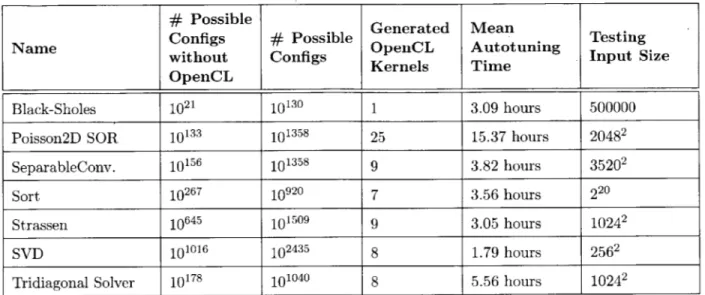
4.6.1 Methodology . . . . 92
4.6.2 Benchmark Results and Analysis . . . . 95
4.6.3 Heterogeneous Results Summary . . . 100
4.7 Summary . . . 102
5 Multigrid Benchmarks 103 5.1 Autotuning Multigrid . . . 104
5.1.1 Algorithmic choice in multigrid . . . 104
5.1.2 Full dynamic programming solution . . . 106
5.1.3 Discrete dynamic programming solution . . . 108
5.1.4 Extension to Autotuning Full Multigrid . . . 109
5.1.5 Limitations . . . 111
5.2 R esults . . . 112
5.2.1 Autotuned multigrid cycle shapes . . . 112
5.2.2 Performance . . . 116
5.2.3 Effect of Architecture on Autotuning . . . 124
6 The PetaBricks Autotuner 127 6.1 The Autotuning Problem . . . 128
6.1.1 Properties of the Autotuning Problem . . . 129
6.2 A Bottom Up EA for Autotuning . . . 130
6.3 Experimental Evaluation . . . 136
6.3.1 GPEA . . . 136 3.5.4 Memory Management
6.3.2 6.3.3 6.3.4 Experimental Setup . . . . INCREA vs GPEA ... Representative runs . . . . 7 Input Sensitivity 7.1 U sage . . . . 7.2 Input Aware Learning . . . . 7.2.1 A Simple Design and Its Issues . . . . 7.2.2 Design of the Two Level Learning . . . . 7.2.3 L evel 1 . . . . 7.2.4 Level 2 . . . . 7.2.5 Discussion of the Two Level Learning . . . . 7.3 Evaluation . . . . 7.3.1 Input Features and Inputs . . . . 7.3.2 Experimental Results . . . . 7.3.3 Input Generation . . . . 7.3.4 Model of Diminishing Returns with More Landmark 8 Online Autotuning
8.1 Competition Execution Model . . . . 8.1.1 Other Splitting Strategies . . . . 8.1.2 Time Multiplexing Races . . . . 8.2 SiblingRivalry Online Learner . . . . 8.2.1 High Level Function . . . . 8.2.2 Online Learner Objectives . . . . 8.2.3 Selecting the Safe and Seed Configuration . . . . 8.2.4 Adaptive Mutator Selection (AMS) . . . . 8.2.5 Population Pruning . . . . 8.3 Experimental Results and Discussion . . . . 8.3.1 Sources of Speedups . . . . 8.3.2 Load on a System . . . . 8.3.3 Migrating Between Microarchitectures . . . . 8.4 Hyperparameter Tuning . . . . 8.4.1 Tuning the Tuner . . . . 8.4.2 Evaluation metrics . . . . 8.4.3 R esults . . . . 8.4.4 Hyperparameter Robustness . . . .
Configurations
9 OpenTuner
9.1 The OpenTuner Framework . . . . 9.1.1 OpenTuner Usage . . . . 9.1.2 Search Techniques . . . . 9.1.3 Configuration Manipulator . . . 9.1.4 Objectives . . . . 9.1.5 Search Driver and Measurement 9.1.6 Results Database . . . . . 136 . 137 . 139 145 .148 . 148 148 149 150 152 156 157 158 159 162 164 167 169 169 170 171 172 173 174 174 176 177 177 178 180 182 183 185 187 189 193 194 195 197 198 201 201 202
. . . . 2 0 2 GCC/G++ Flags . . . .
H alide . . . . High Performance Linpack PetaBricks . . . . Stencil . . ... . . . . Unitary Matrices . . . . Results Summary . . . . 10 Related Work 10.1 Autotuning . . . . 10.2 Variable Accuracy . . . . 10.3 Multigrid . . . . 10.4 Autotuning Techniques. . 10.5 Online Autotuning . . . .
10.6 Autotuning Heterogeneous Architectures . 11 Conclusions Bibliography 215 . . . 2 1 5 . . . 2 1 9 . . . 2 2 1 . . . 2 2 1 . . . 2 2 2 223 227 251 9.2.1 9.2.2 9.2.3 9.2.4 9.2.5 9.2.6 9.2.7 . . . . 204 . . . . 206 207 . . . . 209 . . . . 211 . . . . 211 212 9.2 Experimental Results
Acknowledgments
This thesis includes text and experiments from a large subset of my publications while at MIT [8, 9. 11-13. 15-17, 37. 53. 110. 113]. The coauthors and collaborators of these publications deserve due credit and thanks: Clarice Aiello, Saman Amarasinghe, Cy Chan. Yufei Ding, Alan Edelman. Sam Fingeret, Sanath Jayasena., Shoaib Kamil. Kevin Kelley. Erika Lee, Deepak Narayanan, Marek Olszewski, Una-May O'Reilly, Maciej Pacula, Phitchaya Mangpo Phothilimthana. Jonathan Ragan-Kelley. Xipeng Shen. Michele Tartara., Kalyan Veeramachaneni, Yod Watanaprakornku, Yee Lok Wong, Kevin Wu, Minshu Zhan, and Qin Zhao.
I would specifically like to acknowledge some substantial contributions by: Cy Chan for multigrid benchmarks; Yufei Ding for input sensitivity; Maciej Pacula for bandit based online learning; Jonathan Ragan-Kelley for Halide (one of the six shown OpenTuner applications) and help on the GPU backend; and Phitchaya Mangpo Phothilimthana for the GPU backend and help providing feedback on this thesis.
Additionally, much of my academic work is beyond the scope of this thesis. but helped shape my experiences at MIT. This includes: collaboration on deterministic multi-threading [106, 107,109]. which was the primary project of Marek Olszewski. who is a dear friend, former office mate, and founder of Locu; self modifying code under software fault isolation [14], while I was a Google; and distributed checkpointing [10,43,44, 123] which was my focus as an undergraduate.
I am grateful for the advice and guidance of my advisor Saman Amarasinghe. I would also like to extend special thanks to my undergraduate advisor Gene Cooperman. Without their guidance I would not be where I am today. I would also like to thank the other members of the Commit group and those who provided feedback, both on draft manuscripts and on practice talks. I am
grateful to the members of my thesis committee, Armando Solar-Lezama and Martin Rinard for their feedback. I finally would like to thank my family and friends for their love and support.
This work is partially supported by NSF Award CCF-0832997, DOE Award DE-SC0005288,
DOD DARPA Award HR0011-10-9-0009, and an award from the Gigascale Systems Research Center. We wish to thank the UC Berkeley EECS department for generously letting us use one of their machines for benchmarking and NVIDIA for donating a graphics card used to conduct experiments. We would like, to thank Clarice Aiello for contributing the Unitary benchmark program. We gratefully acknowledge Connelly Barnes and Andrew Adams for helpful discussions and bug fixes related to autotuning the Halide project. This research used resources of the National Energy Research Scientific Computing Center, which is supported by the Office of Science of the U.S. Department of Energy under Contract No. DE-AC02-05CH11231.
Chapter 1
Introduction
The developers of languages and tools have invested a great deal of collective effort into extending the lifetime of software. To a large degree. this effort has succeeded. Millions of lines of code written decades ago are still being used in new programs. Early languages such as Fortran largely achieved their goals of having a single portable source code than can be compiled for almost any machines. Libraries and interfaces allow code to be reused in ways the original programmer could not foresee. Languages. such as Java. provide virtual machines allowing compiled bytecode to run on almost any system. We live in an era of write it once and use everywhere software.
What we have not yet achieved is performance portability. Hand coded optimizations for one system, often are not the best choice for another system. The result is obsolete optimizations that get carried to newer architectures in this portable software. A typical example of this can be found in the C++ Standard Template Library (STL) routine std: :stable-sort (Figure 1.1), distributed with the current version of GCC and whose implementation dates back to at least the 2001 SGI release of the STL. This legacy code contains a hard coded optimization, a cutoff constant of 15 between merge and insertion sort, that was designed for machines of the time. having 1/100th the memory of modern machines. Our tests have shown that higher cutoffs (around 60-150) perform much better on current architectures. However, because the optimal cutoff is dependent on architecture, cost of the comparison routine, element size. and parallelism, no single hard-coded
value will suffice. This type of hard coded optimization is typical in modern performance critical software.
/usr/include/c++/4.7.3/bits/stl-algo.h:
3508
///
Thisis
a helper function for the stable sorting routines. 3509 template<typename _RandomAccesslterator>3510 void
3511 __inplace -stable-sort
(_RandomAccesslterator
-_first3512 _RandomAccesslterator _-last
)
3513
{
3514 if
(--last
- __first < 15)3515
{
3516 std __insertion-sort
(
_first -_last)
3517 return;
3518
}
3519 -RandomAccesslterator __middle = __first +
(
_last - __first) /
2; 3520 std :_inplace-stable-sort(
_first , __middle );3521 std :_inplace-stable-sort (_middle ,_last )
3522 std :_merge-without _buffer ( _-first -_middle -_last
3523 __middle - __first
3524 _-last - __middle);
3525
}
Figure 1.1: Hard coded optimization constant 15 in std::stable-sort
While the paradigm of write once and run it everywhere is great for productivity, a major sacrifice made in these efforts is performance. Write once use everywhere often becomes write once slow everywhere. We need programs with performance portability, where programs can re-optimize themselves to achieve the best performance on widely different execution targets. The process of optimizing computer programs can be viewed as a search problem over the space of ways to implement a program. This search is traditionally manually conducted by the programmer, through iterative development and testing, and takes place in many domains. In high performance computing, there is constant optimization to fit algorithms to each new generation of supercomputers. The optimizations for one generation often will not be suitable for the next and may need to be undone. In areas such as graphics., optimizations must often be done to fit each hardware target a system may run on, which may range from a laptop to a powerful desktop computer with a large graphics card. In many web services applications, such as search, programs
will be optimized for quality of service so that they achieve the optimal results in a fixed time budget or a given level of service in the minimum time. In each of these domains., much of the difficulty of programming is in conducting a manual search over the solution space.
One of the most promising techniques to achieve performance portability is program autotuning. Rather than hard-coding optimizations, that only work for a single microarchitecture, or using fragile heuristics, program autotuning exposes a search space of program optimizations that can be explored automatically. Autotuning is used to search this optimization space to find the best configuration to use for each platform. Often these optimization search spaces contain complex decisions such as constructing recursive poly-algorithms to solve a problem. Autotuning can also be used to meet quality of service requirements of a program, such as sacrificing accuracy to meet hard execution time limits.
While using autotuners, instead of heuristics or models, for choosing traditional compiler optimizations can be successful at optimizing a single algorithm, when an algorithmic change is required to boost performance, the burden is put on the programmer to incorporate the new algorithm. If a composition of multiple algorithms is needed for the best performance, the programmer must write all the algorithms, the glue code to connect them together, and figure out the best switch over points. Making such changes automatically to the program requires heroic analysis or the analyses required is beyond the capability of all modern compilers. However, this information is clearly known to the programmer. The needs of modern computing require an either... or statement, which would allow the programmer to give a menu of algorithmic choices to the compiler. We also show how choices between different erogenous processing units, such as GPUs, can be automated by the PetaBricks compiler.
The need for a concise way to represent these algorithmic choices motivated the design of the PetaBricks programming language, which will be covered in detail in Chapter 2. Programs written in PetaBricks can naturally describe multiple algorithms for solving a problem and how they can be fit together. This information is used by the PetaBricks compiler and runtime, described in Chapter 3, to create and autotune an optimized hybrid algorithm. The PetaBricks system also optimizes and autotunes parameters relating to data distribution, parallelization, iteration, and
accuracy. The knowledge of algorithmic choice allows the PetaBricks compiler to automatically parallelize programs using the algorithms with the most parallelism when it is beneficial to do so.
Another issue that PetaBricks addresses is variable accuracy algorithms. Traditionally, language designers and compiler writers have operated under the assumption that programs require a fixed, precisely defined behavior; however, this is not always the case in practice. For many classes of applications, such as NP-hard problems or problems with tight computation or timing constraints, programmers are often willing to sacrifice some level of accuracy for faster performance. We broadly define these types of programs as variable accuracy algorithms. Often, these accuracy choices are hard coded into the program. The programmer will hand code parameters which provide good accuracy performance on some testing inputs. This choice over accuracy of the implementation can be viewed as another dimension in the solution space. An interesting example of variable accuracy can be found in Chapter 5, which shows our multigrid benchmarks. We show a novel dynamic programming approach for synthesizing multigrid V-cycles shapes tailored to a specific problem an accuracy target.
A large part of this thesis (Chapters 6 and 9) address the challenges developing techniques for autotuning. A number of novel techniques have been developed to efficiently search the search spaces created. The PetaBricks autotuner is based on an evolutionary algorithm (EA), however an off-the-shelf EA does not typically take advantage of shortcuts based on problem properties and this can sometimes make it impractical because it takes too long to run. A general shortcut is to solve a small instance of the problem first then reuse the solution in a compositional manner to solve the large instance which is of interest. Usually solving a small instance is both simpler (because the search space is smaller) and less expensive (because the evaluation cost is lower). Reusing a sub-solution or using it as a starting point makes finding a solution to a larger instance quicker. This shortcut is particularly advantageous if solution evaluation cost grows with instance size. It becomes more advantageous if the evaluation result is noisy or highly variable which requires additional evaluation sampling.
Another fundamental problem, which will be addressed in Chapter 7. is input sensitivity. For a large class of problems, the best optimization to use depends on the input data being processed.
For example. sorting an almost-sorted list can be done most efficiently with a different algorithm than one optimized for sorting random data. This problem is worse in autotuning systems, because there is a danger that the auotuner will create an algorithm specifically optimized for the inputs it is provided during tuning. This may be suboptimal for inputs later encountered in production or be a compromise solution that is not best for any one input but performs well overall. For many problems, no single optimized program exists which can match the performance of a collection of optimized programs autotuned for different subsets of the input space. This problem of input sensitivity is exacerbated by several features common to many classes of problems and types of autotuning systems. Many autotuning systems must handle large search spaces and variable accuracy algorithms with multiple objectives. They encounter inputs with non-superficial features that require domain specific knowledge to extract, Each of these challenges makes the problem of input sensitivity more difficult in a unique way.
Chapter 7 will present a general means of automatically determining what algorithmic optimization to use when different ones suit different inputs. While input sensitivity seems to be intertwined with the complexity of large optimization spaces and input spaces, we show that it can be resolved via simple extensions to our existing autotuning system. We show that the complexity of input sensitivity can be managed, and that a small number of input optimized programs is often sufficient to get most of the benefits of input adaptation.
In Chapter 8, we take a novel approach to online learning that enables the application of evolutionary tuning techniques to online autotuning. Our technique, called SiblingRivalry, divides the available processor resources in half and runs the current best algorithm on one half and a variation on the other half. If the current best finishes first, the variation is killed. the failure of the variation is reported to the online learning algorithm which controls the selection of both configurations for such "competitions" and the application continues to the next stage. If the variation finishes first, we have found a better solution than the current best. Thus, the current best is killed and the results from the variation are used as the program continues to the next stage. Using this technique, SiblingRivalry produces predictable and stable executions, while still exploiting an evolutionary tuning approach. The online learning algorithm is capable of adapting
to changes in the environment and progressively identifies better configurations over time without resorting to experiments that might deliver extremely slow performance. As we will show, despite the loss of resources, this technique can produce speedups over fixed configurations when the dynamic execution environment changes. To the best of our knowledge, SiblingRivalry is the first attempt at employing evolutionary tuning techniques to online autotuning computer programs.
Chapter 9 will present OpenTuner, a new framework for building domain-specific program autotuners. OpenTuner features an extensible configuration and technique representation able to support complex and user-defined data types and custom search heuristics. It contains a library of predefined data types and search techniques to make it easy to setup a new project. Thus, OpenTuner solves the custom configuration problem by providing not only a library of data types that will be sufficient for most projects, but also extensible data types that can be used to support more complex domain specific representations when needed.
1.1
Contributions
The overriding goal of this thesis work is to automate this optimization search and take it out of the hands over the programmer. The programmer should concisely define the search space, and then the compiler should perform the search. When the processors, coprocessors, accuracy requirements, or inputs programs should change themselves and adapt to work optimally in different each different environment. This provides performance portability, extends the life of software, and saves programmer effort.
To achieve this, this thesis has three main focuses:
* Designing language level solutions for concisely representing the implementation choice spaces of programs in ways that can be searched automatically.
" Developing process and compilation techniques to manage and explore these program search spaces.
" Creating novel autotuning techniques and search spaces representations to efficiently solve these search problems where prior techniques would fail or be inefficient.
The remainder of this subsection will expand on the contributions in each of these areas.
1.1.1 Language
The language level contributions in this work are realized in design and implementation of the PetaBricks programming language compiler.
" We introduce the PetaBricks programming language, which, to best of our knowledge, is the first language that enables programmers to express algorithmic choice at the language level.
" PetaBricks introduces the concept of the either ... or ... statement as a means to express recursive poly-algorithm choices.
" PetaBricks uses a declarative outer syntax to express iteration order choices around its imperative inner syntax. Multiple declarations in this declarative outer syntax allow the programmer to cleanly express algorithmic choices in handling boundary cases and iteration order dependency choices in a way that can automatically be searched by an autotuner.
" We have introduced the first language level support for variable accuracy. This includes support for multiple accuracy metrics and accuracy targets, which provide a general-purpose way for users to define arbitrary accuracy requirements in any domain and expands the scope of algorithmic choices that can be represented.
" PetaBricks introduces the concept of the for-enough loop, a loop whose input-dependent iteration bounds are determined by the autotuner.
" We introduce language level support for declaring variable accuracy input features, to enable programs that dynamically adapt to each input.
1.1.2 Process and Compilation
* While autotuners have exploited coarse-grained algorithmic choice at a programmatic level, to best of our knowledge PetaBricks is the first compiler that incorporates fine-grained
algorithmic choices in program optimization. PetaBricks includes novel compilation structures to organize and manage this choice space.
" We introduce a new model for online autotuning, called SiblingRivalry, where the processor resources are divided and two candidate configurations compete against each other in parallel. This solves the problem of exploring a volatile configuration space., by dedicating half the resources to a known safe configuration.
" We developed the first system to simultaneously address the interdependent problems of variable accuracy algorithms and input sensitivity.
* We introduce the first system which automatically determines the best mapping of programs in a high level language across a heterogeneous CPU/GPU mix of parallel processing units. including placement of computation. choice of algorithm, and optimization for specialized memory hierarchies. With this. a high-level, architecture independent language can obtain comparable performance to architecture specific. hand-coded programs.
1.1.3 Autotuning Techniques
The autotuning technique contributions of this work can be divided into two main areas. First. a number of novel techniques have been developed in the context of PetaBricks. The remaining contributions in the area of autotuning techniques are in the OpenTuner project., a new open source framework for building domain-specific multi-objective program autotuners.
" We have created a multi-objective, practical evolutionary autotuning algorithm for high-dimensional, multi-modal. and experimentally shown its efficacy on non-linear configuration search spaces up to 103000 possible configurations in size.
* We introduce a bottom-up learning algorithm that drastically improves convergence time for many benchmarks. It does this by using tests conducted on much smaller program instances to bootstrap the learning process.
" We show a novel dynamic programming solution to efficiently build tuned multigrid V-cycle algorithms that combine methods with varying levels of accuracy while providing that a final target accuracy is met. These autotuned V-cycle shapes are non-obvious and perform better than the cycle shapes used in practice.
" We have developed a technique for mapping variable accuracy code so that it can be efficiently autotuned without the search space growing prohibitively large. This is done by simultaneously autotuning for many different accuracy targets.
" We present a multi-armed bandit based algorithm for online autotuning. which, to the best of our knowledge, is the first application of evolutionary algorithms to the problem of online autotuning of computer programs.
" We show a through principled search of the parameter space of our multi-armed bandit algorithm that a single "robust" parameter setting exists. which performs well across a large suite of benchmarks.
" To solve the problem of input sensitive programs, we present a novel two level approach, which first clusters the input feature space into input classes and then builds adaptive overhead-aware classifiers to select between different input optimized algorithms for these classes, solves the problem of input sensitivity for much larger algorithmic search spaces than would be tractable using prior techniques.
" We offer a principled understanding of the influence of program inputs on algorithmic autotuning., and the relations among the spaces of inputs, algorithmic configurations. performance, and accuracy. We identify a key disparity between input properties. configuration. and execution behavior which makes it impractical to produce a direct mapping from input properties to configurations and motivates our two level approach.
" We show both empirically and theoretically that for many types of search spaces there are rapidly diminishing returns to adding more and more input adaption to a program. A little bit of input adaptation goes a long way, while a large amount is often unnecessary.
" We present OpenTuner, which is a general autotuning framework to describe complex search spaces which contain parameters such as schedules and permutations.
" OpenTuner introduces the concept of ensembles of search techniques to program autotuning, which allow many search techniques to work together to find an optimal solution.
" OpenTuner provides more sophisticated search techniques than typical program auotuners. This enables expanded uses of program autotuning to solve more complex search problems and pushes the state of the art forward in program autotuning in a way that can easily be adopted by other projects.
Chapter 2
The PetaBricks Language
This chapter will provide an overview of the base PetaBricks language and all extensions made to it over the course of this thesis work. The key features of the language, such as algorithmic choice and variable accuracy, will be introduced with example programs.
2.1
Sorting as an Example of Algorithmic Choice
As a motivation example, consider the problem of sorting. There are a huge number of ways to sort a list [31]. For example: insertion sort. quick sort, merge sort, bubble sort, heap sort. radix sort, and bucket sort. Most of these sorting algorithms are recursive, thus, one can switch between algorithms at any recursive level. This leads to an exponential number of possible algorithmic compositions that make use of more than one primitive sorting algorithm.
Since sorting is a well known problem, most readers will have some intuition about the optimal algorithm: for very small inputs, insertion sort is faster; for medium sized inputs, quick sort is faster (in the average case); and for very large inputs radix sort becomes fastest. Thus. the optimal algorithm might be a composition of the three, using quick sort and radix sort to recursively decompose the problem until the subproblem is small enough for insertion sort to take over. Once parallelism is introduced, the optimal algorithm gets more complicated. It often makes sense to use merge sort at large sizes because it contains more parallelism than quick sort (the merging performed at each recursive level can also be parallelized). Another aspect that impacts performance beyond
available parallelism is the locality of different memory access patterns of each algorithm, which can impact the cache utilization.
Even with this detailed intuition (which one may not have for other algorithms), the problem of writing an optimized sorting algorithm is nontrivial. Using popular languages today, the programmer would still need to find the right cutoffs between algorithms. This has to be done through manually tuning or using existing autotuning techniques that would require additional code to integrate (as discussed in Chapter 1). If the programmer puts too much control flow in the inner loop for choosing between a wide set of choices, the cost of control flow may become prohibitive. The original simple code for sorting will be completely obscured by this glue, thus making the code hard to comprehend., extend, debug, port and maintain.
PetaBricks solves this problem by automating both algorithm selection and autotuning in the compiler. The programmer specifies the different sorting algorithms in PetaBricks and how they fit together. but does not specify when each one should be used. The compiler and autotuner will experimentally determine the best composition of algorithms to use and the respective cutoffs between algorithms. This has added benefits in portability. On a different architecture, the optimal cutoffs and algorithms may change. The PetaBricks program can adapt to this by merely retuning.
Figure 2.1 shows a partial implementation of Sort in PetaBricks. The Sort function is defined taking an input array named in and an output array named out. The either... or primitive implies a space of possible polyalgorithms. The semantics are that when the ether... or statement is executed, exactly one of the clauses will be executed, and the choice of which sub block to execute is left up to the autotuner. In our example., many of the sorting routines (QuickSort, MergeSort, and RadixSort) will recursively call Sort again, thus, the either... or statement will be executed many times dynamically when sorting a single list. The autotuner uses evolutionary search to construct polyalgorithms which make one decision at some calls to the either... or statement, then different decisions in the recursive calls.
These polyalgorithms are realized through selectors (sometimes called decision trees) which efficiently select which algorithm to use at each recursive invocation of the either... or statement.
function Sort to out [n] from in [n]
{
either{
InsertionSort (out}
or{
1 2 3 4 5 6 7 8 9 10 11 12 13 14 15 16 in); in); in); in); , in);Figure 2.1: PetaBricks code for Sort
(a) Optimized for an Intel Xeon X5460 (b) Optimized for a Sun UltraSPARC T1 Figure 2.2: Example synthesized selectors for Sort.
QuickSort (out,
}
or
{
MergeSort (out,}
or
{
RadixSort (out,}
or{
BitonicSort (out}
}
Nc ON N f 1461Figure 2.2 shows two examples of selectors that might be synthesized by the autotuner for some specific input and architecture.
2.2
Iteration Order Choices
Current language constructs are too prescriptive in specifying an exact iteration order for loop nests. In order to take advantage of architectural features such as vectorization and cache hierarchies, compilers are forced to perform heroic analysis to find better iteration orders. This not only hinders the compilers ability to get the best performance but also requires the programmer to specify additional constraints beyond what is required to describe many algorithms. Natural mathematical notations such as sets and tensors do not provide an iteration order.
To expose iteration order choices to the compiler, PetaBricks does not require an outer sequential control flow, it uses a declarative outer syntax combined with an imperative inner syntax. The outer syntax defines parameterized data dependencies, which bring data into the local scope of each imperative block. The compiler must find a legal execution order that computes inputs before outputs and every output exactly once. The outer syntax can define multiple ways of computing the same value as another way of expressing algorithmic choice. This is done by defining multiple rules to compute the same region of data.
The language is built around two major constructs, transforms and rules. The transform, analogous to a function, defines an algorithm that can be called from other transforms, code written in other languages. or invoked from the command line. The header for a transform defines to and from arguments, which represent inputs and outputs, and through intermediate data used within the transform. The size in each dimension of these arguments is expressed symbolically in terms of free variables, the values of which must be determined by the PetaBricks compiler.
The user encodes choice by defining multiple rules in each transform. Each rule defines how to compute a region of data in order to make progress towards a final goal state. Rules have explicit dependencies parametrized by free variables set by the compiler. Rules can have different granularities and intermediate state. The compiler is required to find a sequence of rule applications that will compute all outputs of the program. The explicit rule dependencies allow automatic
parallelization and automatic detection and handling of corner cases by the compiler. The rule header references to and from regions which are the inputs and outputs for the rule. The compiler may apply rules repeatedly, with different bindings to free variables, in order to compute larger data regions. Additionally, the header of a rule can specify a where clause to limit where a rule can be applied. The body of a rule consists of C++-like code to perform the actual work.
Instead of outer sequential control flow, Petabricks users specify which transform to apply, but not how to apply it. The decision of when and which rules to apply is left up the compiler and runtime system to determine. This has the dual advantages of both exposing algorithmic choices to the compiler and enabling automatic parallelization. It also gives the compiler a large degree of freedom to autotune iteration order and storage.
Figure 2.3 shows an example PetaBricks transform, that performs matrix multiplication. The transform header is on lines 1 to 5, which defines the inputs outputs and 7 intermediate matrices which may or may not be used. The first rule (line 8 to 10) is the straightforward way of computing a single matrix element. With the first rule alone the transform would be correct, the remaining rules add choices. Rule 2 (lines 14 to 16) operated on a different granularity., a 4x4 tile, and could contain a vectorized version. Next come rules to compute the intermediate Mi though M7 defined in Strassen's algorithm. This intermediate data will only be used in the final 4 rules are chosen, which compute the quadrents of the output from MI to M7.
The PetaBricks transform is a side effect free function call as in any common procedural language. The major difference with PetaBricks is that we allow the programmer to specify multiple rules to convert the inputs to the outputs for each transform. Each rule converts parts or all of the inputs to parts or all of the outputs and may be implemented using multiple different algorithms. It is up to the PetaBricks compiler to determine which rules are necessary to compute the whole output, and the autotuner to decide which of these rules are most computationally efficient for a given architecture and input.
Taken together. the set of possible pathways through the graph of rules in a transform may be thought of as forming a directed acyclic dependency graph with various paths leading from the transform's inputs (represented as the graph's source) to the transform's outputs (represented as
transform StrassenMatrixMultiply from A[n, n] , B[n, n] to AB[n, n] using Ml[n/2, n/2] , M2[n/2, n/2] , M3[n/2, n/2] , M4[n/2, n/2], M5[n/2, n/2], M6[n/2, n/2], M7[n/2, n/2] {
/7
Base case 1: Compute a single element to(AB. cell (x, y) out)from(A.row(y) a, B.column(x) b) {
out = dot(a,b); I
// Base case 2: Vectorized version t to(AB.region(x, y, x + 4, y + 4) out from(A.region(0, y, n, y + 4) a,
B.region(x, 0, x + 4, n) b){
77
Compute intermediate data to(M m) from(A.region(0, 0, n/2, n/2) all, A.region(n/2, n/2, n, n) a22, B.region(0, 0, n/2, n/2) b1l, B.region(n/2, n/2, n, n) b22) using(tl[n / 2, n / 2], t2 [n/2, n/
spawn MatrixAdd(tl, all, a22);
spawn MatrixAdd(t2, b1, b22); sync;
StrassenMatrixMultiply (ml, tl , t2 I
o compute 16 elements at a time
.}
2])
{
// ... M2 through M7 rules omitted ...
//
Recursive case : Compute the4
quadrants using M1 through M7 to(AB.region(0, 0, n/2, n/2) c1l) from(Ml ml, M4 m4, M5 m5, M7 m7){ MatrixAddAddSub(cll , ml, m4, m7, m5); I to(AB.region(n/2, 0, n, n/2) c12) from(M3 m3, M5 m5){ MatrixAdd(c12, m3, m5); I to(AB.region(0, n/2, n/2, n) c21) from(M2 m2, M4 m4){ MatrixAdd(c21, m2, m4); I to(AB.region(n/2, n/2, n, n) c22) from(Ml ml, M2 MatrixAddAddSub(c22, m, m3, m6, m2);}
m2, M3 m3, M6 m6){Figure 2.3: PetaBricks code for MatrixMultiply I
the graph's sink). Intermediate nodes in the graph represent intermediate data structures produced and used during the computation of the output. The user specifies how to get to nodes from other nodes by defining rules. The rules correspond to the edges (or sometimes hyperedges) of the graph. which encode both the data dependencies of the algorithm, as well as the code needed to produce the edge's destinations from the sources.
In addition to choices between different algorithms, many algorithms have configurable parameters that change their behavior. A common example of this is the branching factor in recursively algorithms such as merge sort or radix sort. To support this PetaBricks has a tunable keyword that allows the user to export custom parameters to the autotuner. PetaBricks analyzes where these tunable values are used, and autotunes them at an appropriate time in the learning process.
PetaBricks contains many additional language features such as: %{ ...
}%
escapes used to embed raw C++ in the output file; a generator keyword for specifing a transform to be used to supply input data during training; matrix versions, with a A<O. .n> syntax, useful when definingiterative algorithms; rule priorities and where clauses are used to handle corner cases gracefully; and template transforms, similar to templates in C++. where each template instance is autotuned separately.
2.3
Variable Accuracy
Another issue that PetaBricks addresses is variable accuracy algorithms. This choice over accuracy of the implementation can be viewed as another dimension in the solution space. There are many different classes of variable accuracy algorithms.
One class of variable accuracy algorithms are approximation algorithms in the area of soft computing [165]. Approximation algorithms are used to find approximate solutions to computationally difficult tasks with results that have provable quality. For many computationally hard problems. it is possible to find such approximate solutions asymptotically faster than it is to find an optimal solution. A good example of this is BINPACKING. Solving the BINPACKING problem is NP-hard, yet arbitrarily accurate solutions may be found in polynomial time [50]. Like
many soft computing problems, BINPACKING has many different approximation algorithms, and the best choice often depends on the level of accuracy desired.
Another class of variable accuracy algorithms are iterative algorithms used extensively in the field of applied mathematics. These algorithms iteratively compute approximate values that converge toward an optimal solution. Often, the rate of convergence slows dramatically as one approaches the solution, and in some cases a perfect solution cannot be obtained without an infinite number of iterations [163]. Because of this, many programmers create convergence criteria to decide when to stop iterating. However, deciding on a convergence criteria can be difficult when writing modular software because the appropriate criteria may not be known to the programmer ahead of time.
A third class of variable accuracy algorithms are algorithms in the signal processing domain. In this domain, the accuracy of an algorithm can be directly determined from the problem specification. For example, when designing digital signal processing (DSP) filters, the type and order of the filter can be determined directly from the desired sizes of the stop., transition and pass-bands as well as the required filtering tolerance bounds in the stop and pass-bands. When these specifications change. the optimal filter type may also change. Since many options exist, determining the best approach is often difficult, especially if the exact requirements of the system are not known ahead of time.
To help illustrate variable accuracy algorithms in PetaBricks, we will first introduce a new example program. kmeans, which will used as a running example in this Section.
2.3.1 K-Means Example
Figure 2.4 presents an example PetaBricks program. kmeans. This program groups the input Points into a number of clusters and writes each points cluster to the output Assignments. Internally the program uses the intermediate data Centroids to keep track of the current center of each cluster. The rules contained in the body of the transform define the various pathways to construct the
Assignments data from the initial Points data. The transform can be depicted using the dependence graph shown in Figure 2.5, which indicates the dependencies of each of the three rules.
transform kmeans
from Points [n.,2]
/
Array7/
stores using Centroids[sqrt(n)
2] to Assignments[n]
{
Rule 1:
/
One possible initial set of pointsto(Centroids .column(i) c c=p.column(rand (0, n))
}
of points (each column x and y coordinates)
condition: Random
) from(Points p)
/
Rule 2:/
Another initial condition: Centerplus/
centers (kmeans++)to(Centroids c) from(Points p)
{
CenterPlus (c . p)
}
/
Rule 3:The kmeans iterative algorithm to(Assignments a) from(Points p.
while (true)
{
int change;AssignC lusters (a, change , p. if (change==0) return;
//
ReaNewClusterLocations(c, p, a);
}
}
Centroids c) c, a); ched fixed p{
ointFigure 2.4: PetaBricks code for kmeans.
{
initial
Rule 1 (run n times) Points Centroids Rule 2rns (run once) ule -+ Assignments
Input Intermediate Output
Figure 2.5: Dependency graph for kmeans example. The rules are the vertices while each edge represents the dependencies of each rule. Each edge color corresponds to each named data dependence in the pseudocode.
The first two rules specify two different ways to initialize the Centroids data needed by the iterative kmeans solver in the third rule. Both of these rules require the Points input data. The third rule specifies how to produce the output Assignments using both the input Points and intermediate Centroids. Note that since the third rule depends on the output of either the first or second rule, the third rule will not be executed until the intermediate data structure Centroids has been computed by one of the first two rules.
To summarize, when our transform is executed, the cluster centroids are initialized either by the first rule, which performs random initialization on a per-column basis with synthesized outer control flow, or the second rule, which calls the CenterPlus algorithm. Once Centroids is generated, the iterative step in the third rule is called.
2.3.2 Language Support for Variable Accuracy
To realize support for variable accuracy we extend the idea of algorithmic choice to include choices between different accuracies. We provide a mechanism to allow the user to specify how accuracy should be measured. Our accuracy-aware autotuner then searches to optimize for both time and accuracy. The result is code that probabilistically meets users' accuracy needs. Optionally, users can request hard guarantees (described below) that utilize runtime checking of accuracy.
transform kmeans
accuracy-inetric kIiwansaici(racy'N accu racy-variable k
from Points[n,2]
/7
Array of points (each column7/
stores x and y coordinates) using Centroids [k,2]to Assignments [n]
{
7/
Rule 1:/7
One possible initial condition: Random7/
set of pointsto(Centroids.column(i) c) from(Points p)
{
c=p. column(rand (0,n))}
7/
Rule 2:7/
Another initial condition: Centerplus initial7/
centers (kmeans++)to(Centroids c) from(Points p)
{
CenterPlus (c , p);
}
/7
Rule 3:7/
The kmeans iterative algorithmto(Assignments a) from(Points p, Centroids for-enough
{
int change;
AssignClusters(a, change, p, c, a);
if (change==0) return;
//
Reached fixe NewClusterLocations (c, p., a);}
dc)
{
point}
}
transform k.leasa((uracyfrom Assignmiiients i. Points
[n
2 to AccuracyAccuracy from( Assignimenits a. Poinits p){
return sqrt (2C/SumClusterDistaiiceSquared (a. p
)
}
Figure 2.6: PetaBricks code for variable accuracy kmeans. highlighted in light blue.)
Figure 2.6 presents our kmeans example with our new variable accuracy extensions. The updates to the code are highlighted in light blue. The example uses three of our new variable accuracy
features.
First the accuracy-metric, on line 2, defines an additional transform, kmeansaccuracy, which computes the accuracy of a given input/output pair to kmeans. PetaBricks uses this transform during autotuning and sometimes at runtime to test the accuracy of a given configuration of the kmeans transform. The accuracy metric transform computes the
>j2,
where Di is the Euclidean distance between the i-th data point and its cluster center. This metric penalizes clusters that are sparse and is therefore useful for determining the quality of the computed clusters. Accuracy metric transforms such as this one might typically be written anyway for correctness or quality testing, even when programming without variable accuracy in mind.The accuracy-variable k, on line 3 controls the number of clusters the algorithm generates by changing the size of the array Centroids. The variable k can take different values for different input sizes and different accuracy levels. The compiler will automatically find an assignment of this variable during training that meets each required accuracy level.
The for-enough loop on line 26 is a loop where the compiler can pick the number of iterations needed for each accuracy level and input size. During training the compiler will explore different assignments of k., algorithmic choices of how to initialize the Centroids. and iteration counts for the for-enough loop to try to find optimal algorithms for each required accuracy.
2.3.3 Variable Accuracy Language Features
PetaBricks contains the following language features used to support variable accuracy algorithms:
* The accuracy-metric keyword in the transform header allows the programmer to specify the name of another user-defined transform to compute accuracy from an input/output pair. This allows the compiler to test the accuracy of different candidate algorithms during training. It also allows the user to specify a domain specific accuracy metric of interest to them.
" The accuracy-variable keyword in the transform header allows the user to define one or more algorithm-specific parameters that influence the accuracy of the program. These variables are
set automatically during training and are assigned different values for different input sizes. The compiler explores different values of these variables to create candidate algorithms that meet accuracy requirements while minimizing execution time. An accuracy variable is the same as a tunable except that it provides some hints to the autotuner about its effect.
" The accuracy-bins keyword in the transform header allows the user to define the range of accuracies that should be trained for and special accuracy values of interest that should receive additional training. This field is optional and the compiler can add such values of interest automatically based on how a transform is used. If not specified, the default range of accuracies is 0 to 1.0.
" The for-enough statement defines a loop with a compiler-set number of iterations. This is useful for defining iterative algorithms. This is syntactic sugar for adding an accuracy-variable to specify the number of iterations of a traditional loop.
" The semantics for calling variable accuracy transforms is also extended. When a variable accuracy transform calls another variable accuracy transform (including recursively), the required sub-accuracy level is determined automatically by the compiler. This is handled by making each function polymorphic on accuracy.
When a variable accuracy transform is called from fixed accuracy code, the desired level of accuracy must be specified. We use template-like, "<N>", syntax for specifying desired accuracy. This syntax may also be optionally used in variable accuracy transforms to prevent the automatic expansion described above.
* The keyword verify-accuracy in the rule body directs the compiler to insert a runtime check for the level of accuracy attained. If this check fails the programmer can insert calls to retry with the next higher level of accuracy or the programmer can provide custom code to handle this case. This keyword can be used when strict accuracy guarantees, rather than probabilistic guarantees, are desired for all program inputs.
2.3.4
Accuracy Guarantees
PetaBricks supports the following three types of accuracy guarantees:
" Statistical guarantees are the most common technique used, and the default behavior of our system. They work by performing off-line testing of accuracy using a set of program inputs to determine statistical bounds on an accuracy metric to within a desired level of confidence. Confidence bounds are calculated by assuming accuracy is normally distributed and measuring the mean and standard deviation. This implicitly assumes that accuracy distributions are the same across training and production inputs.
" Runtime checking can provide a hard guarantee of accuracy by testing accuracy at runtime and performing additional work if accuracy requirements are not met. Runtime checking can be inserted using the verify-accuracy keyword. This technique is most useful when the accuracy of an algorithm can be tested with low cost and may be more desirable in case where statistical guarantees are not sufficient.
" Domain specific guarantees are available for many types of algorithms. In these cases, a programmer may have additional knowledge, such as a lower bound accuracy proof or a proof that the accuracy of an algorithm is independent of data., that can reduce or eliminate the cost of runtime checking without sacrificing strong guarantees on accuracy. In these cases the
accuracy-metric can just return a constant based on the program configuration.
As with variable accuracy code written without language support, deciding which of these techniques to use with what accuracy metrics is a decision left to the programmer.
2.4
Input Features
For a large class of problems, the best optimization to use depends on the input data being processed. We broadly call this feature of algorithms input sensitivity and will discuss our handling of them in detail in Chapter 7.
unction Sort o out [n] rom in [n] nput-feature Sortediiess 1 2 3 5 6 7 8 9 10 11 12 13 14 15 16 17 '9 20 21 22 23 24 26 27 28 29 30 31 32 33 34 36 37 38 39 40 41 42 43 44 D11plicat ion t , in); n); n ) ; n ); in) (o.o . 1 ()) int sortedcol1t= 0: init
count
=0;,iut Ste =) (n t ) (level *n)
for(int i=0: i+step<n; i+=step) { if( in
il]
<= iii[i+step])/ 7In.emi(t,
for
c0rr(ctly Ord(r(d sortedcount += 1: } counlt +=1
if(count > 0) so rt edn ess -else // (double) count ; s0rtedness
-0.0:
}function Ditplicat ion from in [i]
to (111plication
Figure 2.7: PetaBricks code for Sort with input features. (The new input feature code is highlighted
f
t
i]{
either{
InsertionSort (ou}
or{
QuickSort (out, i}
or
{
MergeSort (out, i}
or{
RadixSort (out i}
or
{
BitonicSort (out,}
}
function Sorte(dness fromi in [it]to
smrtedelicstunable double
leve
{
PetaBricks provides language support for input sensitivity by adding the keyword input-feature, shown on lines 4 and 5 of Figure 2.7. The input-feature keyword specifies a programmer-defined function, a feature extractor, that will measure some domain specific property of the input to the function. A feature extractor must have no side effects, take the same inputs as the function, and output a single scalar value. The autotuner will call this function as necessary.
Feature extractors may have tunable parameters which control their behavior. For example, the
level tunable on line 23 of Figure 2.7. is a value that controls the sampling rate of the sortedness feature extractor. Higher values will result in a faster, but less accurate measure of sortedness. Tunable is a general language keyword that specifies a variable to be set by the autotuner and two values indicating the allowable range of the tunable (in this example between 0.0 and 1.0).
2.5
A More Complex Example
To end the chapter we show a more complex example PetaBricks program, Convolution, and its performance characteristics when mapped to different GPU/CPU targets. We will show the power of algorithmic choice previewing the results for convolution. The full set of results an be found in Chapter 4.
Figure 2.8 shows the PetaBricks code for Separable Convolution. The top-level transform computes Out from In and Kernel by either computing a single-pass 2D convolution, or computing two separate ID convolutions and storing intermediate results in buffer. Our compiler maps this program to multiple different executables which perform different algorithms (separable vs. 2D blur), and map to the GPU in different ways. This program computes the convolution of a 2D matrix with a separable 2D kernel. The main transform (starting on line 1) maps from input matrix
In to output matrix Out by convolving the input with the given Kernel. It does this using one of two rules: