Publisher’s version / Version de l'éditeur:
Journal of chemistry theory and computation, 6, 5, pp. 1608-1621, 2010-01-01
READ THESE TERMS AND CONDITIONS CAREFULLY BEFORE USING THIS WEBSITE. https://nrc-publications.canada.ca/eng/copyright
Vous avez des questions? Nous pouvons vous aider. Pour communiquer directement avec un auteur, consultez la première page de la revue dans laquelle son article a été publié afin de trouver ses coordonnées. Si vous n’arrivez pas à les repérer, communiquez avec nous à PublicationsArchive-ArchivesPublications@nrc-cnrc.gc.ca.
Questions? Contact the NRC Publications Archive team at
PublicationsArchive-ArchivesPublications@nrc-cnrc.gc.ca. If you wish to email the authors directly, please see the first page of the publication for their contact information.
NRC Publications Archive
Archives des publications du CNRC
This publication could be one of several versions: author’s original, accepted manuscript or the publisher’s version. / La version de cette publication peut être l’une des suivantes : la version prépublication de l’auteur, la version acceptée du manuscrit ou la version de l’éditeur.
For the publisher’s version, please access the DOI link below./ Pour consulter la version de l’éditeur, utilisez le lien DOI ci-dessous.
https://doi.org/10.1021/ct9006025
Access and use of this website and the material on it are subject to the Terms and Conditions set forth at
Rapid Prediction of Solvation Free Energy. 1. An Extensive Test of
Linear Interaction Energy (LIE)
Sulea, Traian; Corbeil, Christopher R.; Purisima, Enrico O.
https://publications-cnrc.canada.ca/fra/droits
L’accès à ce site Web et l’utilisation de son contenu sont assujettis aux conditions présentées dans le site LISEZ CES CONDITIONS ATTENTIVEMENT AVANT D’UTILISER CE SITE WEB.
NRC Publications Record / Notice d'Archives des publications de CNRC:
https://nrc-publications.canada.ca/eng/view/object/?id=db942382-0c5f-45a5-93de-fc05ec724686 https://publications-cnrc.canada.ca/fra/voir/objet/?id=db942382-0c5f-45a5-93de-fc05ec724686Rapid Prediction of Solvation Free Energy. 1. An
Extensive Test of Linear Interaction Energy (LIE)
Traian Sulea, Christopher R. Corbeil, and Enrico O. Purisima*
Biotechnology Research Institute, National Research Council Canada, 6100 Royalmount AVenue, Montreal, Quebec H4P 2R2, Canada
Received November 17, 2009
Abstract:The present study provides a comprehensive systematic analysis on the applicability of the linear interaction energy (LIE) approximation to the prediction of gas-to-water transfer (hydration) free energy. The study is based on molecular dynamics simulations in explicit solvent for an extensive and diverse hydration data set comprising 564 neutral compounds with measured hydration free energies, including a “traditional” data set and the more challenging drug-like SAMPL1 data set. A highly correlative LIE model was achieved without empirical scaling of the solute-solvent interaction energy terms along with a cavity term calibrated to the experiment. This model was particularly accurate for the “traditional” data set and of acceptable accuracy for the SAMPL1 data set, with mean-unsigned-errors below 1 kcal/mol and slightly above 2 kcal/mol, respectively. We have analyzed the sensitivity of the LIE model to several parameters such as continuum correction terms applied outside the explicit water shell, the impact of various charging methods, the applicability of single-conformer representation of the solute, and the inclusion of internal energy terms. The parameters with the greatest sensitivity are the charging methods used, with AM1BCC-SP (without AM1 geometry optimization) charges favored over AM1BCC-OPT and RESP charges. The inclusion of the change in intramolecular van der Waals and electrostatic energies between the solution and gas phases can also lead to improved prediction accuracies. Functional group based error analysis identified several chemical classes as minor outliers with systematic errors. A direct comparison of the LIE and free energy perturbation (FEP) approaches using the same force field and charging method shows that the LIE approximation is at least as accurate as the FEP approach with a reduction of computing time by at least 1 order of magnitude.
Introduction
Hydration (aqueous solvation) of molecules plays an im-portant role in biological, chemical, and industrial processes, as exemplified by the change in hydration upon complex formation. This change in hydration is a critical component of binding affinities in aqueous solution;1-3hence, simulation methods that predict absolute binding free energies require accurate hydration models. Implementation of accurate hydration models in scoring functions would benefit
promis-ing applications such as virtual screenpromis-ing in drug discovery. Over the years, much effort has been expended in developing and parametrizing solvation models at various levels of theory.4-10 Accurate prediction of hydration free energies still remains a challenge for computational methods, as underscored by scientific community efforts like the SAM-PL1 blind prediction challenge organized recently by Open-Eye, Inc.11 In general, simulation methods fall into two groups depending on whether they treat the water implicitly or explicitly.
Implicit hydration models (also known as continuum models) have the benefit of speed, but they break down on describing effects that relate to the discrete nature of water * To whom correspondence should be addressed. Phone:
514-496-6343. Fax: 514-496-5143. E-mail: enrico.purisima@ cnrc-nrc.gc.ca.
10.1021/ct9006025 Published 2010 by the American Chemical Society
due to ordering in the first solvation shell around solutes, e.g., charge asymmetry or dependence of ion pairing on molecular shape.12,13 Such effects are captured by explicit solvation models, which are more transferable than the continuum models but are generally prohibitively slow for many routine applications. The current challenge for the computational chemistry community is to develop hydration models that are as physics-based as the explicit models but have the speed of continuum models, as both accuracy and speed are required for practical applications in drug discov-ery. One such example is restoring charge asymmetry observed with explicit models within continuum models, which has been recently reported.14 Even with these ad-vances, implicit models still require further calibration on either experimental hydration free energies or computed energies from explicit-solvent simulations.
The free energy of solvation can be calculated in explicit solvent from molecular dynamics (MD) simulations using path methods like free energy perturbation (FEP) and thermodynamic integration (TI),15which require slow trans-formations between the end points of the hydration process (the gas phase and water-solvated state). Typically, such methods require long simulation times to reach convergence. Applications of the FEP approach to the hydration of small molecules have been recently reported with good success.16-18 The linear interaction energy (LIE) is an attractive ap-proximation of the rigorous full FEP methodology, where only the average interaction energies are calculated at the end-points of the process. This approximation has a signifi-cant impact on shortening the required MD simulation time. The LIE approximation has been applied to the problem of protein-ligand binding in solution with adjustable parameters for the interaction terms.19-25Linear response theory, which is deeply rooted in fundamental Gibbs inequalities, can provide remarkably accurate descriptions of the process of filling aqueous cavities with nonpolar, polar, or charged molecules.26Hydration of a small set of organic molecules has been studied previously with LIE in explicit solvent using Monte Carlo simulations and a calibrated cost of cavity formation27 and was later shown not to require empirical scaling of the solute-solvent interaction terms.24 More recently, linear response theory has been also applied to a hydration data set consisting of 194 simple neutral and ionic compounds. These semiempirical LIE models of hydration consisted of functional class-dependent empirical scaling of solute-solvent electrostatic interaction energies from fitting to simulated FEP data, and empirical scaling of the nonpolar term from fitting directly to the experimental data for the entire hydration data set.28
While the application of the LIE approximation to the calculation of hydration free energy is not a new idea, the present study is based on molecular dynamics simulations in explicit solvent for a significantly larger and more diverse hydration data set than previously analyzed. The set is comprised of 564 neutral compounds with measured hydra-tion free energies, including 501 “tradihydra-tional” simpler compounds used by Mobley et al.,16,29 and the drug-like SAMPL1 data set.11The inclusion of the 63 highly diverse, densely polyfunctional, neutral polar compounds, which
encompass larger magnitudes of hydration free energies and molecular weights, make the newer SAMPL1 testing data set more challenging than previous testing data sets.11The SAMPL1 blind challenge operated by first releasing the molecules to the public followed by the release of experi-mental transfer free energies after a few months. A number of continuum and explicit-solvent methods were tested, most of them in the prospective mode,17,30-32while results with two other methods were included retrospectively.33,34
We have analyzed the sensitivity of the LIE model to several parameters that we believe are important for the accuracy of the model and for calibration of a continuum model based on these results. These include continuum corrections to infinity, charging method, solute flexibility, and internal energy terms. We have opted not to fit the scaling parameters for the solute-solvent interaction energy terms to FEP data as in a previous study28but rather maintain the idealized theoretical values for these scaling parameters (1 for dispersive and 0.5 for electrostatic solute-solvent interactions) derived from the linear response theory.24,26By assuming an idealized linear response, we simplify the model and avoid the danger of model overfitting, while maintaining the theoretical rigor of a physically sound if albeit idealized model. It is a surprisingly good approximation. It is also important to compare the results from the LIE approach directly with those from the more rigorous FEP calculations. That is, the speedup advantage of LIE over FEP is attractive only if the accuracy of the prediction is maintained. This is possible since both data sets have been very recently studied with the FEP method with the same force field and charges,16,17thus allowing a direct comparison between LIE and FEP data.
A major motivation for this work is to generate the individual components of hydration free energy, electrostatics and van der Waals energies, both of which are experimentally inaccessible. This data will then be used to train the respective components of purely continuum solvation models with the aim of having this model mimic an explicit solvent simulation (see accompanying paper35).
Materials and Methods
Hydration Data Sets. A data set consisting of experi-mental hydration free energies for 501 neutral organic small molecules were taken from the Supporting Information provided by Mobley et al.16We followed the same approach of Mobley et al.,16not to include molecular ions in the study data set due to uncertainties in experimental data. The data set was split into a training set of 200 compounds used only for calibrating the cost of cavity formation in water and a testing data set of 301 compounds. In the training set, we included mostly rigid representatives of the various chemical classes, with the majority of compounds being monofunc-tional, and only a few polyfunctional compounds were included to increase coverage of some functional groups. The testing data set mirrors the training data set in terms of chemical class representation for monofunctional compounds but differs from the training analogs by having increased flexibility and containing a larger collection of polyfunctional
compounds. The SAMPL1 data set11 consists of 63 drug-like, diverse, polyfunctional, neutral polar compounds and spans a wider range of transfer free energies and molecular weights in comparison to the training and testing data sets. Details on the composition of the training and testing and SAMPL1 data sets are provided in the Supporting Informa-tion (Table S1).
Hydration Models.The following implementation of the LIE approach19,20,24,26,27was used to describe electrostatic, van der Waals, and cavity contributions to solvation:
where all terms represent averages (〈...〉) over snapshots from MD simulations. Here, 〈ES-WCoul〉e12Å and 〈ES-WvdW1〉e12Å are the average Coulomb and van der Waals interaction energies of the solute with explicit water molecules within 12 Å, respectively. We applied the ideal theoretical values of 0.5 and 1 for the R and β scaling factors of electrostatic and van der Waals average interaction energy terms,26 respec-tively, in eq 1, shown to yield good predictions of experi-mental hydration free energies on a limited data set.24,27 Following previous work,27 the cavity contribution is ex-pressed as a linear dependence on the average molecular surface area of the solute, 〈MSA〉, with the cavity surface coefficient,γcav, and a constant, C. These parameters were determined from a linear fit using Microsoft Excel to pseudoexperimental cavity energies obtained by subtracting the electrostatic and van der Waals contributions from experimental hydration free energies for the training data set.
Continuum-model correction terms were added outside the 12 Å shell of explicit water in order to capture the bulk solvent contribution to infinity. The average implicit elec-trostatic solvation outside the explicit water shell, 〈GSRF〉12Å-∞, includes reaction field energy contributions from the interac-tions between (a) the solute charges and their induced surface-charge density, GS-(σS)12Å
RF
, (b) the solute charges and the induced surface charge density due to the explicit water-shell charges, GS-(σW)12Å
RF
, and (c) the explicit water-shell charges and the induced surface-charge density due to solute charges, GW-(σS)12Å
RF
(eq 2).
Operationally, this external electrostatic solvation term was calculated by subtracting the reaction field energy between the explicit water charges and their induced surface-charge density, GW-(σW)12Å
RF
(calculated by setting solute charges to zero) from the entire reaction field energy of the solute plus the explicit water shell, GSW-(σSW)12Å
RF
. All induced surface-charge densities were calculated at the molecular surface of the 12 Å shell of explicit water solvating the solute at each
particular MD snapshot, using the boundary element method (BEM) implemented in the BRI-BEM program.36,37 All molecular surface calculations were carried out with a variable-radius probe.38
The continuum solute-solvent van der Waals interaction outside the explicit water shell, averaged over the MD trajectory, 〈EScvdW〉12Å-∞, was calculated as described by Floris et al.39,40Briefly, the discrete surrounding water molecules are replaced by a continuum of uniform density distribution, and the solute-solvent van der Waals interaction is taken to be proportional to the integral of the solute-continuum interaction over all of space. For ease of computation, the volume integral is transformed into a surface integral typically at the solute-solvent boundary defined by the solvent-accessible surface. Here, the surface integral was evaluated at the solvent-accessible surface around the 12 Å shell of explicit water. For the dispersion (attractive) component of the 6-12 Lennard-Jones potential, that leads to
where rijis the vector from solute atom i to patch j of the
solvent-accessible surface around the 12 Å shell of explicit water, njis the surface normal at j, SAjis the area of j, and
FN is the solvent number density. The atomic dispersion parameters Biwwere taken from the TIP3P and GAFF force
field41without scaling.
We also extended the LIE approach to include the difference in the average intramolecular energy of the solute in the aqueous phase, Eaqintra, and in the gas phase, Egasintra:
where the intramolecular energies are comprised of molecular mechanics force field bond stretching, angle bending, torsional (including improper corrections), 1-4 and 1-5 van der Waals, and 1-4 and 1-5 Coulombic electrostatic energies. We also considered excluding the covalent terms (bond stretching, angle bending, and dihedral and improper torsions) from the intramolecular energy.
Explicit-Solvent Simulations and Solute Parameters.
Single-conformation molecular geometries for the training, testing, and SAMPL1 data sets were downloaded from the appropriate sources11,16and refined by energy minimization with the Merck Molecular Force Field (MMFF94)42 and a 4R distance-dependent dielectric constant, up to a gradient of 0.01 kcal mol-1Å-1, in SYBYL 8 (Tripos, Inc. St. Louis, MO). These geometries were then used to calculate partial atomic charges with different methods. Solute atomic partial charges were calculated with the AM1BCC method43,44 〈GSRF〉12Å-∞) 〈(GS-(σ S)12Å RF + GS-(σ W)12Å RF + GW-(σ S)12Å RF )〉 ) 〈(GSW-(σ SW)12Å RF - GW-(σ W)12Å RF )〉 (2) 〈EScvdW〉 ) -FN
∑
i solute atoms∑
j patches 1 3 Biw dij6rij· njSAj (3)implemented within QUACPAC (OpenEye, Inc., Santa Fe, NM), with AM1 geometry optimization (AM1BCC-OPT) or without AM1 geometry optimization (single-point calcula-tion, AM1BCC-SP), as well as with the two-stage RESP method.45,46RESP atomic partial charges were fitted to the electrostatic potential from in Vacuo single-point calculations at the 6-31G* level (3-21G level for iodine-containing compounds) using GAMESS.47
Molecular dynamics simulations were carried out using AMBER 9 software48with the general AMBER force field (GAFF) parameters41 assigned to the solutes with PARMCHK and ANTECHAMBER,49 and using the TIP3P water parameters50,51 for the solvent. Solute molecules were solvated in a truncated octahedron of water extending 12 Å away from the solute. Applying harmonic restraints with force constants of 10 kcal mol-1Å-2to all solute atoms, the system was energy-minimized first, followed by heating from 100 K to 300 K over 25 ps in the canonical ensemble (NVT), and by equilibrating to adjust the solvent density under 1 atm of pressure over 25 ps in the isothermal-isobaric ensemble (NPT) simula-tion. The harmonic restraints were then reduced to zero, and a 2 ns production NPT run was obtained with snapshots collected every 10 ps, using a 2 fs time-step and 9 Å nonbonded cutoff. The Particle Mesh Ewald (PME) method52was used to treat long-range electrostatic interactions, and bond lengths involving bonds to hydrogen atoms were constrained by SHAKE.53 Separate MD simulations were carried out for the different charging methods of the solute molecules. Also, separate MD simulations were carried out with unconstrained (flexible) or constrained (rigid) solute molecule during the 2 ns production phase. In the latter case, the harmonic potential of 10 kcal mol-1Å-2on the solute atoms was maintained during the course of the entire MD protocol. Similar MD protocols were applied to carry out gas-phase simulations for all molecules with full solute flexibility and for all charge models using a 2 fs time step. All averages were calculated for 100 snapshots at 10 ps intervals from the last nanosecond of the 2 ns trajectories.
Bootstrapped statistical analyses were carried out for 5000 samples using the boot library within the R software.54 In order to help identify systematic prediction errors, functional group assignment for the compounds in the testing subset was carried out with CHECKMOL.55Since CHECKMOL only identifies if a group is present, further manual groupings were created for molecules that only contain one type of a functional group (see Table S2, Supporting Information).
Results and Discussion
We explored hydration free energy calculations within the LIE formalism based on MD simulations in explicit solvent on three data sets with measured water-to-vacuum transfer free energies: the more traditional training and testing data sets16,29and the challenging drug-like SAMPL1 data set.11 We will start by calibrating an empirical term for the cost of cavity formation in water, which is not directly provided by the force-field energy terms in the LIE approach. The LIE results for the case of flexible solutes and the
AM1BCC-SP charge model will be described first vis-a`-vis experimental data. We will separately analyze the effects of (1) removing the bulk-solvent continuum correction to infinity, (2) chang-ing the solute chargchang-ing method, (3) uschang-ing a schang-ingle-conforma- single-conforma-tion representasingle-conforma-tion of the solute, and (4) incorporating the internal energy difference between the two media on the accuracy of LIE predictions of hydration free energies. Functional group analysis will then be carried out to single out systematic outliers and problematic groups and try to identify potential sources of errors. The LIE prediction accuracy and functional group analysis of errors will be compared with published FEP alchemical calculations that are more computationally demanding but are thought to be more accurate, or at least more rigorous. Values for LIE components and predicted hydration free energies for all molecules can found in Table S3 (Supporting Information).
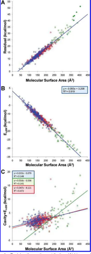
Deriving the Cavity Contribution.The dispersive (van der Waals) and electrostatic (Coulombic) solute-solvent interactions are well described by linear response theory, which implies Gaussian distributions of the energy fluctua-tions associated with these interacfluctua-tions.26On the other hand, the formation of a cavity the size of a molecule in water is not a linear process, which means that cavity formation fluctuations are significantly non-Gaussian. The cost of cavity formation in water, mainly of entropic nature, should in principle be directly related to the size of the cavity. Since in the LIE approach this term is not captured by the force-field-based interaction energy terms, we sought a linear relationship to the molecular surface area (MSA) of the solute in order to calibrate the cavity term. We started with the LIE model described in eq 1 and MD simulations with fully flexible solutes and AM1BCC-SP atomic charges. We defined a pseudoexperimental cavity contribution as the residual between the experimental hydration free energy and the calculated electrostatic and van der Waals solute-solvent interaction energies. Using the training set of 200 compounds, we obtained a robust linear correlation between the pseu-doexperimental cavity cost and the MSA (Figure 1A), with a bootstrapped squared correlation coefficient of 0.923 ( 0.015 and a slope and intercept (γ and C, respectively, in eq 1) of 0.108 ( 0.002 kcal mol-1Å-2and -3.298 ( 0.283 kcal/mol, respectively (Table 1).
The derived area coefficient, γ, is surprisingly close to the macroscopic surface tension of water, which is 0.105 kcal mol-1Å-2(converted from 72.75 dyn/cm at 20 °C).56 Other simulations have also yielded microscopic surface tensions of water close to the macroscopic one. Postma et al. used MD simulations with explicit water to investigate the dependence of free energy of cavity formation on the cavity size.57 The calculated free energies of formation of various sizes of spherical cavities were then related to the cavity radius using a quadratic polynomial. The coefficient of the squared term is then the calculated surface tension for cavities with radii not close to zero. They obtained a surface tension of 0.067 N/m or 0.096 kcal mol-1 Å-2. Prevost et al.58again using explicit water molecules and free energy perturbation methods gave a coefficient of 0.095 kcal mol-1 Å-2.
We used the two cavity parameters,γ and C, calibrated on the training data set, to predict the cavity contributions for testing data sets. The validity of this extrapolation can be judged from the relationship between pseudoexperimental cavity contribution and the MSA for the training, testing, and SAMPL1 data sets totalling 564 compounds (Figure 1A). The linear relationship calibrated on the training data set extends very well to the testing data set (γ ) 0.097 kcal mol-1 Å-2, C ) -1.869 kcal/mol) and also to most compounds of the SAMPL1 data set (γ ) 0.126 kcal mol-1 Å-2, C ) -7.118 kcal/mol), up to an MSA of about 350 Å2. For the larger compounds from the SAMPL1 data set, the calibrated cavity parameters appear to underestimate their pseudoexperimental (residual) cavity cost, which is also reflected by the larger slope (γ) value obtained by fitting directly to SAMPL1 data set (Table 1). Although this behavior may suggest the existence of nonlinear components in the dependence of the cavity term to the MSA, we also note that these larger compounds are sulfoneurea analogs and thus belong to the same functional class (filled circles in Figure 1). It is possible that the apparent steeper surface area dependence of the cavity term for these compounds is only compensating for other factors, e.g., limitations of the molecular mechanics force-fields to accurately describe the interaction energy terms for this functional group, as previ-ously suggested.17Indeed, most of the current state-of-the-art solvation methods when applied to the SAMPL1 data set failed miserably on these sulfoneurea analogs,17,31-33 although some of the QM-based methods seem to provide a better agreement to experiment for some of the sulfoneurea analogs.30,34
Total Nonpolar Component.The solute-solvent van der Waals interaction energy also correlates well with the MSA (Figure 1B). However, the total nonpolar contribution to solvation, comprising the cavity cost and the solute-solvent van der Waals interaction energy, does not correlate with the solute surface area (Figure 1C), due to the strong anticorrelation between these terms. This lack of correlation is particularly pronounced for compounds from the training and testing data sets, which mirrors the results reported for these types of compounds based on FEP simulations in explicit water.16,18Our analysis of the drug-like SAMPL1 compounds, which have larger surface areas, shows only a moderate correlation (Figure 1C) between the total nonpolar solvation and the MSA for this data set (R2of 0.472). Clearly, a single linear surface-area-dependent term cannot describe the total nonpolar component of solvation.
Figure 1. Deriving the cavity contribution. (A) Linear
relation-ship between pseudoexperimental (residual) cavity contribution and the MSA for the training (blue symbols) and testing (red symbols) data sets and for the SAMPL1 (green symbols) data set. The plotted data correspond to MD simulations with flexible solute and AM1BCC-SP charges. Only the regression line for the training data set is shown, since this is used to predict the cavity contribution for the testing and SAMPL1 data sets. Filled circle points correspond to 5 sulfoneurea analogs from the SAMPL1 data set. (B) Correlation between the solute-solvent van der Waals interaction energy and the molecular surface area of the solute for the same LIE model. (C) Scatter plot of the total nonpolar term to solvation and the molecular surface area of the solute for the same LIE model. Regression lines are shown for each data set and are colored as the corresponding symbols.
Table 1. Parameters for the Cavity Cost That Can Be
Derived from Linear Relationships between the
Pseudo-Experimental (Residual) Cavity versus the Solute Molecular Surface Area, for the Indicated Hydration Data Setsa
set slope (γ) intercept (C) R2
training 0.108 ( 0.002 -3.298 ( 0.283 0.923 ( 0.015 testing 0.097 ( 0.002 -1.869 ( 0.372 0.909 ( 0.022 SAMPL1 0.126 ( 0.006 -7.118 ( 1.488 0.896 ( 0.026
a
γ is in kcal mol-1Å-2and C is in kcal mol-1units. Data are
Correlation with Experimental Hydration Data. The correlation between the experimental hydration free energies and the values calculated with the LIE approach (eq 1) using full flexibility of the solute and AM1BCC-SP partial charges is plotted in Figure 2. As described earlier, LIE application to hydration free energy prediction requires only two fitted parameters (for the cavity cost) derived from a training data set. The excellent performance of the LIE approximation on the testing set of 301 molecules is similar to that on the training set, i.e., mean-unsigned errors (MUE) below 0.9 kcal/mol, slopes close to unity, and high values of squared correlation coefficients (Table 2). Testing on the SAMPL1 data set of 63 drug-like compounds is less accurate but still very acceptable for such a challenging data set: MUE slightly above 2 kcal/mol and an R2 of about 0.8. Somewhat worrisome is the correlation slope of about 0.6.
Excluding Continuum Correction Terms.We tested the effect of ignoring the electrostatic and van der Waals correction terms beyond the 12 Å shell of explicit water (eqs 2 and 3, respectively). Hence, the removal of these terms from eq 1 and recalibration of the two cavity parameters
resulted in only a negligible change in the prediction performance (Table 2). This is due to small values for the calculated correction terms for neutral molecules beyond the 12 Å shell of explicit water and would suggest that these terms need not be calculated in this case. Nevertheless, thinner shells of explicit water would benefit from the corrections. Also, our calculations indicate that the electro-static correction becomes significant in the case of charged compounds; for example, it represents about 15% of the solute-solvent electrostatic interaction within the 12 Å explicit water shell around a monatomic monovalent ion.35 We will continue to present the rest of the data in the paper by including these corrections due to the completeness of the approach.
Comparison of Charge Models.Results presented up to this point were obtained with the single-point (SP) version of the AM1BCC charging method based on semiempirical AM1 determination of the charge followed by bond charge correction. In AM1BCC-SP, charges are obtained without AM1 geometry optimization of the molecule beyond its already force-field-minimized conformation. This version was inspired by the work of Nicholls et al.32 who observed improved throughput and results without AM1 optimization, as measured both by consistency of transfer energy predic-tions using Poisson-Boltzmann and by comparison to experimental dipoles, presumably due to overpolarization after AM1 geometry optimization. We also tested here the more typical AM1BCC charges with AM1 geometry opti-mization (OPT), as well as RESP charges that are fitted to the electrostatic potential calculated from ab initio quantum mechanics. For each new charging method, the cavity parameters were recalibrated on the same training set. These cavity parameters varied only slightly between the various charging methods employed (Table S4, Supporting Informa-tion).
The change in the accuracy of LIE predictions with various charging methods is modest (Table 3). In terms of MUEs (for the training, testing, and SAMPL1 sets), the AM1BCC-SP charging performed best overall (0.830, 0.849, and 2.245 kcal/mol), followed by AM1BCC-OPT (0.792, 0.903, and 2.400 kcal/mol) and RESP (0.943, 0.911, and 2.333 kcal/ mol). In correlative terms, the two AM1BCC versions produced comparable results, with R2 close to 0.9 for the training and testing and around 0.8 for SAMPL1, but RESP charges gave lower R2values for all data sets, with an R2of just above 0.8 for the training and testing and around 0.7 for SAMPL1. The only improvement seen with the RESP charges was a small increase of the correlation slope for the SAMPL1 data set (0.65) relative to the other methods (below 0.6). These modest differences most likely arise from the
Figure 2. Correlation between LIE predictions of hydration
free energy and experimental data for the training (blue symbols) and testing (red symbols) sets and for the SAMPL1 (green symbols) data set. Filled circle points correspond to 5 sulfoneurea analogs from the SAMPL1 data set. The plotted data correspond to MD simulations with flexible solute and AM1BCC-SP charges, and cavity parameters derived on the training data set. The diagonal line indicates ideal correlation and a unit slope.
Table 2. Effect of Continuum Correction Terms beyond the 12-Å Explicit Water Shell for LIE Predictions of Experimental
Hydration Free Energya
with correction to ∞ without correction to ∞
set MUE slope R2
MUE slope R2
training 0.830 ( 0.055 0.940 ( 0.037 0.864 ( 0.025 0.838 ( 0.053 0.948 ( 0.037 0.863 ( 0.024 test 0.849 ( 0.049 0.927 ( 0.051 0.867 ( 0.025 0.838 ( 0.048 0.937 ( 0.050 0.868 ( 0.025 SAMPL1 2.245 ( 0.342 0.583 ( 0.045 0.793 ( 0.056 2.228 ( 0.292 0.589 ( 0.046 0.795 ( 0.054 a
training of the AM1BCC charges to reproduce RESP charges.43,44 When using other less accurate charging methods (such as MMFF42or Gasteiger-Marselli59), larger variation can be expected. These results indicate that, while there is a relatively minor influence of the partial charge set on the accuracy of the LIE predictions using our charge selection, AM1BCC-SP charges are favored. These results agree with the results of Roux and co-workers,18and thus, given its throughput and accuracy, AM1BCC-SP appears as the charging method most applicable to screening of large databases of small molecules, at least in the case of neutral compounds, instead of the more expensive RESP method. Therefore, other dependencies are examined with all charge sets, but only AM1BCC-SP will be discussed unless another charging model yields a significant improvement.
Flexible versus Single-Conformation Solute.We were interested to examine whether the explicit solvation model deteriorates considerably if it is based on a single conforma-tion of the solute. This is important when developing continuum solvation models based on explicit models. Thus, we have carried out MD simulations in TIP3P water at 300 K, but with the solute constrained to its starting conformation, and then applied LIE calculations (after recalibrating the cavity parameters on the training set). The results listed in Table 4 show that the LIE predictions with respect to MUE (training, testing) with the rigid solute (0.847, 0.906 kcal/ mol) are not significantly worse than those with full solute flexibility (0.830, 0.849 kcal/mol) for the training and testing data sets, and somewhat to our surprise, these predictions actually even improve in the case of the SAMPL1 data set
where the rigid model gave an MUE of 1.924 kcal/mol compared to an MUE of 2.245 kcal/mol. At the moment, we do not have an explanation for this latter behavior, which may be fortuitous, but nevertheless is encouraging in terms of our ultimate goal of developing a solvation model that is physics-based as in an explicit model but fast as in a continuum model. The change in the accuracy of LIE predictions between the rigid and flexible solute models does not appear to be related to the number of solute rotatable bonds (as examined for the testing set, see Figure S1, Supporting Information).
In a study by Mobley et al.,29it was shown that the single-conformer solvation free energy computed with an implicit model can vary significantly depending on the conformation used for the calculation. Interestingly, however, using the single-conformation approach based on the lowest potential energy in a vacuum (the “BestVac” scheme) gave predictions similar to the solvation free energies calculated from the flexible-solute implicit solvation model (RMS deviation of 0.34 kcal/mol between the models, with less than 0.1 kcal/ mol difference between the RMS errors of these models relative to experiment). In the present study, which in effect uses the same “traditional” hydration data set and the BestVac approach for the single-conformation model, we obtain a similar deviation between the explicit-solvent LIE predictions based on rigid and flexible solutes (RMS devia-tion of 0.52 kcal/mol between the models, with less than 0.1 kcal/mol difference between the RMS errors of these models relative to the experiment). Nonetheless, although there is good agreement between the LIE data for the flexible-solute and rigid-solute models for most compounds in this data set, differences of 1-2 kcal/mol are obtained in some cases (Figure 3).
Inclusion of Internal Energy Terms.We explored further the case of flexible solute and carried out additional MD simulations in the gas phase in order to take into account the difference in the internal energy of the solute between the solution phase and the gas phase (eq 4). As with all tests presented earlier, the cavity parameters had to be recalibrated on the training subset for each model being examined. We calculated all molecular mechanics intramolecular energy terms, i.e., bond stretching, angle bending, torsional (includ-ing improper corrections), 1-4 and 1-5 van der Waals, and 1-4 and 1-5 Coulombic electrostatic energies. Inclusion of all intramolecular terms resulted in marginal changes of the LIE predictions of hydration free energies in terms of MUE (training, testing, SAMPL1) for the data sets investi-gated (1.090, 0.926, 2.174 kcal/mol; Table 5). We noticed large fluctuations of the bond stretching, angle bending, and torsional energies along the MD trajectories in both phases (data not shown), which prompted us to exclude these terms
Table 3. Effect of the Partial Charge Model for LIE
Predictions of Experimental Hydration Free Energya
AM1BCC-SP
set MUE slope R2
training 0.830 ( 0.055 0.940 ( 0.037 0.864 ( 0.025 testing 0.849 ( 0.049 0.927 ( 0.051 0.867 ( 0.025 SAMPL1 2.245 ( 0.342 0.583 ( 0.045 0.793 ( 0.056
AM1BCC-OPT
set MUE slope R2
training 0.792 ( 0.054 0.941 ( 0.035 0.870 ( 0.025 testing 0.903 ( 0.047 0.909 ( 0.046 0.858 ( 0.223 SAMPL1 2.400 ( 0.354 0.568 ( 0.046 0.786 ( 0.051
RESP
set MUE slope R2
training 0.943 ( 0.067 0.931 ( 0.044 0.810 ( 0.033 testing 0.914 ( 0.051 0.953 ( 0.051 0.828 ( 0.026 SAMPL1 2.333 ( 0.31 0.652 ( 0.046 0.670 ( 0.051
a
Errors are in kcal mol-1units.
Table 4. Effect of Flexible versus Single-Conformation Solute for LIE Predictions of Experimental Hydration Free Energya
flexible solute rigid solute
set MUE slope R2
MUE slope R2
training 0.830 ( 0.055 0.940 ( 0.037 0.864 ( 0.025 0.847 ( 0.054 0.962 ( 0.038 0.858 ( 0.025 testing 0.849 ( 0.049 0.927 ( 0.051 0.867 ( 0.025 0.906 ( 0.043 0.974 ( 0.025 0.864 ( 0.013 SAMPL1 2.245 ( 0.342 0.583 ( 0.045 0.793 ( 0.056 1.924 ( 0.246 0.635 ( 0.050 0.808 ( 0.057 a
and retain only the 1-4 and 1-5 intramolecular terms that have smaller fluctuations. As seen in Table 5, inclusion of 1-4 and 1-5 intramolecular terms deteriorates only slightly the predictions for the training and testing sets in terms of MUE (by 0.1 kcal/mol compared to no intramolecular terms) while bringing the correlation slopes closer to unity. Inclusion of these terms improves predictions for the challenging SAMPL1 data set both in terms of MUE (by over 0.4 kcal/
mol) and slope. Thus, inclusion of the difference in non-bonded intramolecular van der Waals and electrostatic energies alongside the LIE terms appears to be a promising approach that deserves further attention.
Functional Group Analysis. In order to identify prob-lematic functional groups for the LIE solvation models, we have separately examined several classes of compounds which contain only one functional group (may contain multiple of the same function group) from the testing set of 301 compounds (Table 6). The error analysis was carried out for flexible solute molecules (without inclusion of internal energies) with various charge sets (Figure 4). There are a multitude of ways these data sets can be split into functional classes. We were particularly interested to compare the performance on saturated alkanes, alkenes, alkynes, aromatic hydrocarbons, halogenated compounds, alcohols, phenols, aryl-amines, amides, esters, ketones, aldehydes, nitro, cyano, hypervalent S, and thiol derivates. We also examined aliphatic amines and carboxylic acids, although the hydration free energy of these groups in neutral form as included in these data sets is less relevant for studies in biomolecular systems at the physiological pH.
We see in Figure 4 (see Table S5, Supporting Information, for the raw data used in Figure 4) in terms of MUEs (range for various charge sets) that the alkanes (0.40-0.58 kcal/ mol), alkene (0.36-0.71 kcal/mol), and aromatic hydrocar-bons (0.29-0.42 kcal/mol) are predicted well, with about half the MUE of the entire testing set (0.85-0.91 kcal/mol), but the RESP charges overestimate the hydration of alkanes, giving a mean-signed error (MSE) of -0.55 kcal/mol. Alkynes are not predicted well in terms of MUE with AM1BCC-SP (1.55 kcal/mol) and AM1BCC-OPT (1.67
Figure 3. Correlation between LIE predictions of hydration
free energy based on MD simulations with flexible solute versus single-conformation (rigid) solute, for the training (blue symbols) and testing (red symbols) sets and for the SAMPL1 (green symbols) data set. Filled circle points correspond to 5 sulfoneurea analogs from the SAMPL1 data set. The plotted data correspond to MD simulations with AM1BCC-SP charges and cavity parameters derived from the training data set. The diagonal line indicates ideal correlation and unit slope.
Table 5. Effect of Including Internal Energy Terms for LIE
Predictions of Experimental Hydration Free Energya
no intramolecular terms
set MUE slope R2
training 0.830 ( 0.055 0.940 ( 0.037 0.864 ( 0.025 testing 0.849 ( 0.049 0.927 ( 0.051 0.867 ( 0.025 SAMPL1 2.245 ( 0.342 0.583 ( 0.045 0.793 ( 0.056
with 1-4 and 1-5 intramolecular terms
set MUE slope R2
training 0.918 ( 0.058 0.967 ( 0.039 0.838 ( 0.026 testing 0.925 ( 0.046 0.986 ( 0.025 0.925 ( 0.016 SAMPL1 1.836 ( 0.193 0.711 ( 0.066 0.750 ( 0.068
with all intramolecular terms
set MUE slope R2
training 1.090 ( 0.296 0.828 ( 0.086 0.715 ( 0.066 testing 0.926 ( 0.047 0.987 ( 0.025 0.854 ( 0.016 SAMPL1 2.147 ( 0.434 0.624 ( 0.076 0.712 ( 0.074
a
Data are for AM1BCC-SP charges and flexible solutes. Errors are in kcal mol-1units.
Table 6. Listing of Function Groups Used for Error
Analysis
functional group # of members
other 81 alkane 20 alkene 13 alkyne 3 aromatic 18 halogen 57 F 3 Cl 31 Br 12 I 4 OH 27 1° OH 10 2° OH 4 3° OH 2 phenyl OH 11 amine 10 alkyl amine 7 aryl amine 3 carboxylic acid 2 ester 30 amide 2 ether 8 ketone 12 aldehyde 8 nitro 1 cyano 3 hypervalent S 1 thiol 5
kcal/mol) and are underestimated, giving an MSE of 1.55 and 1.67 kcal/mol, respectively, yet changing to RESP charges decreases the MUE (0.33 kcal/mol) to well below the average for the set. Other studies have attributed this inaccuracy to the GAFF force field parameters for alkynes,16 yet this shows that charging may also play a role. The subset of halogenated compounds as a whole also provides good predictions with all charge sets (0.52-0.72 kcal/mol), with an MUE below that of the entire data set and an MSE close to zero (between -0.16 and 0.18 kcal/mol). Further decom-position into various halogens highlights problems with the fluorinated and brominated compounds, but not with the chlorinated and iodinated ones. The hydration of fluorinated compounds is overestimated (MSE between -1.57 and -1.72 kcal/mol), and that of brominated compounds is underestimated (MSE between 1.05 and 1.10 kcal/mol), leading to MUEs in the 1-1.5 kcal/mol range with the AM1BCC charges, but these errors can be partially corrected by employing RESP partial charges. Fluorinated compounds are still overestimated but less so (MSE of -0.68 kcal/mol) with an MUE around that of the testing set (0.88 kcal/mol), with brominated compounds seeing a greater improvement
with an MUE of 0.51 kcal/mol and an MSE of 0.35 kcal/ mol. Using AM1BCC charges, alcohols of all types gave larger MUE values (above 1.2 kcal/mol) with all alcohol types having underestimated hydration free energies with the MSE ranging between 1.21 and 1.40 kcal/mol. Alcohols are particularly problematic with the AM1BCC partial charge sets, which is demonstrated when broken into primary (MUE range of 1.68-1.81 kcal/mol), secondary (1.21-1.32 kcal/ mol), and tertiary alcohols (1.14-1.46 kcal/mol) and phenols (0.80-1.03 kcal/mol), whereas RESP partial charges improve LIE predictions for all alcohol classes (MUE for 1° OH, 1.10 kcal/mol; 2° OH, 1.07 kcal/mol; 3° OH, 0.60 kcal/mol) but worsen the LIE prediction for phenols (1.32 kcal/mol). The amides were predicted worse than the average for the entire data set (MUE of 1.3-2.5 kcal/mol depending on the charge model), whereas esters and aryl-amines better than the average (MUE range of 0.36-0.89 kcal/mol) with AM1-BCC charge sets, and with RESP fairing well with aryl-amines (0.48 kcal/mol) yet worse for esters (1.36 kcal/mol). The aliphatic amines and carboxylic acids were also prob-lematic and with all charge models (MUE within 1.41-3.98 kcal/mol range depending on charge set); however, these
Figure 4. Functional group analysis of the testing set in terms of LIE prediction errors for various partial charge sets:
AM1BCC-SP (red bars), AM1BCC-OPT (green bars), and REAM1BCC-SP (yellow bars). (A) MUE ( SD values. The data correspond to MD simulations with flexible solute and cavity parameters derived on the training data set for each charge model. The dotted line corresponds to the MUE value of 0.85 kcal/mol for the entire data set with AM1BCC-SP partial charges (see also Table 3). (B) MSE ( SD values.
functional groups are less important in the neutral state studied here. Other functional classes of compounds, ethers, ketones, aldehydes, thiols, and cyano derivatives, were predicted close to the set average or better (MUE in the range 0.57-1.02 kcal/mol), irrespective of the charging method. One exception was the cyano derivatives that had severely overestimated hydration free energies by using RESP charges (MSE of -2.46 kcal/mol, MUE of 2.46 kcal/mol). There is only one hypervalent S-containing compound and one nitro compound in the testing set, so we could not assess the prediction errors for these two chemical classes.
In summary, we see that some functional groups like primary alcohols, neutral alkyl amines, and amides remain relatively problematic, on average having hydration free energy prediction errors underestimated by about 2 kcal/mol. For a few functional classes of compounds average prediction errors are between 1 and 2 kcal/mol, either underestimated or overestimated. The choice of partial charge set does not appear to be a consensus source for such deviations.
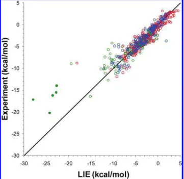
Comparison between LIE and FEP Predictions. The results of the LIE study presented here can be directly compared with those from alchemical FEP calculations of hydration free energies carried out by Mobley et al. on the same data sets and with the same force-field and charging method.16,17 One notable difference between the FEP and LIE approaches is that much shorter MD simulations in explicit solvent are required with the latter, which for the current comparison translate into at least a 1 order of magnitude speedup. This is an advantage if the increased efficiency does not compromise prediction accuracy. In Table 7, we compare the FEP predictions with LIE predictions carried out with AM1BCC-OPT partial charges and flexible solutes. We see that the LIE approach yields comparable, slightly improved predictions relative to FEP predictions in terms of MUE on the training (0.792 vs 1.095 kcal/mol), testing (0.903 vs 0.997 kcal/mol), and SAMPL1 (2.260 vs 2.594 kcal/mol) data set (SAMPL1 data set is only for 56 compounds analyzed by Mobley et al.17). A direct scatter plot between the LIE and FEP predictions is shown in Figure 5. We see that, in the case of the combined training and testing data set compounds, the LIE predictions are more negative that the FEP predictions. This change is in the correct direction since the FEP predictions for this data set were shown to be too positive relative to the experimental data.16 Indeed, for the combined training and testing data set, we obtain an MSE of 0.21 kcal/mol with the LIE method, compared to 0.68 kcal/mol afforded by the FEP data (MSEs of 0.35 kcal/mol versus 0.69 kcal/mol with the LIE versus FEP methods on the testing subset).16 In the case of the SAMPL1 data set, the LIE predictions are less negative than
the FEP predictions, whereas the latter were found to overestimate the experimental data (MSE of -1.88 kcal/mol). Thus, the LIE approach appears to at least be as accurate as the FEP approach for the prediction of hydration free energies, at a fraction of computing time. While this observation may seem counterintuitive, one possible expla-nation is that the terminal step in the alchemical transforma-tion when the solute “disappears” (λ ) 1.0 in turning off the Lennard-Jones solute-water interactions) may introduce some noise in the FEP calculations. Also, our LIE model has two fitted parameters for the cavity term, while FEP has no fitted parameters at all.
We further extended this comparison to examine whether these LIE and FEP models also perform similarly on the same functional groups. The analysis shown in Figure 6 (for raw data see Table S5), although limited to a relatively few functional groups represented by compounds containing only one type of functional group from the testing set, highlights that the LIE methods performed better on alkenes; chlori-nated, bromichlori-nated, and iodinated compounds; ethers; and nitriles, whereas the FEP method was superior on fluorinated
Table 7. Comparison of LIE and FEP Predictions of Experimental Hydration Free Energya
LIE FEP
set MUE slope R2
MUE slope R2 training 0.792 ( 0.054 0.941 ( 0.035 0.870 ( 0.025 1.095 ( 0.055 0.866 ( 0.027 0.873 ( 0.020 testing 0.903 ( 0.047 0.909 ( 0.046 0.858 ( 0.223 0.997 ( 0.040 0.936 ( 0.026 0.897 ( 0.012 SAMPL1b 2.260 ( 0.325 0.591 ( 0.047 0.821 ( 0.045 2.594 ( 0.380 0.567 ( 0.039 0.826 ( 0.051 a
LIE data are for AM1BCC-OPT charges and flexible solutes. FEP data are taken from Mobley et al.16,17Errors are in kcal mol-1units.
b
LIE and FEP data are for 56 out of the 63 compounds in the SAMPL1 data set, as in Mobley et al.17
Figure 5. Comparison between LIE predictions (this study)
and FEP predictions (Mobley et al.16,17) for the training (blue
symbols) and testing (red symbols) sets and for the SAMPL1 (green symbols) data set. Filled circles correspond to 5 sulfoneurea analogs from the SAMPL1 data set. The diagonal line indicates ideal correlation. The data correspond to MD simulations with flexible solute and AM1BCC-OPT charges, and cavity parameters derived from the training data set.
compounds, primary alcohols, neutral aliphatic amines and carboxylic acids, aldehydes, and ketones.
Decomposition into Electrostatic and Nonpolar Contributions. Free energies are often decomposed into contributions from various components. A common decom-position is into electrostatic and nonpolar contributions. In the FEP approach, this is obtained through a charge decou-pling calculation. The free energy change resulting from alchemically turning off all solute partial charges is assigned to the electrostatic contribution to hydration free energy. The nonpolar component is then obtained as the free energy change from subsequently turning off the solute-solvent Lennard-Jones interactions. However, it can be argued that this decoupling scheme does not yield a purely electrostatic contribution to the free energy because turning off the solute partial charges also results in a change in the solute-solvent van der Waals interaction energy. On the other hand, in the LIE calculation, the decomposition is somewhat cleaner. The electrostatic contribution is directly calculated from the solute-solvent Coulomb interaction energy in the presence of but not including the van der Waals interaction energy. By that we mean the configurations in the trajectory are determined by both the electrostatics and van der Waals
interactions, but the electrostatic and van der Waals contribu-tions can be formally completely separately accounted for. This distinction is important because part of the motivation for our carrying out LIE simulations on the training and testing data sets is to use the results to calibrate a new continuum solvation model. In continuum electrostatics theory, the electrostatic hydration free energy obtained from a solution of the Poisson equation (i.e., the reaction field energy) is more closely related to the LIE electrostatic decomposition than the FEP one. Hence, the LIE electrostatic decomposition is more appropriate for comparison with continuum electrostatics. Similarly, the LIE solute-solvent van der Waals energy can be used directly to calibrate a continuum van der Waals function.
A direct comparison of the electrostatic and nonpolar contributions to hydration calculated with the FEP and LIE approaches on the compounds in the training and testing data sets is given in Figure 7. While there is a good correlation between the electrostatic components from the LIE and FEP approaches, the FEP electrostatic component is systematically more positive than the LIE electrostatic component (Figure 7A). This is possibly due to the net positive change in the solute-solvent van der Waals interaction energy upon solute
Figure 6. Comparison between LIE predictions (red bars, this study) and FEP predictions (green bars, Mobley et al.16,17) for
functional classes represented by monofunctional compounds from the testing subset. The LIE data correspond to MD simulations with flexible solute and AM1BCC-OPT charges, and cavity parameters derived from the training data set. (A) MUE ( SD values. (B) MSE ( SD values.
charging, which is embedded into the FEP “electrostatic” component, although deviations from the linear response approximation may also be claimed. We have performed additional end-point calculations to quantify these effects. For 20 molecules with the largest deviations between the FEP and LIE electrostatic components (Figure 7A), we carried out MD simulations with zeroed solute charges, then recharged the solute and computed the solute electrostatic and van der Waals interactions with the nonpolarized solvent. The additional data are summarized in Table S6 (Supporting Information). Two observations stem out of these calcula-tions. First, there is very little residual electrostatic interaction
with the nonpolarized solvent, which strengthens the LIE approximation and supports the ideal theoretical value of 0.5 for the scaling of the LIE electrostatic interaction energy. Second, the difference in van der Waals interaction energy of the solute with the polarized and nonpolarized solvent compares well with the difference between the LIE and FEP electrostatic components. This supports the view that an important part of the deviation seen in Figure 7A is due to a “contamination” of the FEP electrostatic component with a positive van der Waals term incurred upon turning off the van der Waals potentials, as previously suggested by others.60,61 There is little correlation between the total nonpolar components calculated with the LIE and FEP methods (Figure 7B), due to the aforementioned formal redistribution of contributions and the narrower range of values relative to the electrostatic component.
Conclusions
The present study provides a comprehensive systematic analysis on the applicability of the LIE approach to the prediction of gas-to-water transfer free energy of small-molecule organic solutes. While the approach presented here is not new, to the best of our knowledge, this is the first theoretical analysis of hydration free energy that unifies such an extensive and diverse hydration data set comprising 564 neutral compounds with measured hydration free energies, including both “traditional” simpler compounds (the training and testing data sets) as well as more complex, drug-like compounds (the SAMPL1 data set).
Application of the LIE approach to solvation requires no empirical scaling of the solute-solvent interaction energy terms. However, a term describing the cost of cavity formation in water needs to be added to the force-field-based interaction energy terms. Using a diverse training subset that includes both polar and nonpolar solutes, we calibrated a robust linear relationship to the molecular surface area of the solute to describe the cavitation cost. On the basis of this relationship, we find that the microscopic surface tension of water is surprisingly close to the macroscopic one of 0.105 kcal mol-1Å-2. The calibrated parameters of the cavity term extend well to the compounds in the testing data sets. In agreement with other studies of solvation based on MD simulation in explicit solvent, the total nonpolar contribution to solvation calculated with the LIE method does not correlate with the solute surface area, due to a strong anticorrelation between its two main contributing factors, the cavity cost and the solute-solvent van der Waals interaction energy.
Excellent LIE models could be obtained with AM1BCC partial charges on flexible solutes in explicit water shells of 12 Å thickness and continuum models extending to infinity. These LIE models were highly correlative for the training, testing, and SAMPL1 data sets and are particularly accurate for the “traditional” compounds (MUE below 0.9 kcal/mol) and of acceptable accuracy in the case of the challenging drug-like compounds (MUE slightly above 2 kcal/mol). In the latter case, a group of sulfoneurea derivatives remain the major outliers largely responsible for the deterioration
Figure 7. Correlation between the LIE and FEP contributions
to hydration free energy. FEP data are taken from Mobley et al.16Data points for the training and testing sets are shown
with blue and red symbols, respectively. (A) Electrostatic contributions. Line indicates ideal correlation. (B) Total non-polar contributions. In the case of LIE data, the total nonnon-polar contribution includes solute-solvent van der Waals interac-tions and the cavitation cost.
in performance of the LIE model, as recently reported with most solvation methods.
We have systematically analyzed the dependence of the LIE predictions to several parameters and models, namely, continuum corrections to infinity, partial charge set, solute flexibility, and internal energy terms. Excluding the con-tinuum correction terms applied outside the explicit water shell has no impact on the LIE performance for these data sets of neutral compounds but will likely be important for solvation calculations on charged molecules. The change in the accuracy of LIE predictions with various partial charge sets is modest, with the AM1BCC-SP (without AM1 geometry optimization) charges favored over AM1BCC-OPT and RESP charges. Given its throughput and accuracy, AM1BCC-SP appears as a charging method well suited for important molecular discovery applications, such as virtual screening. The LIE predictions obtained on single-conforma-tion solutes are not much worse than those with full solute flexibility for the training and testing data sets, and somewhat to our surprise, these predictions actually improve in the case of the SAMPL1 data set. This result is extremely important for developing continuum solvation models based on explicit models. In examining the effect of including the difference in the internal energy of the solute between the solution and gas phases, we found that the inclusion of all intramolecular energy terms in the LIE model appears to be a promising approach that can lead to improved prediction accuracies. The exclusion of covalent terms yielded slightly better results over using all terms, probably due to the larger fluctuations observed for the bonded terms during the MD simulations. In an analysis of errors for a selection of functional groups represented by compounds only containing one type of functional group, we did not find any particular functional class to be a systematic major outlier. Various charge models impacted differently on the accuracy of prediction for different functional groups. For example, primary alcohols and neutral aliphatic amines had consistently underestimated hydration free energies by the LIE models with the AM1BCC partial charges, with the RESP charges having a larger improving effect for alcohols than for amines. In contrast, esters for example were only slightly overestimated with the AM1BCC charges, but RESP charges led to larger errors. A direct comparison of the LIE and alchemical FEP approaches was possible given that they were applied on the same data sets using MD simulations in explicit water with the same force field and same charging method. One notable difference between the FEP and LIE approaches is that much shorter MD simulations in explicit solvent are required with LIE over FEP, which for the current comparison translate into at least a 1 order of magnitude speedup. This speedup is a real advantage since the increased efficiency of LIE relative to FEP does not compromise prediction accuracy, and we noticed even slightly improved LIE predictions relative to FEP on both the more “traditional” training and testing data sets and the challenging drug-like SAMPL1 data set. Thus, the LIE approach appears at least as accurate as the FEP approach for predicting hydration free energies, and this at a fraction of the computing time. Finally, different free energy decomposition paths are adopted in the FEP
approach and the LIE approximation. It appears that LIE provides a simplified method for formally decomposing the solvation components that are calculated in the presence of each other. The LIE decomposition is also more compatible with the contributions to solvation that are typically calcu-lated with continuum models including Poisson electrostatics, continuum van der Waals integrals, and surface-area-based cavitation. Together with its accuracy and speed, these attributes make LIE a suitable method for calibrating a continuum solvent model that will capture the physics of the explicit-solvent model and have the required speed for accurate high-throughput applications, as we have attempted in the companion paper.35
Acknowledgment. This is National Research Council
of Canada publication number 50690.
Supporting Information Available: Composition of
the hydration data sets with experimental transfer free energies (Table S1). Composition of groups used in the functional group analysis (Table S2). LIE components to hydration free energy for all models (Table S3). Cavity parameters calibrated on the training subset for various LIE models (Table S4). Raw data from Figure 4 and 6 (Table S5). Comparison of FEP data with LIE data for polarized and nonpolarized solvent for 20 molecules from the training and testing sets (Table S6). Performance of the LIE models with flexible and single-conformation solute as a function of the number of rotatable bonds (Figure S1). This material is available free of charge via Internet at http://pubs.acs.org.
References
(1) Rashin, A. A.Prog. Biophys. Mol. Biol.1993, 60, 73–200. (2) Honig, B.; Sharp, K.; Yang, A. S.J. Phys. Chem.1993, 97,
1101–1109.
(3) Gilson, M. K.; Zhou, H. X.Annu. ReV. Biophys. Biomol. Struct.2007, 36, 21–42.
(4) Eisenberg, D.; McLachlan, A. D. Nature1986, 319, 199– 203.
(5) Kang, Y. K.; Némethy, G.; Scheraga, H. A.J. Phys. Chem.
1987, 91, 4109–4117.
(6) Sitkoff, D.; Sharp, K. A.; Honig, B.J. Phys. Chem.1994, 98, 1978–1988.
(7) Chambers, C. C.; Hawkins, G. D.; Cramer, C. J.; Truhlar, D. G.J. Phys. Chem.1996, 100, 16385–16398.
(8) Marten, B.; Kim, K.; Cortis, C.; Friesner, R. A.; Murphy, R. B.; Ringnalda, M. N.; Sitkoff, D.; Honig, B.J. Phys. Chem.
1996, 100, 11775–11788.
(9) Gallicchio, E.; Zhang, L. Y.; Levy, R. M.J. Comput. Chem.
2002, 23, 517–529.
(10) Tan, C.; Yang, L.; Luo, R. J. Phys. Chem. B 2006, 110, 18680–18687.
(11) Guthrie, J. P.J. Phys. Chem. B2009, 113, 4501–4507. (12) Mobley, D. L.; Barber, A. E.; Fennell, C. J.; Dill, K. A.J.
Phys. Chem. B2008, 112, 2405–2414.
(13) Chorny, I.; Dill, K. A.; Jacobson, M. P.J. Phys. Chem. B
2005, 109, 24056–24060.
(14) Purisima, E. O.; Sulea, T.J. Phys. Chem. B2009, 113, 8206– 8209.
(15) Reddy, M. R.; Erion, M. D. Free Energy Calculations in Rational Drug Design; Springer-Verlag: New York, 2001. (16) Mobley, D. L.; Bayly, C. I.; Cooper, M. D.; Shirts, M. R.; Dill, K. A.J. Chem. Theory Comput.2009, 5, 350–358. (17) Mobley, D. L.; Bayly, C. I.; Cooper, M. D.; Dill, K. A.J.
Phys. Chem. B2009, 113, 4533–4537.
(18) Shivakumar, D.; Deng, Y.; Roux, B. J. Chem. Theory Comput.2009, 5, 919–930.
(19) Lee, F. S.; Chu, Z. T.; Bolger, M. B.; Warshel, A.Protein Eng.1992, 5, 215–228.
(20) Aqvist, J.; Medina, C.; Samuelsson, J. E.Protein Eng.1994, 7, 385–391.
(21) Aqvist, J.; Luzhkov, V. B.; Brandsdal, B. O.Acc. Chem. Res.
2002, 35, 358–365.
(22) Aqvist, J.; Marelius, J. Comb. Chem. High Throughput Screen.2001, 4, 613–626.
(23) Jones-Hertzog, D. K.; Jorgensen, W. L.J. Med. Chem.1997, 40, 1539–1549.
(24) Su, Y.; Gallicchio, E.; Das, K.; Arnold, E.; Levy, R. M.
J. Chem. Theory Comput.2006, 3, 256–277.
(25) Wang, W.; Wang, J.; Kollman, P. A.Proteins1999, 34, 395– 402.
(26) Ben-Amotz, D.; Underwood, R.Acc. Chem. Res.2008, 41, 957–967.
(27) Carlson, H. A.; Jorgensen, W. L.J. Phys. Chem.1995, 99, 10667–10673.
(28) Almlof, M.; Carlsson, J.; Aqvist, J.J. Chem. Theory Comput.
2007, 3, 2162–2175.
(29) Mobley, D. L.; Dill, K. A.; Chodera, J. D.J. Phys. Chem. B
2008, 112, 938–946.
(30) Klamt, A.; Eckert, F.; Diedenhofen, M.J. Phys. Chem. B
2009, 113, 4508–4510.
(31) Sulea, T.; Wanapun, D.; Dennis, S.; Purisima, E. O.J. Phys. Chem. B2009, 113, 4511–4520.
(32) Nicholls, A.; Wlodek, S.; Grant, J. A.J. Phys. Chem. B2009, 113, 4521–4532.
(33) Marenich, A. V.; Cramer, C. J.; Truhlar, D. G.J. Phys. Chem. B2009, 113, 4538–4543.
(34) Soteras, I.; Forti, F.; Orozco, M.; Luque, F. J.J. Phys. Chem. B2009, 113, 9330–9334.
(35) Corbeil, C. R.; Sulea, T.; Purisima, E. O.J. Chem. Theory Comput.2010; DOI: 10.1021/ct9006037.
(36) Purisima, E. O.; Nilar, S. H.J. Comput. Chem. 1995, 16, 681–689.
(37) Purisima, E. O.J. Comput. Chem.1998, 19, 1494–1504. (38) Bhat, S.; Purisima, E. O.Proteins2006, 62, 244–261. (39) Floris, F.; Tomasi, J. J. Comput. Chem. 1989, 10, 616–
627.
(40) Floris, F. M.; Tomasi, J.; Pascual-Ahuir, J. L. J. Comput. Chem.1991, 12, 784–791.
(41) Wang, J.; Wolf, R. M.; Caldwell, J. W.; Kollman, P. A.; Case, D. A.J. Comput. Chem.2004, 25, 1157–1174.
(42) Halgren, T. A.J. Comput. Chem.1999, 20, 730–748. (43) Jakalian, A.; Bush, B. L.; Jack, D. B.; Bayly, C. I.J. Comput.
Chem.2000, 21, 132–146.
(44) Jakalian, A.; Jack, D. B.; Bayly, C. I.J. Comput. Chem.2002, 23, 1623–1641.
(45) Bayly, C. I.; Cieplak, P.; Cornell, W. D.; Kollman, P. A.J. Phys. Chem.1993, 10269–10280.
(46) Cornell, W. D.; Cieplak, P.; Bayly, C. I.; Kollman, P. A.
J. Am. Chem. Soc. 1993, 9620–9631.
(47) Schmidt, M. W.; Baldridge, K. K.; Boatz, J. A.; Elbert, S. T.; Gordon, M. S.; Jensen, J. H.; Koseki, S.; Matsunaga, N.; Nguyen, K. A.; Su, S.; Windus, T. L.; Dupuis, M.; Mont-gomery, J. A.J. Comput. Chem.1993, 14, 1347–1363. (48) Case, D. A.; Cheatham, T. E.; Darden, T.; Gohlke, H.; Luo,
R.; Merz, K. M.; Onufriev, A.; Simmerling, C.; Wang, B.; Woods, R. J.J. Comput. Chem.2005, 26, 1668–1688. (49) Wang, J.; Wang, W.; Kollman, P. A.; Case, D. A. J. Mol.
Graphics Modell.2006, 25, 247–260.
(50) Jorgensen, W. L.; Chandrasekhar, J.; Madura, J. D.; Impey, R. W.; Klein, M. L.J. Chem. Phys.1983, 79, 926–935. (51) Cornell, W. D.; Cieplak, P.; Bayly, C. I.; Gould, I. R.; Merz,
K. M.; Ferguson, D. M.; Spellmeyer, D. C.; Fox, T.; Caldwell, J. W.; Kollman, P. A.J. Am. Chem. Soc.1995, 117, 5179– 5197.
(52) Darden, T.; York, D.; Pedersen, L.J. Chem. Phys.1993, 98, 10089–10092.
(53) Ryckaert, J. P.; Ciccotti, G.; Berendsen, H. J. C.J. Comput. Phys.1977, 23, 327–341.
(54) R: A Language and EnVironment for Statistical Computing; R Foundation for Statistical Computing: Vienna, Austria, 2005.
(55) Haider, N. Checkmol. http://merian.pch.univie.ac.at/∼nhaider/ cheminf/cmmm.html (accessed March 4, 2010).
(56) Castellan, G. W. Physical Chemistry; 2nd ed.; Addison-Wesley: Reading, MA, 1971.
(57) Postma, J. P. M.; Berendsen, H. J. C.; Haak, J. R.Faraday Symp. Chem. Soc.1982, 17, 55–67.
(58) Prevost, M.; Oliveira, I. T.; Kocher, J. P.; Wodak, S. J.J. Phys. Chem.1996, 100, 2738–2743.
(59) Gasteiger, J.; Marsili, M.Tetrahedron Lett.1978, 19, 3181– 3184.
(60) Orozco, M.; Luque, F. J.Chem. Phys. Lett.1997, 265, 473– 480.
(61) Westergren, J.; Lindfors, L.; Ho¨glund, T.; Lu¨der, K.; Nord-holm, S.; Kjellander, R. J. Phys. Chem. B 2007, 111, 1872–1882.