HAL Id: hal-02500660
https://hal.inria.fr/hal-02500660
Preprint submitted on 6 Mar 2020
HAL is a multi-disciplinary open access
archive for the deposit and dissemination of
sci-entific research documents, whether they are
pub-lished or not. The documents may come from
teaching and research institutions in France or
abroad, or from public or private research centers.
L’archive ouverte pluridisciplinaire HAL, est
destinée au dépôt et à la diffusion de documents
scientifiques de niveau recherche, publiés ou non,
émanant des établissements d’enseignement et de
recherche français ou étrangers, des laboratoires
publics ou privés.
Distilled Hierarchical Neural Ensembles with Adaptive
Inference Cost
Adrià Ruiz, Jakob Verbeek
To cite this version:
Adrià Ruiz, Jakob Verbeek. Distilled Hierarchical Neural Ensembles with Adaptive Inference Cost.
2020. �hal-02500660�
Distilled Hierarchical Neural Ensembles with Adaptive Inference Cost
Adria Ruiz1 Jakob Verbeek1 2
Abstract
Deep neural networks form the basis of state-of-the-art models across a variety of application do-mains. Moreover, networks that are able to dy-namically adapt the computational cost of infer-ence are important in scenarios where the amount of compute or input data varies over time. In this paper, we propose Hierarchical Neural En-sembles (HNE), a novel framework to embed an ensemble of multiple networks by sharing inter-mediate layers using a hierarchical structure. In HNE we control the inference cost by evaluating only a subset of models, which are organized in a nested manner. Our second contribution is a novel co-distillation method to boost the performance of ensemble predictions with low inference cost. This approach leverages the nested structure of our ensembles, to optimally allocate accuracy and diversity across the ensemble members. Com-prehensive experiments over the CIFAR and Ima-geNet datasets confirm the effectiveness of HNE in building deep networks with adaptive inference cost for image classification.
1. Introduction
Deep learning models have shown impressive performance in many domains. In particular, convolutional neural net-works (CNNs) have emerged as the most successful ap-proach to solve many visual recognition tasks (Krizhevsky et al., 2012; Simonyan & Zisserman, 2014; He et al., 2016). However, state-of-the-art models typically require a large amount of computation during inference, limiting their de-ployment in edge devices such as mobile phones or au-tonomous vehicles. For this reason, methods based on net-work pruning (Huang et al., 2018b), architecture search (Tan et al., 2019), and manual network design (Sandler et al., 2018) have been proposed to learn more efficient models.
1
INRIA, Univ. Grenoble Alpes, CNRS, Grenoble INP*, LJK, 38000 Grenoble, France2Work done while at INIRA, now with Facebook AI Research. Correspondence to: Adria Ruiz <[email protected]>.
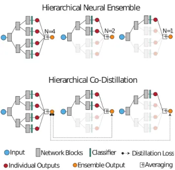
Figure 1: HNE uses a hierarchical parameter-sharing scheme generating a binary tree, where each leaf produces a separate model output. The amount of computation during inference is controlled by determining which part of the tree is evaluated for the ensemble prediction. (Bottom) Our hier-archical distillation approach leverages the full ensemble to supervise parts of the tree that are used in small ensembles.
Despite the promising results achieved by these approaches, there exist scenarios where, instead of deploying a single efficient network, we are interested in dynamically adapt-ing the inference latency dependadapt-ing on external constraints. These include situations where either the stream of data to be processed or the amount of available compute is non-constant. Examples include autonomous driving, where both might be non-constant depending on acquisition speed and the presence of other concurrent processes. Another ex-ample is scanning of incoming data streams in large online platforms such as social media networks, where the amount of traffic may surge in case of important events. Therefore, models must be able to scale the number of the operations on-the-fly depending on the amount of available compute at any point in time.
only recently started to received attention, see e.g. (Huang et al., 2018a; Yu & Huang, 2019; Ruiz & Verbeek, 2019). In this paper, we address this problem by introducing a novel framework which we refer as Hierarchical Neural Ensem-bles (HNE). Inspired by ensemble learning (Breiman, 1996), HNE embeds a large number of networks whose combined outputs provide a more accurate prediction than any indi-vidual model. In order to reduce the computational cost of evaluating multiple networks, HNE employ a binary-tree structure to share a subset of intermediate layers between the different models. Additionally, this scheme allows to control the inference cost by deciding on-the-fly how many networks to use, i.e. how many branches of the tree to eval-uate, see Figure 1 (Top). To train HNE, we also propose a novel co-distillation method adapted to the hierarchical structure of ensemble predictions, see Figure 1 (Bottom) Our contributions are summarised as follows: (i) To the best of our knowledge, we are the first to explore hierarchical ensembles for deep models with adaptive inference cost. (ii) We propose a hierarchical co-distillation scheme to increase the accuracy of ensembles for adaptive inference cost. (iii) Focusing on image classification, we show that our frame-work can be used to design efficient CNN ensembles. In particular, we evaluate the different proposed components by conducting exhaustive ablation studies on CIFAR-10/100 datasets. Additionally, compared to previous methods for adaptive inference, we show that HNE provides state-of-the-art accuracy-computation trade-offs on CIFAR-10/100 and ImageNet.
2. Related Work
Efficient networks and adaptive inference cost. Several approaches have been expored to reduce the inference cost of deep neural networks. These include the design of effi-cient convolutional blocks (Howard et al., 2017; Ma et al., 2018; Sandler et al., 2018), automated design using neural architecture search (NAS) (Wu et al., 2019; Tan et al., 2019; Cai et al., 2019), and network pruning techniques (Liu et al., 2017; Huang et al., 2018b; V´eniat & Denoyer, 2018). Whereas these approaches are effective to reduce the re-sources required by a single network, the design of models with adaptive inference cost has received less attention. To address this problem, some methods allow any-time predic-tions in DNNs by introducing intermediate classifiers pro-viding outputs at early-stages of inference (Bolukbasi et al., 2017; Huang et al., 2018a; Li et al., 2019; Elbayad et al., 2020). This idea was combined with NAS by Zhang et al. (2019) to automatically find the optimal position of the clas-sifiers. Yu & Huang (2019) and Yu et al. (2018) proposed a network that can reduce the amount of feature channels in order to adapt the computational cost. Ruiz & Verbeek (2019) introduced convolutional neural mixture models, a
probabilistic model implemented by a dense-network that can be dynamically pruned. Finally, other approaches have proposed different mechanisms to skip intermediate layers during inference in a data-dependent manner (Wu et al., 2018; Veit & Belongie, 2018; Wang et al., 2018)
Different from previous methods relying on intermediate classifiers, we address adaptive inference by exploiting hi-erarchically structured network ensembles. Additionally, our framework can be used with any base model in con-trast to other approaches which require specific network architectures (Huang et al., 2018a; Ruiz & Verbeek, 2019). Therefore, it is complementary to other works employing manual network design or NAS.
Network ensembles. Ensemble learning is a classic ap-proach to improve generalization (Hansen & Salamon, 1990; Rokach, 2010). The success of this strategy can be explained by the reduction in variance resulting from averaging the output of different learned predictors (Breiman, 1996). In the context of neural networks, seminal works (Hansen & Salamon, 1990; Krogh & Vedelsby, 1995; Naftaly et al., 1997; Zhou et al., 2002) observed that a significant accuracy boost could be achieved by averaging the outputs of inde-pendently trained models. Modern neural networks have also been shown to benefit from this strategy. In particu-lar, CNN ensembles have been employed to improve the performance of individual models (Lan et al., 2018; Lee et al., 2015), increase their robustness to label noise (Lee & Chung, 2020), and estimate outputs uncertainty (Malinin et al., 2020; Ilg et al., 2018).
The main limitation of network ensembles is the increase in training and inference costs. In practice, state-of-the-art deep models contain a large number of intermediate layers and thus, independent learning and evaluation of several networks is very costly. Whereas some strategies have been proposed to decrease the training time (Huang et al., 2017; Loshchilov & Hutter, 2017), the high inference cost still remains as a bottleneck in scenarios where computational resources are limited. In this context, different works have proposed to build ensembles where the individual networks share a subset of parameters (Lee et al., 2015; Minetto et al., 2019; Lan et al., 2018). By sharing a part of the layers between networks, the inference cost is also reduced. Our HNE uses a binary-tree structure in order to share inter-mediate layers between the individual networks. Whereas hierarchically structured networks have been explored for different purposes, such as learning mixture of experts (Liu et al., 2019; Tanno et al., 2019), incremental learning (Roy et al., 2020) or efficient ensemble implementation (Zhang et al., 2018; Lee et al., 2015), our work is the first to leverage this structure for models with adaptive inference cost. Knowledge distillation. In the context of neural networks,
knowledge distillation (KD) has been employed to improve the accuracy of a compact low-capacity “student” network, by training it on soft-labels generated by a high-capacity “teacher” network (Romero et al., 2015; Hinton et al., 2015; Ba & Caruana, 2014). However, KD has also been shown to be beneficial when the soft-labels are provided by one or multiple networks with the same architecture as the student (Furlanello et al., 2018). Another related approach is co-distillation (Zhang et al., 2018; Lan et al., 2018), where the distinction between student and teacher networks is lost and, instead, the different models are jointly optimized and distilled online. In the context of ensembles, co-distillation has been shown effective to improve the accuracy of the individual models by transferring the knowledge from the full ensemble (Anil et al., 2018; Song & Chai, 2018). In this paper, we introduce hierarchical co-distillation in order to improve the performance of HNE. Different from ensemble co-distillation strategies (Lan et al., 2018; Song & Chai, 2018), our method transfers the knowledge from the full model to smaller ensembles in a hierarchical man-ner. Previous works have also employed distillation in the context of adaptive inference (Yu & Huang, 2019; Li et al., 2019). However, our approach is specially designed for neural ensembles, where the goal is not only to improve pre-dictions requiring a low inference cost, but also to preserve the diversity between the individual network outputs.
3. Hierarchical Neural Ensemble
A hierarchical neural ensemble (HNE) embeds an ensemble of deep networks computing output yEfrom input x as:
yE= 1 N N X n=1 Fn(x; θn), (1)
where each Fnis a network with parameters θn and N is
the total number of models. In classification tasks, y ∈ RL
is a vector containing the logits for L classes. Furthermore, we assume that each network is modelled by a composition of B + 1 functions, or “blocks”:
Fn(x; θn) = fθB
n ◦ · · · ◦ fθn1 ◦ fθ0n(x), (2)
where each block fθb
n(·) is a set of layers with parameters θ.
Typically, fθb
n(·) contains a set of operations such as
convo-lutions, batch normalization layers or activation functions. Hierarchical parameter sharing. If we consider parame-ters θbnto be different for all blocks and networks, then the
complete set of model parameters is given by
Θ = {θ01:N, θ1:N1 , . . . , θ1:NB }, (3) and the inference cost of computing Eq. (1) is equivalent to evaluate N independent networks.
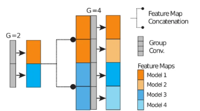
Figure 2: Efficient HNE implementation using group convo-lutions. Feature maps generated by different branches in the tree are stored in contiguous memory. Using group convolu-tions, the independent branch outputs can be computed in parallel. When a branch is split in two, the feature maps are replicated along the channel dimension and the number of groups for the next convolution is doubled.
In order to reduce the computational complexity, a HNE exploits a binary tree structure to share network parameters, where each node of the tree represents a computational block, see Figure 1. Formally, the parameters of an HNE composed of N = 2Bnetworks are collectively denoted as: Θ = {θ01, . . . , θ1:2b b, . . . , θB1:2B}, (4)
where for each block b we consider K = 2b independent
sets of parameters θb
k. This scheme generates a
hierarchi-cal structure where the number of independent parameters increases with the block index. For the first block b = 0, all the networks share θ01. For b = B there exist 2B in-dependent parameters θkBcorresponding to the number of networks in the ensemble.
Adaptive inference cost. As previously discussed, the success of ensemble learning is caused by the reduction in variance resulting from averaging a set of outputs from different models. The expected reduction in variance and improvement in accuracy are monotonic in the number of models in the ensemble. This observation allows to easily adapt the trade-off between computation and final perfor-mance. In particular, given that the different networks can be evaluated in a sequential manner, the computational cost can be controlled by choosing how many models to evaluate to approximate the ensemble prediction of Eq. (1). In the case of HNE, this can be achieved by evaluating only a sub-tree obtained by removing a set of computational blocks in the hierarchical structure, see Figure 1. More formally, we can choose any value b ∈ {0, 1, . . . , B} and compute the ensemble output using a subset of N0 = 2bnetworks as:
yb= 1 2b 2b X n=1 F (x; θn). (5)
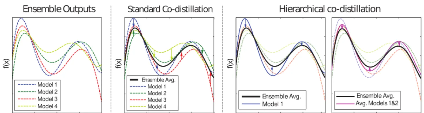
Figure 3: Comparison between standard co-distillation and our hierarchical co-distillation for ensemble learning. In the first case, the individual models are pushed to their average, reducing their variance and the overall ensemble performance. In contrast, hierarchical co-distillation preserves the model diversity by distilling smaller ensembles to the overall ensemble.
3.1. Computational Complexity
Hierarchical vs. independent networks. We analyse the inference cost of a HNE compared to an ensemble composed by fully-independent networks. By assuming that functions fbrequire the same number of operations for all blocks b,
the complexity of evaluating all the networks in a HNE is: THNE = (2B+1− 1)C, (6)
where B + 1 is the total number of blocks and C is the cost of evaluating a single function fb. Note that this quantity
is proportional to 2B+1− 1, which is the total number of
nodes in a full-binary tree of depth B.
On the other hand, it is easy to show that an ensemble composed by N networks with independent parameters has an inference cost of:
TInd= (B + 1)N C. (7)
Considering the same number of networks N = 2B in
both approaches, the ratio between the time complexities in Eq. (6) and Eq. (7) is defined by:
R = THNE TInd = 2 B + 1− 1 (B + 1)2B. (8)
For B = 0 a single network is considered, and the indepen-dent ensemble has the same computational complexity as HNE (R = 1). In contrast, when the number of evaluated models is increased (B > 0), the second term in Eq. (8) becomes negligible and the computaional complexity of a HNE is (B + 1)/2 times lower as compared to evaluating in-dependent networks. This speed-up increases linearly with the number of blocks B. This is important because, as we increase the amount of models, the ensemble accuracy is significantly improved and, therefore, it is crucial to obtain higher speed-up when evaluating large network ensembles. Efficient HNE implementation. Despite the theoretical reduction in the inference cost, a na¨ıve implementation
where the individual network outputs are computed sequen-tially does not allow to exploit the inherent parallelization power provided by modern GPUs. Fortunately, the eval-uation of the different networks in the HNE can be paral-lelized by using the notion of grouped convolutions (Xie et al., 2017; Howard et al., 2017), where different sets of input channels are used to compute an independent set of outputs. See Figure 2 for an illustration of our efficient implementation of HNE using group convolutions. 3.2. HNE Optimization
Given a training set D = {(x,y)1:M} composed of M
sample and label pairs, HNE parameters are optimized by minimizing a loss function for each individual network as:
LI(Θ) = N X n=1 M X m=1 `(F (xm; Θn), ym), (9)
where `(·, ·) is the cross-entropy loss comparing ground-truth labels with network outputs. Note that traditional ensemble methods such as bagging (Breiman, 1996), em-ploy different subsets of training data in order to increase the variance of the individual models. We do not employ this strategy here, as previous work (Neal et al., 2018; Lee et al., 2015) has shown that networks trained from different initialization already exhibit a significant diversity in their predictions. Moreover, a reduction of training samples has a negative impact on the quality of the individual models. A drawback of the loss of Eq. (9) is that it is symmetric among the networks in the ensemble. Notably, it ignores the hierarchical structure of the sub-trees that are used for adap-tive inference. To address this limitation, we can optimize a loss that measures the accuracy of the different sub-trees corresponding to the evaluation of an increasing number of
networks in the HNE: LH(Θ) = B X b=0 M X m=1 `(ybm, ym), (10) where yb
mis defined in Eq. (5). Despite the apparent
advan-tages of replacing Eq. (9) by Eq. (10) during learning, we empirically show that this strategy generally produce worse results. The reason is that Eq. (10) impedes the branches to behave as an ensemble of independent networks. Instead, the different models tend to co-adapt in order to minimize the training error and, as a consequence, averaging their outputs does not reduce the variance over test data predic-tions. In the following, we present an alternative approach that allows to effectively exploit the hierarchical structure of HNE outputs during learning.
3.3. Hierarchical Co-distillation
Previous works focused on network ensembles have ex-plored the use of co-distillation (Anil et al., 2018; Song & Chai, 2018). In particular, these methods attempt to trans-fer the ensemble knowledge to the individual models by introducing an auxiliary distillation loss for each network:
LD(Θ) = N X n=1 M X m=1 `(Fn(xm; Θn), ymE), (11) where yE
mis the ensemble output for sample xm. The
cross-entropy loss ` compares the network outputs with the soft-labels generated by normalizing yE
m. During training, the
distillation loss is combined with the standard cross-entropy loss of Eq. (9) as (1 − α)LI+ αLD, where α is an
hyper-parameter controlling the trade-off between both terms. Whereas this distillation approach boost the performance of individual models, it has a critical drawback in the context of ensemble learning for adaptive inference. In particular, standard co-distillation encourage all the predictions to be similar to their average. As a consequence, the variance between model predictions decreases, limiting the improve-ment given by combining multiple models in an ensemble. To address this limitation, we propose an novel distillation scheme which we refer to it as “hierarchical co-distillation”. The core idea is to transfer the knowledge from the full en-semble to the smaller sub-tree enen-sembles used for adaptive inference in HNE. In particular, we minimize
LHD(Θ) = B−1 X b=0 M X m=1 `(ymb , yEm). (12)
Similar to Eq. (10), the defined loss also exploits the hier-archical structure of HNE. However, in this case the pre-dictions for each sub-tree are distilled with the ensemble
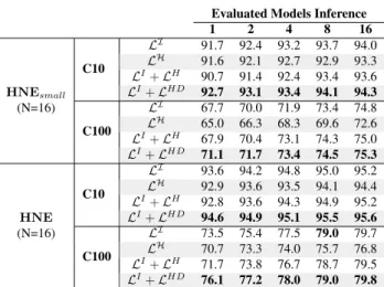
Evaluated Models Inference
1 2 4 8 16 LI 91.7 92.4 93.2 93.7 94.0 LH 91.6 92.1 92.7 92.9 93.3 LI+ LH 90.7 91.4 92.4 93.4 93.6 C10 LI+ LHD 92.7 93.1 93.4 94.1 94.3 LI 67.7 70.0 71.9 73.4 74.8 LH 65.0 66.3 68.3 69.6 72.6 LI+ LH 67.9 70.4 73.1 74.3 75.0 HNEsmall (N=16) C100 LI+ LHD 71.1 71.7 73.4 74.5 75.3 LI 93.6 94.2 94.8 95.0 95.2 LH 92.9 93.6 93.5 94.1 94.4 LI+ LH 92.8 93.6 94.3 94.9 95.2 C10 LI+ LHD 94.6 94.9 95.1 95.5 95.6 LI 73.5 75.4 77.5 79.0 79.7 LH 70.7 73.3 74.0 75.7 76.8 LI+ LH 71.7 73.8 76.7 78.7 79.5 HNE (N=16) C100 LI+ LHD 76.1 77.2 78.0 79.0 79.8 Table 1: Accuracy of HNE and HNEsmall embedding 16
different networks on CIFAR-10/100. Columns correspond to the number of models evaluated during inference.
outputs. In contrast to standard co-distillation, the minimiza-tion of Eq. (12) does not force all the models to be close to their average. As a consequence, the diversity between predictions is better preserved, retaining the advantages of averaging multiple models. See Figure 3 for an illustration.
4. Experiments
4.1. Datasets and Implementation Details
CIFAR-10/100 (Krizhevsky, 2009) contain 50k train and 10k test images from 10 and 100 classes, respectively. Following standard protocols (He et al., 2016), we pre-process the images by normalizing their mean and standard-deviation for each color channel. Additionally, during training we use a data augmentation process where we ex-tract random crops of 32×32 after applying a 4-pixel zero padding to the original image or its horizontal flip. ImageNet (Russakovsky et al., 2015) is composed by 1.2M and 50k high-resolution images for training and validation, respectively. Each sample is labelled according to 1,000 different categories. Following (Yu & Huang, 2019), we use the standard protocol during evaluation resizing the image and extracting a center crop of 224 × 224. For training, we also apply the same data augmentation process as in the cited work but remove color transformations.
Base architectures. We implement HNE with commonly used arhictectures. For CIFAR10-100, we use a variant of ResNet (He et al., 2016), composed of a sequence of residual convolutional layers with bottlenecks. We employ depth-wise instead of regular convolutions to reduce com-putational complexity. We generate a HNE with a total five blocks embedding an ensemble of N = 16 CNNs. For ImageNet, we implement an HNE based on MobileNet v2
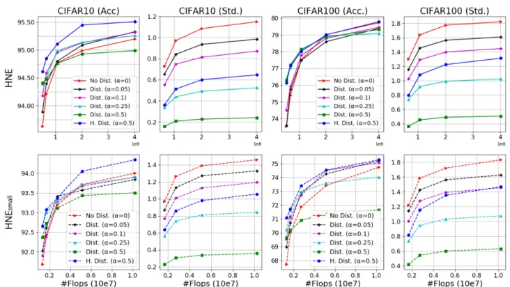
Figure 4: Accuracy and standard deviation in logits vs. FLOP count for HNE trained (i) without distillation, (ii) with standard co-distillation, and (iii) with our hierarchical co-distillation. Curves represent the evaluation of ensembles of size 1 to 16.
(Sandler et al., 2018), which uses inverted residual layers and depth-wise convolutions as main building blocks. In this case, we use four blocks generating N = 8 different networks. In supplementary material we present a detailed description of our HNE implementation using ResNet and MobileNetv2. The particular design choices for both archi-tectures are set to provide a similar computational complex-ity as previous methods to which we compare in Section 4.3. We implemented our HNE framework on Pytorch 1.0 and all the experiments are carried out over NVIDA GPUs. Our code will be released upon publication.
Inference cost metric. Following previous work (Huang et al., 2018a; Yu & Huang, 2019; Ruiz & Verbeek, 2019; Zhang et al., 2019), we evaluate the computational cost of the models according to the number of floating-point operations (FLOPs) during inference. The advantages of this metric is that it is independent from differences in hardware and implementations, and is strongly correlated with the wall-clock inference time.
Hyper-parameter settings. All the networks are opti-mized using SGD with initial learning rate of 0.1 and a momentum of 0.9. For CIFAR datasets, following Ruiz & Verbeek (2019), we train HNE using a cosine-shaped learning rate scheduler. However, for faster experimen-tation we reduce the number of epochs to 200 and use a batch size of 128. Weight decay is set to 5e−4. For
Im-ageNet, our model is trained with a cyclic learning rate schedule (Mehta et al., 2019). In particular, we use 150 epochs and reduce the learning rate with a factor two at epochs {60, 90, 110, 125, 135, 145}. We use a batch size of 450 images split across three GPUs, and weight decay is set to 1e−5. For distillation methods, following Song & Chai (2018), we use a temperature T = 2 to generate soft-labels from ensemble predictions. Finally, we set the trade-off parameter between the cross-entropy loss and the distillation loss to α = 0.5, unless specified otherwise. 4.2. Ablation Study on CIFAR-10/100
We present a comprehensive ablation study to evaluate the different components of our approach. We report results for the base ResNet architecture, as well as a version where for all layers we divided the number of feature channels by two (HNEsmall). The latter allows us to provide a more
complete evaluation by considering an additional regime where inference is extremely efficient.
Optimizing nested network ensembles. In contrast to ”single-network” learning, in HNE we are interested in op-timizing a set of ensembles generated by increasing the number of models. In order to understand the advantages of hierarchical co-distillation for this purpose, we compare four different alternative objectives that can be minimized during HNE training: (1) An independent loss for each
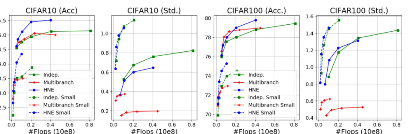
Figure 5: Results on CIFAR-10/100 using ensembles with different parameter-sharing schemes: (i) fully-independent networks, (ii) multi-branch architecture with shared backbone, (iii) the proposed hierarchical network ensemble.
model, LIin Eq. (9). (2) A hierarchical loss explicitly
max-imizing the accuracy of nested ensembles, LHin Eq. (10).
(3) A combination of both. (4) A combination of LIand the
proposed hierarchical co-distillation loss, LHDin Eq. (12).
As shown in Table 1, learning HNE with LIprovides better
performance as compared to training with LH. These results
can be understood from the perspective of the bias-variance trade-off. Concretely, note that LHattempts to reduce the
bias by co-adapting the individual outputs in order to min-imize the training error. As the different networks are not trained independently, the reduction in variance resulting from averaging multiple models in an ensemble is lost, caus-ing a performance drop on test data. This effect is also observed when combining LHwith LI. Using hierarchical
co-distillation, however, consistently outperforms the alter-natives in all the evaluated cases. Interestingly, LHD also
encourages the co-adaptation of individual outputs. How-ever, it has two critical advantages over LH. Firstly, the
co-distillation loss compares the outputs of small ensembles with a soft-label generated by averaging all the individ-ual networks. As a consequence, the matched distribution preserves the higher generalization ability produced by com-bining independent models. Secondly, as other distillation strategies, LHDis able to transfer the the information of the
logits generated by the all the models to the small ensembles. In conclusion, the presented experiment shows the benefits of our co-distillation approach to increase the accuracy of the hierarchical outputs in HNE.
Comparing distillation approaches. After demonstrating the effectiveness of hierarchical co-distillation to boost the performance of small ensembles, we evaluate its advantages w.r.t. standard co-distillation. For this purpose, we train HNE using the distillation loss of Eq. (11), as Song & Chai (2018). For standard co-distillation we also evaluate a range of values for α in order to analyze the impact on accuracy and model diversity. The latter is measured as the standard
deviation in the logits of the evaluated models, averaged across all classes and test samples. In Figure 4 we report both the accuracy on test data (Acc, in columns one and three), and standard deviation (Std, in second and fourth). From the figure we make several observations. Consider the for standard co-distillation with a high weight on the distilla-tion loss (α = 0.5). As expected, the performance of small ensembles is improved w.r.t. training without distillation. For larger ensembles, however, the accuracy tends to be sig-nificantly lower compared not using distillation, due to the reduction in diversity among the models induced by the co-distillation loss. This effect can be controlled by reducing the weight α of the distillation loss, but smaller values for α tend to compromise the accuracy of small ensembles. In con-trast, our hierarchical co-distillation achieves comparable or better performance for all ensemble sizes and datasets. For small ensemble sizes, we obtain improvements over training without distillation that are either comparable or larger than the ones obtained with standard co-distillation. For large ensemble sizes, our approach significantly improves over standard co-distillation, and the accuracy is comparable if not better for large ensembles obtained without distillation. In Supplementary Material we provide additional results to give more insights on the advantages of hierarchical co-distillation for HNE.
Hierarchical parameter sharing. In this experiment, we compare the performance obtained by HNE and an ensemble of independent networks that are not organized in a tree structure, using the same base architecture. We also compare to the multi-branch architecture explored by Lan et al. (2018) and Lee et al. (2015). In this case, the complexity is reduced by sharing the same “backbone” for the first blocks for all models, and then bifurcate to N independent branches for the subsequent blocks. For HNE we use five different blocks with N = 16. To achieve architectures in a similar FLOP range, we use the first three blocks as the backbone and
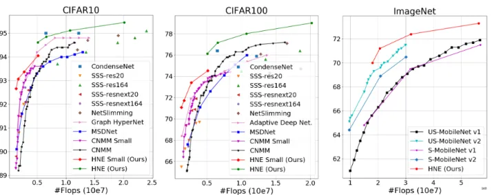
Figure 6: Comparison of HNE with the state of the art. Curves correspond to results obtained by models with adaptive inference cost. Disconnected points show results for methods requiring independent models for each FLOP count.
implement 16 independent branches for the last two blocks. We use hierarchical distillation for all three architectures. In Figure 5 we again report both the accuracy (Acc) and the standard deviation of logits (Std).
From the results, we observe that HNE obtains significantly better results than the independent networks. Moreover, the hierarchical structure allows to significantly reduce the computational cost for large ensemble sizes. The multi-branch scheme achieves slightly better performance when the amount of evaluated models is small, but HNE is signifi-cantly better for larger ensembles. These results can again be understood by observing the diversity across models. In particular, we see that sharing a common backbone for all networks drastically reduces diversity in predictions. In con-trast, HNE leads to prediction diversity that is comparable to that of independent networks that do not share any param-eters or computations. This shows the importance of using independent sets of parameters in early-blocks to achieve diversity between individual models.
4.3. Comparison with the state of the art
CIFAR-10/100. We compare the performance of HNE trained with hierarchical co-distillation with previous ap-proaches proposed for learning CNNs with adaptive infer-ence cost: Multi-scale DenseNet (Huang et al., 2018a), Graph Hyper-Networks (Zhang et al., 2019), Deep Adaptive Networks (Li et al., 2019), and Convolutional Neural Mix-ture Models (Ruiz & Verbeek, 2019). Following (Ruiz & Verbeek, 2019), we also show the results obtained by previ-ous network pruning methods used to reduce the inference cost in CNNs: NetSlimming (Liu et al., 2017), CondenseNet (Huang et al., 2018b), and SSS (Huang & Wang, 2018). We report HNE result for ensembles of sizes up to eight, in order
to provide a maximum FLOP count similar to the compared methods (<250M).
Results in Figure 6 show that for both datasets HNE consis-tently outperforms previous approaches with adaptive com-putational complexity. Considering also network pruning methods, only CondenseNet obtains a small improvement on CIFAR10 for a single operating point. This approach, however, requires to train and evaluate a separate model to achieve any particular inference cost.
ImageNet. We compare our method with slimmable (Yu et al., 2018), and universally slimmable Networks (Yu & Huang, 2019). To the best of our knowledge these works have reported state-of-the-art performance on ImageNet for adaptive CNNs with a relatively low computational com-plexity. In particular, we report results obtained with a similar inference cost range than our HNE based on Mo-bileNetv2 architecture (∼150-600M FLOPs). For hierarchi-cal co-distillation we use α = 0.75.
The results in Figure 6 show that our HNE achieves better accuracy than the compared methods across all inference cost levels. Moreover, our approach is complementary to slimmable networks as the dynamic reduction in feature channels used in slimmable networks can be applied to the blocks in our hierarchical structure. Combining HNE with this strategy provides a complementary mechanism to find better trade-offs between computation and accuracy.
5. Conclusions
We have proposed Hierarchical Neural Ensembles (HNE), a framework to design deep models with adaptive inference cost. Additionally, we have introduced a novel hierarchical
co-distillation approach adapted to the structure of HNE. Compared to previous methods for adaptive deep networks, we have reported state-of-the-art compute-accuracy trade-offs on CIFAR-10/100 and ImageNet.
While we have demonstrated the effectiveness of our frame-work in the context of CNNs for image classification, our approach is generic and can be used to build ensembles of other types of deep networks for different tasks and do-mains, for example in NLP. Our framework is complemen-tary to network compression and neural architecture search methods. We believe that a promising line of research for adaptive models is to explore the combination of these type of approaches with our hierarchical neural ensembles. ACKNOWLEDGMENTS
This work has been partially supported by the grant “Deep in France” (ANR-16-CE23-0006).
References
Anil, R., Pereyra, G., Passos, A., Ormandi, R., Dahl, G. E., and Hinton, G. E. Large scale distributed neural network training through online distillation. ICLR, 2018. Ba, J. and Caruana, R. Do deep nets really need to be deep?
In NIPS, 2014.
Bolukbasi, T., Wang, J., Dekel, O., and Saligrama, V. Adap-tive neural networks for efficient inference. In ICML, 2017.
Breiman, L. Bagging predictors. Machine learning, 1996. Cai, H., Zhu, L., and Han, S. ProxylessNAS: Direct neural
architecture search on target task and hardware. ICLR, 2019.
Elbayad, M., Gu, J., Grave, E., and Auli, M. Depth-adaptive transformer. In ICLR, 2020.
Furlanello, T., Lipton, Z. C., Tschannen, M., Itti, L., and Anandkumar, A. Born again neural networks. In ICML, 2018.
Hansen, L. and Salamon, P. Neural network ensembles. PAMI, 12(10), 1990.
He, K., Zhang, X., Ren, S., and Sun, J. Deep residual learning for image recognition. In CVPR, 2016.
Hinton, G., Vinyals, O., and Dean, J. Distilling the knowledge in a neural network. arXiv preprint arXiv:1503.02531, 2015.
Howard, A., Sandler, M., Chu, G., Chen, L.-C., Chen, B., Tan, M., Wang, W., Zhu, Y., Pang, R., Vasudevan, V., et al. Searching for mobilenetv3. In ICCV, 2019.
Howard, A. G., Zhu, M., Chen, B., Kalenichenko, D., Wang, W., Weyand, T., Andreetto, M., and Adam, H. Mobilenets: Efficient convolutional neural networks for mobile vision applications. arXiv preprint arXiv:1704.04861, 2017. Huang, G., Li, Y., Pleiss, G., Liu, Z., Hopcroft, J. E., and
Weinberger, K. Q. Snapshot ensembles: Train 1, get m for free. ICLR, 2017.
Huang, G., Chen, D., Li, T., Wu, F., van der Maaten, L., and Weinberger, K. Q. Multi-scale dense networks for resource efficient image classification. ICLR, 2018a. Huang, G., Liu, S., van der Maaten, L., and Weinberger, K.
CondenseNet: An efficient densenet using learned group convolutions. In CVPR, 2018b.
Huang, Z. and Wang, N. Data-driven sparse structure selec-tion for deep neural networks. In ECCV, 2018.
Ilg, E., Cicek, O., Galesso, S., Klein, A., Makansi, O., Hutter, F., and Brox, T. Uncertainty estimates and multi-hypotheses networks for optical flow. In ECCV, 2018. Krizhevsky, A. Learning multiple layers of features from
tiny images. Master’s thesis, University of Toronto, 2009. Krizhevsky, A., Sutskever, I., and Hinton, G. ImageNet
classification with deep convolutional neural networks. In NIPS, 2012.
Krogh, A. and Vedelsby, J. Neural network ensembles, cross validation, and active learning. In NIPS, 1995.
Lan, X., Zhu, X., and Gong, S. Knowledge distillation by on-the-fly native ensemble. In NIPS, 2018.
Lee, J. and Chung, S.-Y. Robust training with ensemble consensus. In ICLR, 2020.
Lee, S., Purushwalkam, S., Cogswell, M., Crandall, D., and Batra, D. Why m heads are better than one: Training a diverse ensemble of deep networks. arXiv preprint arXiv:1511.06314, 2015.
Li, H., Zhang, H., Qi, X., Yang, R., and Huang, G. Improved techniques for training adaptive deep networks. In ICCV, 2019.
Liu, Y., Stehouwer, J., Jourabloo, A., and Liu, X. Deep tree learning for zero-shot face anti-spoofing. In CVPR, 2019. Liu, Z., Li, J., Shen, Z., Huang, G., Yan, S., and Zhang, C. Learning efficient convolutional networks through network slimming. In ICCV, 2017.
Loshchilov, I. and Hutter, F. Sgdr: Stochastic gradient descent with warm restarts. In ICLR, 2017.
Ma, N., Zhang, X., Zheng, H.-T., and Sun, J. ShuffleNet V2: Practical guidelines for efficient CNN architecture design. In ECCV, 2018.
Malinin, A., Mlodozeniec, B., and Gales, M. Ensemble distribution distillation. In ICLR, 2020.
Mehta, S., Rastegari, M., Shapiro, L., and Hajishirzi, H. Espnetv2: A light-weight, power efficient, and general purpose convolutional neural network. CVPR, 2019. Minetto, R., Segundo, M., and Sarkar, S. Hydra: an
en-semble of convolutional neural networks for geospatial land classification. IEEE Transactions on Geoscience and Remote Sensing, 2019.
Naftaly, U., Intrator, N., and Horn, D. Optimal ensemble averaging of neural networks. Network: Computation in Neural Systems, 1997.
Neal, B., Mittal, S., Baratin, A., Tantia, V., Scicluna, M., Lacoste-Julien, S., and Mitliagkas, I. A modern take on the bias-variance tradeoff in neural networks. arXiv preprint arXiv:1810.08591, 2018.
Rokach, L. Ensemble-based classifiers. Artificial Intelli-gence Review, 2010.
Romero, A., Ballas, N., Kahou, S. E., Chassang, A., Gatta, C., and Bengio, Y. Fitnets: Hints for thin deep nets. ICLR, 2015.
Roy, D., Panda, P., and Roy, K. Tree-CNN: a hierarchi-cal deep convolutional neural network for incremental learning. Neural Networks, 2020.
Ruiz, A. and Verbeek, J. Adaptative inference cost with convolutional neural mixture models. In ICCV, 2019. Russakovsky, O., Deng, J., Su, H., Krause, J., Satheesh, S.,
Ma, S., Huang, Z., Karpathy, A., Khosla, A., Bernstein, M., Berg, A. C., and Fei-Fei, L. ImageNet large scale visual recognition challenge. IJCV, 2015.
Sandler, M., Howard, A., Zhu, M., Zhmoginov, A., and Chen, L.-C. MobileNetV2: Inverted residuals and linear bottlenecks. In CVPR, 2018.
Simonyan, K. and Zisserman, A. Very deep convolutional networks for large-scale image recognition. BMVC, 2014. Song, G. and Chai, W. Collaborative learning for deep
neural networks. In NIPS, 2018.
Tan, M., Chen, B., Pang, R., Vasudevan, V., Sandler, M., Howard, A., and Le, Q. MnasNet: Platform-aware neural architecture search for mobile. In CVPR, 2019.
Tanno, R., Arulkumaran, K., Alexander, D., Criminisi, A., and Nori, A. Adaptive neural trees. ICML, 2019.
Veit, A. and Belongie, S. Convolutional networks with adaptive inference graphs. In ECCV, 2018.
V´eniat, T. and Denoyer, L. Learning time/memory-efficient deep architectures with budgeted super networks. In CVPR, 2018.
Wang, X., Yu, F., Dou, Z.-Y., Darrell, T., and Gonzalez, J. E. SkipNet: Learning dynamic routing in convolutional networks. In ECCV, 2018.
Wu, B., Dai, X., Zhang, P., Wang, Y., Sun, F., Wu, Y., Tian, Y., Vajda, P., Jia, Y., and Keutzer, K. FBNet: Hardware-aware efficient convnet design via differentiable neural architecture search. In CVPR, 2019.
Wu, Z., Nagarajan, T., Kumar, A., Rennie, S., Davis, L., Grauman, K., and Feris, R. BlockDrop: Dynamic infer-ence paths in residual networks. In CVPR, 2018. Xie, S., Girshick, R., Doll´ar, P., Tu, Z., and He, K.
Aggre-gated residual transformations for deep neural networks. In CVPR, 2017.
Yu, J. and Huang, T. Universally slimmable networks and improved training techniques. ICCV, 2019.
Yu, J., Yang, L., Xu, N., Yang, J., and Huang, T. Slimmable neural networks. ICLR, 2018.
Zhang, C., Ren, M., and Urtasun, R. Graph hypernetworks for neural architecture search. ICLR, 2019.
Zhang, Y., Xiang, T., Hospedales, T. M., and Lu, H. Deep mutual learning. In CVPR, 2018.
Zhou, Z.-H., Wu, J., and Tang, W. Ensembling neural networks: many could be better than all. Artificial intelli-gence, 2002.
Supplementary Material
A. HNE Architectures
In the following, we provide a detailed description of our HNE implementation using ResNet (He et al., 2016) and MobileNetV2 (Sandler et al., 2018) architectures for the CIFAR and ImageNet datasets, respectively.
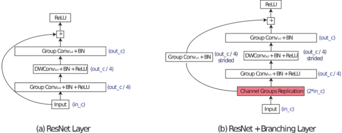
ResNet HNE. We build our HNE using the two types of layers illustrated in Figure 7. We refer to them as ResNet and ResNet+Branching. The first one implements a standard residual block with bottleneck (He et al., 2016). However, as described in Figure 2 of the main paper, we replace standard convolutional filters by group convolutions in order to compute in parallel the output of the different branches in the tree structure. Additionally, we also replace the standard 3 × 3 convolution by a depth-wise separable 3 × 3 convolution (Howard et al., 2017) in order to reduce computational complexity. The ResNet+Branching layer follows the structure of ResNets ”shortcut” blocks used when the image resolution is reduced or the number of channels is augmented. In HNE we employ it when a branch is split in two. Therefore, we add a channel replication operation as shown in Figure 7(b). Using these two types of layers, we implement HNE with B = 5 blocks embedding a total of 16 ResNets of depth 50. See Table 2 for a detailed description of the full architecture configuration.
Figure 7: The two layers used in HNE with ResNet architecture. We use in c and out c to refer to the number of input and output feature channels of the convolutional block as described in Table 2. In blue, we show the number of channels resulting after applying each block and whether strided convolution is used or not. BN refers to Batch Normalization.
Block. Index
Layer
Type Stride Repetitions
Input Res. Output Res. Input Groups (Gi) Output Groups (Go) Input Channels Output Channels 0 Conv3×3+ BN + ReLU 1 1 32 × 32 32 × 32 1 1 3 16 0 Conv1×1+ BN + ReLU 1 1 32 × 32 32 × 32 1 1 16 64 1 ResNet+Branching 1 1 32 × 32 32 × 32 1 2 64 64 Go 1 ResNet 1 2 32 × 32 32 × 32 2 2 64 Gi 64 Go 2 ResNet+Branching 2 1 32 × 32 16 × 16 2 4 64 Gi 128 Go 2 ResNet 1 3 16 × 16 16 × 16 4 4 128 Gi 128 Go 3 ResNet+Branching 2 1 16 × 16 8 × 8 4 8 128 Gi 256 Go 3 ResNet 1 3 8 × 8 8 × 8 8 8 256 Gi 256 Go 4 ResNet+Branching 2 1 8 × 8 8 × 8 8 16 256 Gi 256 Go 4 ResNet 1 4 8 × 8 8 × 8 16 16 256 Gi 256 Go
Classifier Avg. Pool + Linear 1 1 8 × 8 1 × 1 16 16 256 Gi L Go
Table 2: Full layer configuration of HNE based on ResNet architecture. Each row shows: (1) The block index in the hierarchical structure. (2) The type of layer, whether strided convolutions is used and the number of times that it is stacked. (3) Input and output resolutions of the feature maps. (4) The number of input and output groups used for convolutions, representing the number of active branches in the tree structure. (5) The number of input and output channels before and after applying the layers. Note that it is multiplied by the number of input and output groups representing the number of active branches. Finally, L refers to the number of classes in the dataset.
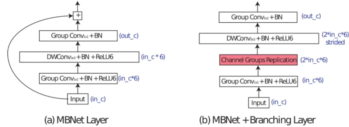
MobileNet HNE. In order to implement an efficient ensemble of MobileNetV2 networks, we employ the same layers used in the original architecture (see Figure 8). In this case, we refer to them as MBNet and MBNet+Branching layers. The first one implements the inverted residual blocks used in MobileNetV2 but using group convolutions to account for the different HNE branches. The second one is analogous to the shortcut blocks used in this model but we add a channel group replication to implement the branch splits in the tree structure. The detailed layer configuration is shown in Table 3. Note that our MobileNet HNE embed a total of 8 networks with the same architecture as a MobileNetV2 model with channel width multiplier of 0.75. The only difference is that we replace the last convolutional layer by a 1 × 1 convolution and a fully-connected layer, as suggested in (Howard et al., 2019). This modification offers a reduction of the total number of FLOPs without a significant drop in accuracy.
Figure 8: The two layers used in HNE with MobileNet architectures. We use in c and out c to refer to the number of input and output feature channels of the convolutional block as described in Table 3. In blue, we show the number of channels resulting after applying each block and whether strided convolution is used. BN refers to Batch Normalization.
Block. Index
Layer
Type Stride Repetitions
Input Res. Output Res. Input Groups (Gi) Output Groups (Go) Input Channels Output Channels 0 Conv3×3+ BN + ReLU6 2 1 224 × 224 112 × 112 1 1 3 16 0 Conv1×1+ BN + ReLU6 1 1 112 × 112 112 × 112 1 1 16 16 0 MBNet 2 2 112 × 112 56 × 56 1 1 16 24 1 MBNet+Branching 2 1 56 × 56 28 × 28 1 2 24 24 Go 1 MBNet 1 2 28 × 28 28 × 28 2 2 24 Gi 24 Go 2 MBNet+Branching 2 1 28 × 28 14 × 14 2 4 24 Gi 48 Go 2 MBNet 1 3 14 × 14 14 × 14 4 4 48 Gi 48 Go 2 MBNet 1 3 14 × 14 14 × 14 4 4 48 Gi 72 Go 3 MBNet+Branching 2 1 14 × 14 7 × 7 4 8 72 Gi 120 Go 3 MBNet 1 2 7 × 7 7 × 7 8 8 120 Gi 120 Go 3 Conv1×1+ BN + ReLU6 1 1 7 × 7 7 × 7 8 8 120 Gi 720 Go
3 Avg. Pool + Linear + ReLU6 1 1 7 × 7 1 × 1 8 8 720 Gi 1280 Go
Classifier Linear 1 1 1 × 1 1 × 1 8 8 1280 Gi 1000 Go
Table 3: Full layer configuration of HNE based on MobileNetV2 architecture. Each row shows: (1) The block index in the hierarchical structure. (2) The type of layer, whether strided convolutions is used and the number of times that it is stacked. (3) Input and output resolutions of the feature maps. (4) The number of input and output groups used for convolutions, representing the number of active branches in the tree structure. (5) The number of input and output channels before and after applying the layers. Note that it is multiplied by the number of input and output groups representing the number of active branches.
B. Additional Results on Hierarchical Co-distillation
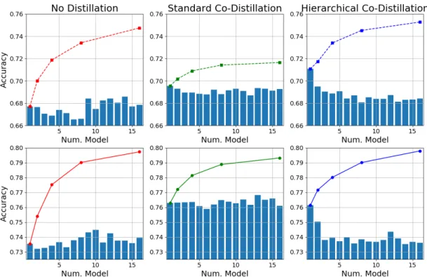
We provide additional results to give more insights on the effect of the evaluated distillation approaches. Figure 9 depicts the performance of HNE for a different ensemble sizes used during inference (curves) and the accuracy of the individual networks in the ensemble (bars). Comparing the results without distillation to standard co-distillation, we can observe that the latter significantly increases the accuracy of the individual models. This is expected because the knowledge from the complete ensemble is transferred to each network independently. However, the accuracy when the number of evaluated models is increased tend to be lower than HNE trained without distillation. Despite the fact that both phenomena may seem counter-intuitive, they can be explained because standard co-distillation tend to decrease the diversity between the individual models. As a consequence, the gains obtained by combining a large number of networks is reduced even though they are individually more accurate.
The reported results for Hierarchical Co-Distillation clearly show its advantages with respect to the alternative approaches. In this case, we can observe that the accuracy of the first model is much higher than in HNE trained without distillation, and similar to the model obtained by standard co-distillation. The reason is that the ensemble knowledge is directly transferred to the predictions of the first network in the hierarchical structure. Additionally, the performance of the rest of networks is usually lower than HNE trained with standard co-distillation. The improvement obtained by ensembling their predictions is, however, significantly higher. As discussed in the main paper, this is because hierarchical co-distilllation preserves the diversity between the network outputs better, even though their individual average performance can be worse.
Figure 9: Results on CIFAR100 for HNEsmall(top) and HNE (botton) trained without distillation, standard co-distillation
and the proposed hierarchical co-distillation. Curves indicate the performance of the different ensembles when the number of evaluated models is increased. Bars depict the accuracy of each individual network.