HAL Id: inria-00381582
https://hal.inria.fr/inria-00381582
Submitted on 5 May 2009
HAL is a multi-disciplinary open access
archive for the deposit and dissemination of
sci-entific research documents, whether they are
pub-lished or not. The documents may come from
teaching and research institutions in France or
abroad, or from public or private research centers.
L’archive ouverte pluridisciplinaire HAL, est
destinée au dépôt et à la diffusion de documents
scientifiques de niveau recherche, publiés ou non,
émanant des établissements d’enseignement et de
recherche français ou étrangers, des laboratoires
publics ou privés.
Self-stabilizing Deterministic Gathering
Yoann Dieudonné, Franck Petit
To cite this version:
Yoann Dieudonné, Franck Petit. Self-stabilizing Deterministic Gathering. [Research Report] 2009.
�inria-00381582�
Self-stabilizing Deterministic Gathering
Yoann Dieudonn´e1 Franck Petit2
1 MIS CNRS, Universit´e de Picardie Jules Verne Amiens, France 2 INRIA, LIP UMR 5668, Universit´e de Lyon / ENS Lyon, France
Abstract. In this paper, we investigate the possibility to deterministi-cally solve the gathering problem (GP) with weak robots (anonymous, autonomous, disoriented, deaf and dumb, and oblivious). We introduce strong multiplicity detection as the ability for the robots to detect the exact number of robots located at a given position. We show that with strong multiplicity detection, there exists a deterministic self-stabilizing algorithm solving GP for n robots if, and only if, n is odd.
Keywords: Distributed Coordination, Gathering, Mobile Robot Net-works, Self-stabilization.
1
Introduction
The distributed systems considered in this paper are teams (or swarms) of mobile robots (sensors or agents). Such systems supply the ability to collect (to sense) environmental data such as temperature, sound, vibration, pressure, motion, etc. The robots use these sensory data as an input in order to act in a given (sometimes dangerous) physical environment. Numerous potential applications exist for such multi-robot systems, e.g., environmental monitoring, large-scale construction, risky area surrounding, exploration of an unknown area. All these applications involve basic cooperative tasks such as pattern formation, gathering, scatter, leader election, flocking, etc.
Among the above fundamental coordination tasks, we address the gathering (or Rendez-Vous) problem. This problem can be stated as follows: robots, ini-tially located at various positions, gather at the same position in finite time and remain at this position thereafter. The difficulty to solve this problem greatly de-pends on the system settings, e.g., whether the robots can remember past events or not, their means of communication, their ability to share a global property like observable IDs, sense of direction, global coordinate, etc. For instance, assuming that the robots share a common global coordinate system or have (observable) IDs allowing to differentiate any of them, it is easy to come up with a deter-ministic distributed algorithm for that problem. Gathering turns out to be very difficult to solve with weak robots, i.e., devoid of (1) any (observable) IDs al-lowing to differentiate any of them (anonymous), (2) any central coordination mechanism or scheduler (autonomous), (3) any common coordinate mechanism or common sense of direction (disoriented), (4) means of communication allow-ing them to communicate directly, e.g., by radio frequency (deaf and dumb), and (5) any way to remember any previous observation nor computation performed
in any previous step (oblivious). Every movement made by a robot is then the result of a computation having observed positions of the other robots as a only possible input. With such settings, assuming that robots are points evolving on the plane, no solution exists for the gathering problem if the system contains two robots only [19]. It is also shown in [15] that gathering can be solved only if the robots have the capability to know whether several robots are located at the same position (multiplicity detection). Note that a strong form of such an ability is that the robot are able to count the exact number of robots located at the same position. A weaker form consists in considering the detector as an abstract device able to say if any robot location contains either exactly one or more than one robot.
In this paper, we investigate the possibility to deterministically solve the gathering problem with weak robots (i.e., anonymous, autonomous, disoriented, deaf and dumb, and oblivious). This problem has been extensively studied in the literature assuming various settings. For instance, the robots move either among the nodes of a graph [11,13], or in the plane [1,2,4,12,14,15,19], their visibility can be limited (visibility sensors are supposed to be accurate within a constant range, and sense nothing beyond this range) [12,17], robots are prone to faults [1,7].
In this paper, we address the stabilization aspect of the gathering problem. A deterministic system is (self-)stabilizing if, regardless of the initial states of the computing units, it is guaranteed to converge to the intended behavior in a finite number of steps [9]. To our best knowledge, all the above solutions assume that in the initial configuration, no two robots are located at the same position. So, effectively, as already noticed in [6,8], this implies that none of them is “truly” self-stabilizing—initial configurations where robots are located at the same positions are avoided. Note that surprisingly, such an assumption prevents to initiate the system where the problem is solved, i.e., initially all the robots occupy the same position.
In this paper, we study the gathering problem assuming any arbitrary ini-tial configurations, that is in which some robots can share the same positions. Clearly, assuming weak multiplicity detection (each robot location contains ei-ther exactly one or more than one robot), the problem cannot be solved de-terministically. Informally, if all the robots are at exactly two positions, then there is no way to maintain a particular position as an invariant. So, there are some executions where the system behaves as if it contains exactly two robots, leading to the impossibility result in [19]. We introduce the concept of strong multiplicity detection—the robot are able to count the exact number of robots located at the same position. Even with such capability, the problem cannot be solved deterministically, if the number of robots is even. The proof is similar as above: If initially the robots occupy exactly two positions, then there is no way to maintain a particular position as an invariant. Again, the impossibility result in [19] holds. By contrast, we show that with an odd number of robots, the problem is solvable. Our proof is constructive, as we present and prove a
deterministic algorithm for that problem. The proposed solution has the nice property of being self-stabilizing since no initial configuration is excluded.
In the next section (Section 2), we describe the distributed system and the problem we consider in this paper. Our main result with its proof is given in Section 3. We conclude this paper in Section 4. Due to the lack of space, some proofs have been moved in the Annexes section.
2
Preliminaries
In this section, we define the distributed system and the problem considered in this paper.
2.1 Distributed Model.
We adopt the semi-synchoronous model introduced in [18], below referred to as SSM . The distributed system considered in this paper consists of n robots r1, r2,· · · , rn—the subscripts 1, . . . , n are used for notational purpose only. Each
robot ri, viewed as a point in the Euclidean plane, moves on this two-dimensional
space unbounded and devoid of any landmark. It is assumed that two or more robots may simultaneously occupy the same physical location.
Any robot can observe, compute and move with infinite decimal precision. The robots are equipped with sensors enabling to detect the instantaneous po-sition of the other robots in the plane. In particular, we distinguish two types of multiplicity detection : weak multiplicity detection and strong multiplicity
de-tection.
Definition 1 (Weak multiplicity detection). [4,10] The robots have weak
multiplicity detection if, for every point p, their sensors can detect if there is no robot, there is one robot, or there are more than one robot. In the latter case, the robot might not be capable of determining the exact number of robots.
Definition 2 (Strong multiplicity detection). The robots have strong
mul-tiplicity detection if, for every point p, their sensors can detect the number of robots on p.
Each robot has its own local coordinate system and unit measure. The robots do not agree on the orientation of the axes of their local coordinate system, nor on the unit measure. They are uniform and anonymous, i.e, they all have the same program using no local parameter (such that an identity) allowing to differentiate any of them. They communicate only by observing the position of the others and they are oblivious, i.e., none of them can remember any previous observation nor computation performed in any previous step.
Time is represented as an infinite sequence of time instants 0, 1, . . . , j, . . . Let P(t) be the set of the positions in the plane occupied by the n robots at time t. For every t, P(t) is called the configuration of the distributed system in t. Given any point p, |p| denotes the number of robots located on p. Note that, if the
robots do not have the multiplicity detection then |p| ≤ 1 for all the robots. P(t) expressed in the local coordinate system of any robot ri is called a view.At each
time instant t, each robot ri is either active or inactive. The former means that,
during the computation step (t, t + 1), using a given algorithm, ri computes in
its local coordinate system a position pi(t + 1) depending only on the system
configuration at t, and moves towards pi(t + 1)—pi(t + 1) can be equal to pi(t),
making the location of ri unchanged. In the latter case, ridoes not perform any
local computation and remains at the same position. In every single activation, the distance traveled by any robot r is bounded by σr. So, if the destination
point computed by r is farther than σr, then r moves toward a point of at most
σr. This distance may be different between two robots.
The concurrent activation of robots is modeled by the interleaving model in which the robot activations are driven by a fair scheduler. At each instant t, the scheduler arbitrarily activates a (non empty) set of robots. Fairness means that every robot is infinitely often activated by the scheduler.
2.2 Specification
The Gathering Problem (GP) is to design a distributed protocol P for n mobile robots so that the following properties are true :
– Convergence: Regardless of the initial positions of the robots on the plane, all the robots are located at the same position in finite time.
– Closure: Starting from a configuration where all the robots are located at the same position, all the robots are located at the same position thereafter.
3
Gathering with strong multiplicity detection
In this section, we prove the following theorem :
Theorem 1. With strong multiplicity detection, there exists a deterministic
self-stabilizing algorithm solving GP for n robots if, and only if, n is odd.
As mentionned in the introduction, even with strong multiplicity detection there do not exist any deterministic algorithm solving GP for an even number of robots. So, to prove Theorem 1 we first give a deterministic self-stabilizing algorithm solving GP for an odd number of robots having the strong multiplicity detection. Then, we prove the correctness of the algorithm.
3.1 Deterministic Self-stabilizing Algorithm for an odd number of robots.
In this subsection, we give a deterministic self-stabilizing algorithm solving GP for an odd number of robots. We first provide particular notations, basic defi-nitions and properties that we use for symplifying the design and proofs of the protocol. Next, the protocol is presented.
Notations, Basic Definitions and Properties. Given a configuration P, M axP indicates the set of all the points p such that |p| is maximal. In other terms, ∀pi ∈ M axP and ∀pj ∈ P, we have |pi| ≥ |pj|. |M axP| will be the
cardinality of M axP.
Remark 1. Since the robots have the strong multiplicity detection, then they
are able to compute |p| for every point p ∈ P. In particular, all the robots can determine M axP(t) at each time instant t.
Given three distinct points r, r′ and c in the plane, we say that the two
half-lines [c, r) and [c, r′) divide the plane into two sectors if and only if
– either r, r′ and c are not colinear,
– or r, r′ and c are colinear and c is between r and r′ on the segment [r, r′].
If it exists then this pair of sectors is denoted by {rcr′, rcr′} and we assume
that the two half-lines [c, r) and [c, r′) do not belong to any sector in {rcr′, rcr′}
. Note that, if the three points r, r′and c are not colinear then one of two sectors
is convex (angle centered at c between r and r′ ≤ 180o) and the other one is
concave (angle centered at c between r and r′ > 180o). Otherwise, the three
points r, r′ and c are colinear and the two sectors are convex and more precisely
they are straight (both conjugate angles centered at c between r and r′are equal
to 180o).
Definition 3 (Smallest enclosing circle). [6] Given a set P of n ≥ 2 points p1, p2,· · · , pn on the plane, the smallest enclosing circle of P , called SEC(P), is
the smallest circle enclosing all the positions in P. It passes either through two of the positions that are on the same diameter (opposite positions), or through at least three of the positions in P.
When no ambiguity arises, SEC(P) will be shortly denoted by SEC and SEC(P) ∩ P will indicate the set of all the points both on SEC(P) and P. Besides, we will say that a robot r is inside SEC if, and only if, there is not located on the circumference of SEC. In any configuration P, SEC is unique and can be computed in linear time [3].
Given a set P of n ≥ 2 points p1, p2,· · · , pn on the plane and SEC(P) its
smallest enclosing circle, Rad(SEC(P)) will indicate the length of the radius of SEC(P).
The next lemma contains a simple fact.
Lemma 1. Let P1 be an arbitrary configuration of n points. Let P2 be a con-figuration obtained by pushing inside SEC(P1) all the points which are in P1∩ SEC(P1). We have Rad(SEC(P2)) < Rad(SEC(P1)).
Let S and C be respectively a sector in {pcp′, pcp′} and a circle centered
at c. We denote by arc(C, S) the arc of the circle C inside S. Given a set P of n ≥ 2 points p1, p2,· · · , pn on the plane and SEC(P) its smallest enclosing
if, p and p′ are in P and there exists one sector S ∈ {pcp′, pcp′} such that there
is no point in arc(SEC(P), S) ∩ P.
The following property is fundamental about smallest enclosing circles
Property 1. [5] Let P and c be respectively a set of n ≥ 2 points p1, p2,· · · , pn
on the plane and the center of SEC(P). If p and p′ are adjacent on SEC(P)
then, there does not exist a concave sector S in {pcp′, pcp′} such that there is
no point in arc(SEC(P), S) ∩ P.
Property 2 is more general than Property 1
Property 2. Let P and c be respectively a set of n ≥ 2 points p1, p2,· · · , pn on
the plane and the center of SEC(P). If p and p′ are in P then, there does not
exist a concave sector S in {pcp′, pcp′} such that there is no point in S ∩ P.
Proof. Assume by contradiction that p and p′are in P and, there exists a concave
sector S in {pcp′, pcp′} such that there is no point in S ∩ P. So, there is no point
in arc(SEC(P), S) ∩ P. We deduce that there exists a concave sector S′ in
{qcq′, qcq′} such that q and q′ are adjacent on SEC(P) and there is no point in
arc(SEC(P), S′) ∩ P. Contradiction with Property 1.
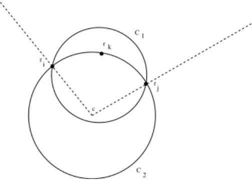
Figure 1 illustrates Property 2.
c C r i 1 C 2 k r j r
Fig. 1. C2is an enclosing circle for the three points ri, rjand rk. However, there
is no point in the intersection between C2 and the concave sector formed by ri,
rj and the center c of C2. So, C2 can be replace by a smaller enclosing circle,
here C1, even if all the points are on the circumference of C2.
Observation 1 Given three colinear points, c,r,r’. If c is on the segment [r, r′],
then c cannot be on the circumference of a circle enclosing r and r′.
Definition 4 (Convex Hull). [16] Given a set P of n ≥ 2 points p1, p2,· · · , pn
on the plane, the convex hull of P, denoted H(P) , is the smallest polygon such that every point in P is either on an edge of H(P) or inside it.
Informally, it is the shape of a rubber-band stretched around p1, p2,· · · , pn.
The convex hull is unique and can be computed with time complexity O(n log n) [16]. When no ambiguity arises, H(P) will be shortly denoted by H and H(P) ∩ P will indicate the set of the positions both on H(P) and P.
From Definition 4, we deduce the following property :
Property 3. Let P be respectively a set of n ≥ 2 points that are not on the same
line and let H(P) be a convex hull. The two following properties are equivalent 1. Any point c, not necessarily in P, is located on H (either on a vertice or an
edge)
2. there is a concave or a straight sector S in {rcr′, rcr′} such that r and r′ are
in P and there exists no point ∈ P ∩ S.
The relationship between the smallest enclosing circle and the convex hull is given by the following property
Property 4. [3] Given a set P of n ≥ 2 points on the plane. We have
SEC(P) ∩ P ⊆ H(P) ∩ P .
The Algorithm Based on the definitions and basic properties introduced above, we are now ready to present a deterministic self-stabilizing algorithm that allows n robots (n odd) to gather in a point, regardless of the initial po-sitions of the robots on the plane. The idea of our algorithm is as follows : It consists in transforming an arbitrary configuration P into one where there is exactly one point pmax∈ M axP. When such a configuration is reached, all the
robots which are not located at pmax move towards pmax avoiding to create
another point q than pmaxsuch that |q| ≥ pmax.
When |M axP| 6= 1, we will distinguish two cases : |M axP| = 2 and |M axP| ≥ 3.
If M axP = {pmax1; pmax2}, then each robot which is not located neither on pmax1nor pmax2 moves towards its closest position ∈ M axP by avoiding to create an adding maximal point. Since the number of robots is odd, we have eventually either |pmax1| > |pmax2| or |pmax1| > |pmax2| and then, |M axP| = 1.
For the case |M axP| ≥ 3, our strategy consists in trying to create a unique maximal point inside SEC. To reach such a configuration, we distinguish three subcases :
1. If there is no robot inside SEC, then all the robots are allowed to move towards the center of SEC.
2. If all the robots inside SEC are located at the center of SEC, then only the robots located in SEC ∩ M axP are allowed to move towards the center of SEC.
3. If some robots inside SEC are not located at the center of SEC, then only the robots inside SEC are allowed to move towards the center of SEC.
The main algorithm is shown in Algorithm 1. In Algorithm 1, we use two subroutines : move to caref ully(p) and choose closest position(p1, p2). The for-mer allows a robot r, located at q, to move towards p only if there is no robot on the segment [q, p] except the robots located on p or the robots located on q. The latter one returns the closest position to r among {p1, p2}. If the distance between r and p1 is equal to the distance between r and p2 then the function
returns p1.
Algorithm 1 Gathering for an odd number of robots, executed by each robot.
P := the set of all the positions;
M axP := the set of all the points p ∈ P such that |p| is maximal; if |M axP| = 1
then pmax:= the unique point in M axP; if I am not on pmax;
thenmove to caref ully(pmax); endif
endif
if |M axP| = 2
then pmax1:= the first point in M axP; pmax2:= the second point in M axP; if I am not neither on pmax1nor pmax2
thenq:= choose closest position(pmax1, pmax2); move to caref ully(q);
endif endif
if |M axP| ≥ 3
thenSEC:= the smallest circle enclosing all the points in P; c:= the center of SEC;
Boundary:= SEC ∩ P; Inside:= P \ Boundary; if Inside6= ∅
then if All the robots ∈ Inside are located at c then if I am in (Boundary ∩ M axP)
thenmove to(c); endif
else if I am in Inside thenmove to(c); endif
endif elsemove to(c); endif
Proof of closure
Lemma 2 (Closure). According to Algorithm 1, if all the robots are located at
the same position p, then all the robots are located at the same position thereafter.
Proof of convergence
Cases |M axP| = 1 and |M axP| = 2.
Lemma 3. Let P be an arbitrary configuration for an odd number of n robots.
According to Algorithm 1, if |M axP| = 1 then all the robots are located at the same position in finite time.
Lemma 4. Let P be an arbitrary configuration for an odd number of n robots.
According to Algorithm 1, if |M axP| = 2 then all the robots are located at the same position in finite time.
Case |M axP| ≥ 3. In this paragraph, we prove that starting from a configuration
where |M axP| ≥ 3, all the robots are located at the same position in finite time. More precisely, we consider the case where there exists at least one robot inside SEC(P(t)) ( refer to Lemma 7) and the case where there is no robot inside SEC(P(t)) ( refer to Lemma 8).
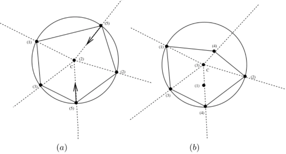
In order to prove Lemma 7, we use Lemmas 5 and 6. In particular, Lem-mas 5 shows that, under specific conditions, the center of SEC(P(t)) is inside SEC(P(t + 1)) even if SEC(P(t)) 6= SEC(P(t + 1)) or the center of SEC(P(t)) is not the center of SEC(P(t + 1)). The proof of Lemma 5 is organized in two parts. In the former one, we consider the case where the center of SEC is also on the convex hull (see Figure 2.c). In the latter one, we consider the case where the center of SEC is not on the convex hull.
Lemma 5. Let P(t) be a configuration such that |M axP| ≥ 3 and there exists
at least one robot inside SEC(P(t)).
According to Algorithm 1, if both conditions are true :
1. some robots ∈ P(t) ∩ SEC(P(t)) move in straight line toward the center c of SEC(t) and,
2. for every p ∈ P(t) ∩ SEC(P(t)) there exists at least one robot in p which does not reach c at time t + 1
then, the center of SEC(P(t)) is inside SEC(P(t + 1)) at time t + 1.
Proof. Let c be the center of SEC(t) at time t. We consider two cases, depending
on whether c is on the convex hull H(P(t)) or not, at time t.
– c is on H(P(t)) at time t. From Property 3, there exists a concave or a straight sector S in {xcy, xcy} such that x and y are in P(t) and there is no point ∈ P(t) ∩ S. However, from Property 2, we know that there do not exist two points x and y in P(t) such that there exists a concave sector S
(5) (1) (3) (5) (2) (2) C (a) (2) (1) C (3) (3) (4) (4) (1) (b)
Fig. 2. The numbers between parenthesis indicate the multiplicity. In Figure a, we have a configuration P(t) where the center c of SEC(P(t)) is inside the convex hull. Figure b, we have configuration P(t + 1) where some robots have moved toward c and c is inside the new convex hull.
in {xcy, xcy} and P(t) ∩ S = ∅. So, there exists only a straight sector S in {xcy, xcy} such that x and y are in P(t) and there is no point ∈ P(t) ∩ S. Consequently, c is on the segment [x, y] at time t. Since the robots move in straight line towards c and since there exist some robots located at x and some robot located at y which do not reach c at time t + 1 then, c is on the segment [r, s] at time t + 1 with r and s ∈ P(t + 1). From Observation 1, we deduce that c is inside SEC(P(t + 1)) at time t + 1.
– c is not on H(P(t)) at time t. In this case, all the points in P(t) are not on the same line otherwise c would have been on H(P(t)). So, from Property 3 we know that there does not exist a concave or a straight sector S in {xcy, xcy} such that x and y are in P(t) and there is no point ∈ P(t) ∩ S. Since the robots move in straight line towards c and since for each point p∈ P(t) there exists at least one robot located on p which does not reach c at time t+1 then, we deduce that there does not exist a concave or a straight sector S in {rcs, rcs} such that r and s are in P(t + 1) and there is no point ∈ P(t + 1) ∩ S (Figures 2.a and 2.b illustrate this fact). So, from Property 3 cis inside H(P(t + 1)) at time t + 1, and from Lemma 4 we deduce that c is inside SEC(P(t + 1)).
Lemma 6. Let P(t) be a configuration such that |M axP| ≥ 3 and there exists
at least one robot inside SEC(P(t)). If any robot r is inside SEC(P(t)) and r is located on the boundary of SEC(P(t + 1)) then |M axP(t + 1)| ≤ 2.
Proof. By contradiction assume that r is inside SEC(P(t)) and r is located
on the boundary of SEC(P(t + 1)) and |M axP(t + 1)| > 2. Let c be the cen-ter of SEC(P(t)) at time t. From assumption, some robots on the boundary
of SEC(P(t)) have moved toward the center of SEC(P(t)). According to Algo-rithm 1, that implies that all the robots inside SEC(P(t)), notably r, are located at the center of SEC(P(t)) at time t. So, c is on the boundary of SEC(P(t+ 1)). From Lemma 5, we deduce that there exists a point p ∈ P(t) ∩ SEC(P(t)) such that all the robots in p have reached c at time t + 1. However, according to Algorithm 1 only the robots located in ∈ M axP(t) ∩ SEC(P(t)) are allowed to move at time t. Therefore, for every point p 6= c we have |c| > |p| at time t + 1. Hence, |M axP(t + 1)| = {c} i.e., |M axP(t + 1)| = 1. A contradiction.
Lemma 7. Let P(t) a configuration such that |M axP| ≥ 3 and there exists at
least one robot inside SEC(P(t)). According to Algorithm 1, all the robots are located at the same position in finite time.
Proof. Assume by contradiction |M axP| ≥ 3 forever. From Lemma 6, we know
that the robots inside SEC(P(t)) are inside SEC(P(t + 1)). So, by induction we deduce that the robots inside SEC(P(t)) are inside SEC(P(ti)) for all ti ≥ t.
From Lemma 1, fairness and because of the fact that each robot r can move to at least a constant distance σr>0 in one step, we know that there exists a
time instant tk where the number of robots at the center of SEC(P(tk)) will be
greater than the number of robots not located at the center of SEC(P(tk)). So,
|M axP| = 1 : contradiction. So, |M axP| ≤ 2 in finite time and from Lemmas 3 and 4 all the robots are located at the same position in finite time.
Lemma 8. Let P(t) be a configuration such that |M axP| ≥ 3 and there exists
no robot inside SEC(P(t)). According to Algorithm 1, all the robots are located at the same position in finite time.
Proof. According to Algorithm 1, all the robots may decide to move toward the
center of SEC. Since each robot r can move to at least a constant distance σr > 0 in one step, if all the robots are always on the boundary of SEC(P)
then, by fairness, the gathering problem is solved in finite time. Otherwise, – either there exists tk> tsuch that |M axP(tk)| ≥ 3 and there exists at least
one robot inside SEC(P(t)) : From Lemma 7, we deduce that all the robots are located at the same position in finite time,
– or there exists tk > tsuch that |M axP(tk)| ≤ 2 : from Lemmas 3 and 4 all
the robots are located at the same position in finite time.
4
Conclusion
Assuming strong multiplicity detection, we provided a complete characterization (necessary and sufficient conditions) to solve the gathering problem. Note that we do not know whether strong multiplicity detection is a necessary condition to solve the gathering problem. In future works, we would like to study the weakest minimal multiplicity detection that solves this problem and under which conditions. Note that the gathering problem seems to be the only positioning problem that can be deterministically and self-stabilizing solved. Indeed, since initially the robots can share the same positions, there exists no deterministic algorithm to scatter them in the plane [8].
References
1. Noa Agmon and David Peleg. Fault-tolerant gathering algorithms for autonomous mobile robots. SIAM J. Comput., 36(1):56–82, 2006.
2. H Ando, Y Oasa, I Suzuki, and M Yamashita. A distributed memoryless point convergence algorithm for mobile robots with limited visibility. IEEE Transaction
on Robotics and Automation, 15(5):818–828, 1999.
3. P Chrystal. On the problem to construct the minimum circle enclosing n given points in a plane. In the Edinburgh Mathematical Society, Third Meeting, page 30, 1885.
4. M Cieliebak, P Flocchini, G Prencipe, and N Santoro. Solving the robots gath-ering problem. In Proceedings of the 30th International Colloquium on Automata,
Languages and Programming (ICALP 2003), pages 1181–1196, 2003.
5. Mark Cieliebak. Gathering non-oblivious mobile robots. In LATIN, pages 577–588, 2004.
6. X Defago and A Konagaya. Circle formation for oblivious anonymous mobile robots with no common sense of orientation. In 2nd ACM International Annual
Workshop on Principles of Mobile Computing (POMC 2002), pages 97–104, 2002.
7. Xavier D´efago, Maria Gradinariu, St´ephane Messika, and Philippe Raipin Parv´edy. Fault-tolerant and self-stabilizing mobile robots gathering. In DISC, pages 46–60, 2006.
8. Yoann Dieudon´e and Franck Petit. Scatter of robots. Parallel Processing Letters, 19(1):175–184, 2009.
9. S. Dolev. Self-Stabilization. The MIT Press, 2000.
10. Paola Flocchini, David Ilcinkas, Andrzej Pelc, and Nicola Santoro. Remembering without memory: Tree exploration by asynchronous oblivious robots. In SIROCCO, pages 33–47, 2008.
11. Paola Flocchini, Evangelos Kranakis, Danny Krizanc, Nicola Santoro, and Cindy Sawchuk. Multiple mobile agent rendezvous in a ring. In LATIN 2004: Theoretical
Informatics, 6th Latin American Symposium, volume 2976 of Lecture Notes in Computer Science, pages 599–608. Springer, 2004.
12. Paola Flocchini, Giuseppe Prencipe, Nicola Santoro, and Peter Widmayer. Gath-ering of asynchronous robots with limited visibility. Theor. Comput. Sci., 337(1-3):147–168, 2005.
13. Ralf Klasing, Euripides Markou, and Andrzej Pelc. Gathering asynchronous obliv-ious mobile robots in a ring. Theor. Comput. Sci., 390(1):27–39, 2008.
14. G Prencipe. Corda: Distributed coordination of a set of autonomous mobile robots. In Proceedings of the Fourth European Research Seminar on Advances in
Dis-tributed Systems (ERSADS 2001), pages 185–190, 2001.
15. Giuseppe Prencipe. Impossibility of gathering by a set of autonomous mobile robots. Theor. Comput. Sci., 384(2-3):222–231, 2007.
16. Franco P. Preparata and S. J. Hong. Convex hulls of finite sets of poin ts in two and three dimensions. Commun. ACM, 20(2):87–93, 1977.
17. Samia Souissi, Xavier D´efago, and Masafumi Yamashita. Using eventually consis-tent compasses to gather memory-less mobile robots with limited visibility. ACM
Trans. Auton. Adapt. Syst., 4(1):1–27, 2009.
18. I Suzuki and M Yamashita. Agreement on a common x-y coordinate system by a group of mobile robots. Intelligent Robots: Sensing, Modeling and Planning, pages 305–321, 1996.
19. I Suzuki and M Yamashita. Distributed anonymous mobile robots - formation of geometric patterns. SIAM Journal of Computing, 28(4):1347–1363, 1999.
Annexes
Lemma 2. According to Algorithm 1, if all the robots are located at the same position p, all the robots are located at the same position thereafter.
Proof. If all the robots are located at the same position p, then |M axP| = 1 and all the robots are located at the unique position p ∈ M axP. According to Algorithm 1, in the case |M axP| = 1 the robots located on p remains idle. So, all the robots are located at the same position forever.
Lemma 3. Let P be an arbitrary configuration for an odd number of n robots. According to Algorithm 1, if |M axP| = 1 then all the robots are located at the same position in finite time.
Proof. Let pmax be the unique point in M axP(t). According to Algorithm 1,
the robots located on pmaxduring step (t, t+1) remains idle. Moreover, according
to Algorithm 1 and Function move to caref ully(), if two robots ri and rj are
not at the same point at time t, i.e., pi(t) 6= pj(t) then pi(t + 1) 6= pj(t + 1) at
time t + 1 unless they have reached pmax. Hence, pmaxremains the unique point
in M axP(tk), for all tk ≥ t. So, according to Algorithm 1 and by fairness, we
deduce that |pmax| = n in finite time.
Lemma 4. Let P be an arbitrary configuration for an odd number of n robots. According to Algorithm 1, if |M axP| = 2 then all the robots are located at the same position in finite time.
Proof. The proof is organized as follows : First, we prove that there exists tk ≥ t
such that |M axP(tk)| 6= 2. Then, we prove that there does not exist any time
tk≥ t such that |M axP(tk)| ≥ 3. Finally, we deduce that Lemma 3 holds.
1. Assume by contradiction that there does not exist any time tk ≥ t such
that |M axP(tk)| 6= 2. Consequently, for every tk ≥ t, |M axP(tk)| = 2. Let
pmax1 and pmax2 be the two points in M axP(t) at time t. According to
Algorithm 1, the robots located either on pmax1 or on pmax2 during step
(t, t + 1) remains idle. Moreover, according to Algorithm 1 and Function move to caref ully(), if two robots ri and rj are not at the same point at
time t, i.e., pi(t) 6= pj(t) then pi(t + 1) 6= pj(t + 1) at time t + 1 unless
either ri and rj have reached pmax1 or ri and rj have reached pmax2. So,
by induction we deduce that pmax1 and pmax2 remains the only positions in M axP(tk) for every tk ≥ t. By fairness, we deduce that, all the robots
are either at pmax1 or at pmax2 in finite time. However, since the number of
robots is odd then, we have either |pmax1| > |pmax2| or |pmax1| < |pmax2|.
Hence, |M axP(tk)| = 1 : Contradiction.
2. Assume by contradiction that there exists tk≥ t such that |M axP(tk)| ≥ 3.
Without lost of generality, we assume that tk is the first time for which
tk and |M axP(tk)| = 1 : Indeed from Lemma 2 and the proof of Lemma 3,
once there exist a unique point pmax then, it remains the unique point in
M axP forever and that would be a contradiction. Hence, |M axP(tk− 1)| = 2.
Let pmax1 and pmax2 be the two points in M axP(tk − 1) at time tk− 1.
According to Algorithm 1, the robots located either on pmax1 or on pmax2
during step (t, t + 1) remains idle. Besides, according to Algorithm 1 and Function move to caref ully(), if two robots ri and rj are not at the same
point at time tk− 1, i.e., pi(tk− 1) 6= pj(tk− 1) then pi(k) 6= pj(k) at time tk
unless either ri and rj have reached pmax1 or ri and rj have reached pmax2.
So, |M axP(tk)| ≤ 2 at time tk. A contradiction.
From above, we deduce that if |M axP(t)| = 2 at time t then, according to Algorithm 1 there exists tk, tk > tsuch that |M axP(tk)| = 1. So, from Lemma 3,