Cell phone location data for travel behavior analysis

(1)

Cell Phone Location Data for Travel Behavior

Analysis

by

Lauren P. Alexander

B.S., University of Texas at Austin (2009)

ARCHNE8

MASSACHUSETTS INSTITUTE

OF TECHNOLOLGY

JUL 02 2015

LIBRARIES

Submitted to the Department of Civil and Environmental Engineering

in partial fulfillment of the requirements for the degree of

Master of Science in Transportation

at the

MASSACHUSETTS INSTITUTE OF TECHNOLOGY

June 2015

@

Massachusetts Institute of Technology 2015. All rights reserved.

Author.

_{A u h}

_{r ..}

_...

...

....

Signature redacted

-Department of Civil and' Environmental Engineering

May 21, 2015

Signature redacted

C ertified by

...

Marta C. Gonzailez

Associate Professor of Civil and Environmental Engineering Thesis Supervisor

Accepted by...Signature

redacted

Heidi M. N pf

Donald and Martha Harleman Professor of Civil and Environmental Engineer ng Chair, Departmental Committee for Graduate Students

(2)

(3)

Cell Phone Location Data for Travel Behavior Analysis

by

Lauren P. Alexander

Submitted to the Department of Civil and Environmental Engineering on May 21, 2015, in partial fulfillment of the

requirements for the degree of Master of Science in Transportation

Abstract

Mobile phone technology generates vast amounts of data at low costs all over the world. This rich data provides digital traces when and where individuals travel, im-proving our ability to understand, model, and predict human mobility. Especially in this era of rapid urbanization, mobile phone data presents exciting new opportunities to plan transportation infrastructure and services that meet the mobility needs and challenges associated with increasing travel demand. But to realize these benefits, methods must be developed to utilize and integrate this data into existing urban and transportation modeling frameworks.

In this thesis, we draw on techniques from the transportation engineering and urban computing communities to estimate travel demand and infrastructure usage. The methods we present utilize call detail records (CDRs) from mobile phones in conjunction with geospatial data, census records, and surveys, to generate represen-tative origin-destination matrices, route trips through road networks, and evaluate traffic congestion. Moreover, we implement these algorithms in a flexible, modular, and computationally efficient software system. This platform provides an end-to-end solution that integrates raw, massive data to generate estimates of travel demand and infrastructure performance in any city, and produces interactive visualizations to effectively communicate these results. Finally, we demonstrate an application of these data and methods to evaluate the impact of ride-sharing on urban traffic.

Using these approaches, we generate travel demand estimates analogous to many of the outputs of conventional travel demand models, demonstrating the potential of mobile phone data as a low cost option for transportation planning. We hope this work will serve as unified and comprehensive guide to integrating new big data resources into transportation modeling practices.

Thesis Supervisor: Marta C. Gonzilez

(4)

(5)

Acknowledgments

First and foremost, I want to thank my advisor, Marta, for her support and contagious enthusiasm. She introduced me to a field of interdisciplinary research, which I find fascinating and meaningful. I truly appreciate the flexibility she has afforded me to explore this new world, while being there to patiently guide me along the way.

To all of my HuMNet friends, thank you for the countless conversations and laughs. Being surrounded every day by such an intelligent, passionate, and fun(ny) group of people is something I will never forget and can only hope to find again. And to my other officemates, classmates, and professors, thank you for helping to make my time at MIT enjoyable and enriching.

To my SDG colleagues, thank you for sparking my interest in transportation. Beginning with the red bus/blue bus lesson on day 1, you taught me, inspired me, and supported me on my path to MIT. To my Bridj colleagues, thank you for the opportunity to apply theory in practice this summer to move real people from point

A to B; it was a truly rewarding experience that cemented my desire to work at the

intersection of transportation and data science.

To my sisters, thank you for always being there for me, and especially for your silliness. To Drew, thank you for your endless support despite taking the brunt of my stress these past two years. And to all of my friends and family, I would be lost without you in my life. Despite distance and busy schedules, know that you are always on my mind. And from the bottom of my heart, thank you.

But most of all, thank you to my parents for the abundance of encouragement, advice, and unconditional love. I am lucky to have two amazing role models who continue to inspire me personally and professionally. You've both shown me that working hard and enjoying what you do can go hand-in-hand, and I will forever strive for this goal.

(6)

(7)

List of Figures

1-1 Schedule-based, tour-based, and trip-based travel demand modeling frameworks. Trip-based models represent unlinked trips, tour-based models chains these trips into tours, and schedule-based models sched-ule these tours. Source: http://ocw.mit

.edu/courses/civil-and-environmental-engineering/1-201j -transportation-systems-analysis-demand-and-economics-fall-2008/lecture-notes/MIT_201JF08_

lecO5.pdf... ... 21

2-1 Extracting stay and pass-by areas from the phone data for an anony-mous user in the 2-month period . . . . 32

2-2 (a) Probability distribution of Census tract expansion factors. (b) The-matic map showing the spatial distribution of Census tract expansion factors. . . . . 36 2-3 Frequency of weekday observations per user. (a) Probability

distribu-tion of total weekday trips per user. (b) Probability distribudistribu-tion of total weekday days per user. (c) Probability distribution of average weekday trips per user. . . . . 38

2-4 (a) CDR residents vs. 2010 Census population by town before and after population expansion. (b) CDR vs. Census Transportation Planning Products (CTPP) 185] workers by town before and after population expansion. . . . . 39

(12)

2-5 Distribution of average weekday hourly departure time from CDR data, 1991 Boston Household Travel Survey (BHTS)

117],

the 2010/2011 Massachusetts Travel Survey (MHTS) [61], and 2009 National House-hold Travel Survey (NHTS) [84] for (a) Home-based Work Trips, (b) Home-based Other Trips, (c) Non-home Based Trips, and (d) All Trips. 41

2-6 (a) Probability density distributions of aggregation area size by des-ignated areas (tract or towns) and variable buffers. (b) Correlation between HW CDR and 2006-2010 CTPP [85] flows corresponding to the aggregation levels in (a). . . . . 43

2-7 (a) Intra-town and inter-town pair daily HW CDR flows and 2006-2010 CTPP 185] flows. (b) Spatial distribution of daily inter-town HW CDR flows (>1,000). (c) Spatial distribution of daily inter-town HW

2006-2010 CTPP [85] flows (>1,000). . . . . 44

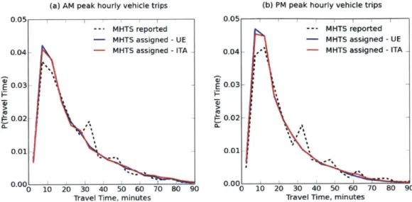
3-1 Travel time (in minutes) distribution of assigned CDR and MHTS trips,

as well as average travel time as reported in the MHTS survey for (a) AM and (b) PM peak hourly vehicle trips. . . . . 54

3-2 2D histogram of community-pair MHTS and CDR vehicle trips in the

(a) morning (AM, 6a-9a) and (b) evening (PM, 3p-7p) peak periods. . 56 3-3 Distribution of average tract-pair travel time (in minutes) of assigned

CDR and MHTS trips for (a) AM and (b) PM peak hourly vehicle trips. 58 3-4 Distribution of road segment volumes of assigned CDR and MHTS

trips for (a) AM and (b) PM peak hourly vehicle trips. . . . . 58 3-5 (a) Road Segment Volume and (b) Volume over Capacity ratio for

MHTS and CDR hourly vehicle trips in the AM and PM peaks. . . . 59

4-1 A flowchart of the system architecture. . . . . 65

4-2 Our efficient implementation of the incremental traffic assignment (ITA) model. A sample OD matrix is divided into two increments and then split into two independent batches each. . . . . 73

(13)

4-3 Correlations between OD matrices produced by our system and those derived from travel surveys at the largest spatial aggregation of the two models. In Boston, this is town-to-town, in San Francisco, MTC superdistrict-to-super district, in Rio, census superdistrict-to-superdistrict, and in Lisbon, freguesia-to-freguesia. The larger of these area units (e.g. towns in Boston), the better our correlations, while correlations at the smallest aggregates(e.g. freguesias in Portugal), correlations are low er. . . . . 75

4-4 Distributions of travel volume assigned to a road and the volume-over-capacity (V/C) ratio for the five cities. The values presented in the legend refers to the fraction of road segments with V/C > 1. . . . . 76

4-5 A graphical representation of the bipartite network of roads and sources (census tracts), with edge sizes mapping the number of users using the connected road in their individual routes. . . . . 77

4-6 Two screen images from the visualization platform. (a) The trip pro-ducing (red) and trip attracting (blue) census tracts using Cambridge St., crossing the Charles River in Boston. (b) Roads used by trips generated at the census tract including MIT. . . . . 78

5-1 (a) Probability distribution of community areas in miles2 _{and (b)}

Spa-tial distribution of community areas, with area increasing from light to dark shades of green. . . . . 90

(14)

5-2 Percent change in total vehicles 6V relative to the ratio of driver and non-driver adoption rates ad/ao. 6V is proportional to the difference between driver and non-driver rideshare trip shares (ad * d - a, * o), as

described by the model: 6V = -0.5922 * (ad * d - ao * o) + 0.0175. In

other words, there is a reduction in vehicles (6V < 0) when the number

of ridesharers diverted from drivers is greater than those diverted from non-drivers (ad * d

>

ao * o). Given the average mode shares of drivers

(d = 70.0%) and non-drivers (fo = 21.5%) in Boston, this relationship

results in an overall reduction in vehicles for ao < 3.2 6*ad, as illustrated

by the data and model. . . . . 96 5-3 (a) Percent change in total vehicles 6V relative to the ratio of driver

ad and non-driver adoption rates ao as estimated by the model 6V =

-0.5922 * (d * ad - o * a0) + 0.0175. (b) Percent change in total vehicles

6V relative to the ratio of driver ad and non-driver ao adoption rates

from the data. (c) Percentage of ridesharers that diverted from non-driving modes (o * ao)/(d * ad + o * ao) relative to the ratio of driver

ad and non-driver ao adoption rates from the data. The black line on

each plot is described by ao = 3.26 * ad, approximately representing

(15)

List of Tables

2.1 _{Average weekday trip shares by purpose and period from CDR data,}

1991 Boston Household Travel Survey (BHTS) [171, the 2010/2011

Massachusetts Travel Survey (MHTS) [61] and the 2009 National House-hold Travel Survey (NHTS) [84] .. . . . . 40 2.2 Average daily trips by purpose and period from CDR data and the

2010/2011 Massachusetts Travel Survey (MHTS) [61], as well as the correlation coefficients of CDR and MHTS tract-pair and town-pair trips. 42

2.3 Comparison of average weekday HW CDR and 2006-2010 CTPP [851

flows... 42

3.1 Average daily vehicle trips by period from CDR data and the 2010/2011 Massachusetts Travel Survey (MHTS) [61], as well as the correlation coefficients of CDR and MHTS community-pair trips. . . . . 55 3.2 Inter-tract vehicle trips, average travel time, and average distance for

the AM and PM peak hours from CDR data and the 2010/2011 Mas-sachusetts Travel Survey (MHTS) 161]. . . . . 57

4.1 A comparison of the extent of the data involved in the analysis of the

(16)

4.2 Trip tables estimates. Where possible, our results are compared to estimates made using travel surveys. For each city, we report the num-ber of person trips in millions for a given purpose or time. Trip pur-poses include: home-based word (HBW), home-based other (HBO), and non-home-based (NHB). Trip periods include: 7am-10am (AM), 10am-4pm(MD), 4pm-7pm (PM), and the rest of the day (RD). We note that the exact boundaries of the surveys do not exactly coincide with those used in our estimation so direct comparisons are not ex-act. No comparisons could be found for Porto. *Note that the Lisbon Survey only contains estimates of vehicle trips in millions. . . . . 74

5.1 Percent change in vehicles, vehicle miles traveled (VMT), vehicle hours traveled (VHT), and congested travel time (TT) relative to drive-alone/taxi and other non-auto adoption rates ad, a, = 0. Results are

(17)

Chapter 1 Introduction

1.1 Overview and motivation

According the United Nations Population Fund (UNFPA), 2008 marked the first year in which the majority of the world's population lived in cities. Rapid urbanization places enormous strain on already burdened transportation infrastructure critical to providing residents with access to places, people, and goods. Delays and poor levels of service resulting from such congestion waste time and money and exacerbate harmful vehicle emissions.

Effectively moving people and goods-the fundamental task of transportation plan-ners, modelers, and engineers-is increasingly challenging in this era of rapid popu-lation growth in cities. Meanwhile, transportation services and infrastructure effect economic growth and quality of life within cities. Given the direct and varied im-pacts it has on society, the transportation industry attracts planners, engineers, and economists to address these complex challenges.

Interdisciplinary approaches are key to understanding and modeling human mobil-ity patterns and future mobilmobil-ity needs. The economists' principles of supply, demand, and pricing, along with the planners' concepts of transportation system dynamics, un-derpin much of the framework for modeling human mobility. Combining broad and varied expertise, cities can adopt strategies to plan more efficient, sustainable, and equitable transportation systems.

(18)

Travel demand models are essential for managing existing transportation systems and planning for future development. Demand estimates output from such models are relied upon for transportation plans, environmental impact studies, and infrastructure investment and prioritization decisions [11]. Travel demand models widely-used in industry fall into two main categories: the traditional four-step or trip-based models, and the newer activity-based or schedule-based models.

But despite the sophistication of these models, they require quality input data for development, calibration, and validation. Accordingly, a large amount of time and money are spent on data collection. Data demands include detailed data on transportation networks, capacities, and levels of service, as well as behavioral data collected from surveys. In addition to sociodemographic information, household travel surveys provide travel-activity diaries detailing specific trips and travel characteristics of the respondent. Because they are expensive and intrusive, such surveys typically describe just one recent day, limiting their ability to capture irregular and/or leisure activities.

In contrast to survey data, ubiquitous mobile computing, namely the pervasive use of cellular phones, has generated a wealth of data that can be analyzed to under-stand and improve urban infrastructure systems. The penetration of these devices is astounding with six billion mobile phones nearly tripling the number of internet users. Penetration rates of over 100% are routinely found in the developed word, e.g. 104% in the United States and 128% in Europe1 and rates are of over 85%2 are observed developing contexts. These devices and the applications that run on them passively record social, mobility, and a variety of other behaviors of their users with extremely high spatial and temporal resolution.

However, before the benefits of this massive, passive data can be realized within the transportation domain, methods must be developed and assessed with respect to their applicability and limitations. In particular, mobile phone data has the potential 1_{GSMA European Mobile Industry Observatory 2011 http: //www} _._gsma.

com/publicpolicy/wp-content/uploads/2012/04/emofullwebfinal.pdf

2_ITU.

(2013) ICT Facts and Figures http: //www. itu. int/en/ITU-D/Statistics/Documents/

(19)

to complement or substitute for household travel surveys. However, despite the fact that it can be gathered more frequently and economically, mobile phone data lacks information about a respondent (e.g. age or income) or his/her trip (e.g. purpose or mode) [70, 81, 44]. Furthermore, mobile phone data contains traces of a user at approximated locations when his/her phone communicates with a cell phone tower, providing an inexact and incomplete picture of daily trip-making. Accordingly, much research has focused on developing methods to extract meaningful information about human mobility from mobile phone traces.

Adding to the existing body of work using mobile phone data, we present method-ology to go from raw mobile phone data to road usage, analogous to the trip genera-tion, trip distribugenera-tion, mode choice, and traffic assignments procedures of traditional travel demand models. By paralleling the framework commonly used by transporta-tion planners and modelers, we are able to compare and contrast these methods and results with traditional survey data and models. Moreover, we present a flexible, modular, and computationally efficient software system to integrate these algorithms and visualize results in any city for which mobile phone data is available. Lastly, we present an application that utilizes all of these methods to evaluate the impact of ridesharing on urban traffic.

The gamut of travel demand estimation using big data resources is presented through the methods, validation, implementation, and applications described in this thesis. Demonstrating the validity of mobile phone data as an end-to-end solution for travel demand estimation will hopefully support the incorporation of new big data resources into transportation demand modeling approaches.

1.2 Literature review

Researchers across different domains approach travel demand modeling in different ways. Here, we present an overview of bodies of work in two communities, in particu-lar: transportation engineering and urban computing. The transportation engineering community typically uses models to derive demand and behavior based on

(20)

nomic, land use, and transportation characteristics. The urban computing community brings together statistical models, data mining, and machine learning techniques to extract mobility patterns from large amounts of data. As automatically collected data is becoming more widespread, the boundary between these communities is di-minishing.

1.2.1 Transportation engineering

Travel demand models are widely used for transportation policy, planning, and en-gineering applications in order to estimate infrastructure capacity requirements, fi-nancial and social viability, and environmental impacts of proposed transportation projects. The fundamental task of these models is to adequately model the travel decision process, a problem simplified by aggregating decisions and decision-makers in space (e.g. dividing a study area into zones) and time (e.g. discrete time periods). Travel demand models were first developed in the US in response to post-war de-velopment and economic growth, with the first comprehensive application being the Chicago Area Transportation Study in the 1950s. This study implemented a four-step model, modeling estimation procedures in four sequential four-steps: trip generation, trip distribution, mode choice, and trip assignment. Federal legislation introduced in the 1960s requiring urban transportation planning institutionalized the four-step model. In the 1970s additional legislation called for improved models, with particu-lar emphasis on multimodal and environmental planning, leading to the development and integration of more sophisticated demand and assignment methods into four-step models. Growing recognition of the limitations of the four-step modeling approach in the late 1970s and 1980s led to Travel Model Improvement Program3_{, which has}

worked towards advancing modeling capabilities and supporting transportation pro-fessionals since the early 1990s. Efforts in the last few decades can be characterized as improving of-the-practice conventional models while further developing state-of-the-art methodologies [57].

Approaches to modeling travel demand fall into three main categories-trip-based,

(21)

Schedule

_Tours

_Trips

Space space Space

H _H H W

w

S H-S H S H H ""0 S D H: D H D H H-D H

Ti1me rTome ime

H: Home W: Work S: Shop D: Dinner out

Figure 1-1: Schedule-based, tour-based, and trip-based travel demand modeling frameworks. Trip-based models represent unlinked trips, tour-based models chains these trips into tours, and schedule-based models schedule these tours. Source:

http://ocw.mit.edu/courses/civil-and-environmental-engineering/1-201j- transportation-systems-analysis-demand-and-economics-fall-2008/lecture-notes/MIT1_201JF08_lecO5.pdf

tour-based, and schedule-based, as summarized in Figure 1-1. Trip-based models represent unlinked trips, tour-based models chains these trips into tours, and schedule-based models schedule these tours. The four-step model is an example of a trip-schedule-based approach, while newer activity-based models use the schedule-based approach.

Four-step models-still the most widely used model in practice-are developed, up-dated, and applied by many metropolitan planning organizations (MPOs) and plan-ning agencies across the US and abroad. In contrast to microscopic agent-based models, this framework aggregates travelers and trips at the level of traffic analysis zones (TAZs) rather than simulating travel behavior of individuals. Each of the four steps are described in more detail below:

1. Trip generation: This step determines trip origins and destinations based on

the distribution of households, employment, and land use. More specifically, trip productions are estimated based on household characteristics such as size, income,

(22)

car ownership, density, and accessibility. Similarly, trip attractions are estimated using land use, employment by sector, and accessibility data. The models in this step typically use regression [37, 48, 56, 62], cross classification [68], and growth factor analysis.

2. Trip distribution: This step estimates the distribution of trips as a function

of the generalized cost of travel between origins and destinations. Trip distribution uses the origins and destinations estimated in the first step as marginal totals from which to estimate the elements of a trip matrix. Various aggregate models of trip distribution have been proposed [63, 82, 90, 91, 92, 951. Among all these efforts, the gravity model, which assumes that the number of movements between an OD pair decays with their distance or cost, is the most widely used [95, 28, 33]. When an empirical OD matrix is available from survey data, for example, a method called iterative proportional fitting (IPF) method can be used [75]. This procedure adjusts matrix values from the input (or seed) matrix, in order to match the input row and column totals (or marginals).

3. Mode choice: This step computes the share of origin-destination (OD) trips

that use each available transportation mode. This step is dominated by discrete choice models [16, 15, 59, 27], which model choices between discrete alternatives using an economic utility-maximization framework. Here, a decision maker selects the alternative (in this case mode) with the highest utility among all the alternatives in the choice set. The utility of an alternative is modeled as a function of the characteristics of traveler (i.e. socioeconomic characteristics) and the characteristics of each travel mode (i.e. levels of service such as time and cost). Logit models, which can take on a nesting structure to model hierarchy in the decision-making process, are most commonly used to compute mode shares.

4. Trip assignment: This step allocates origin-destination trips of a given mode to a particular path or route. Route choice can be modeled as a deterministic choice (i.e. shortest path or minimum generalized cost), or a stochastic choice (i.e. discrete choice using a logit model). Moreover, modeling approaches can use non-equilibrium, heuristic assignment methods (i.e. all-or-nothing or incremental traffic assignment)

(23)

or equilibrium methods (i.e. user optimal or system optimal). Lastly, traffic as-signment can be dynamic (DTA) which uses an equilibrium approach at fine-grain temporal intervals (i.e. real-time or pseudo real-time)

158],

or static assignment, which assumes fixed-demand typically at the interval of an hour. All of these assignment methods incorporate the relationship between volume, capacity, and travel time using volume-delay functions such as the Bureau of Public Roads (BPR), conical congestion function, and Akcelik flow delay function.

As we use iterative traffic assignment (ITA) due its computational advantages in subsequent chapters, we present more detail on the limitations of this traffic assign-ment heuristic. ITA is a static, non-equilibrium method which assigns batches (e.g. 40%, 30%, 20%, 10%) of trips serially and updates costs between increments, an im-provement over all-or-nothing assignment. However, it does not represent the optimal traffic assignment outcome. The smaller the increments, the closer this method is to user equilibrium algorithms, and the closer the solution is to the Wardrop principles

[88], or Nash Equilibria, where in the final traffic conditions, no driver has an incentive

to change their route as all driver paths minimize their total travel time. Despite its wide-use, the four-step model has several limitations, including:

1. demand is modeled for trips rather than activities, which governs trip-making

in reality; and

2. trips are the unit of analysis, therefore interdependence of trips cannot be cap-tured; and

3. aggregating trips by discrete spatial, temporal, and demographic characteristics

introduces errors; and

4. the sequential nature of the four-step procedure does not enable interdependence of these choices.

These limitations led to the development of activity-based models, which use a schedule-based approach illustrated in Figure 1-1. Under this method, travel demand is derived from demand for activities rather than trips themselves, sequences of trips

(24)

are modeled as interdependent tours, and activity and travel scheduling constraints impact travel decisions [7, 18, 69, 83]. Activity-based models replace the trip

genera-tion and distribugenera-tion of four-step models, instead modeling the number, purpose, and sequence of tours. First, the model predicts activity patterns, including a primary tour type and the number and purpose of secondary tours. Next, the model estimates the timing, destination, and mode of primary tours, followed by that of the secondary tours. Despite its benefits, activity-based models have much larger choice sets and are therefore computationally burdensome, and are still unable to completely represent schedules and constraints.

Both four-step and activity-based models rely heavily on survey data for develop-ment, calibration, validation. These models combine meticulous methods of statistical sampling in local [31, 76] and national household travel surveys [81, 70] to process and infer trip information between areas of a city. Travel surveys are typically adminis-tered by state or regional planning organizations and are integrated with public data such as census tracts and the demographic characteristics of their residents, made available by city, state, and federal agencies. While the surveys that provide the empirical foundation for these models offer a combination of highly detailed travel logs for carefully selected representative population samples, they are expensive to administer and participate in. As a result, the time between surveys range from 5 to

10 years in even the most developed cities.

The estimates these surveys and models produce are critically important for un-derstanding the use of transportation infrastructure and planning for its future[86,

79, 54, 51, 43, 42, 41, 52, 25, 13j. As data becomes better and more widely available,

models continue to improve, and computational resources increase, they are increas-ingly useful and accurate tools for transportation planning applications. Modeling methods are increasingly moving from aggregate to disaggregate models and from static to dynamic procedures, as with more detailed agent-based, microsimulation models. Such trends also support more detailed representation of behavior, captur-ing more heterogeneous populations and preferences, and complex, interdependent trip-making.

(25)

Given the complexity of travel demand estimation procedures, several widely-used commercial software packages exist to implement these models. The vast majority of travel demand models used in practice are implemented in TransCAD, Cube, or Emme. These three software platforms consist of standard GIS capabilities as well as built in functions supporting travel demand forecasting, including four-step and activity-based modeling procedures. These proprietary software platforms are up-dated to incorporate state-of-the-art methods and use menu-based graphical user interfaces (GUIs) for ease of use, but are expensive and are considered by some to be

black boxes, with their inner workings unknown to most users.

1.2.2 Urban computing

The interdisciplinary field of urban computing has emerged in recent years, developing computational methods focused on supporting livable, efficient, and sustainable cities for generations to come [47]. Central to this research are estimates of where, when, and how people move within a city and use its facilities. Here, we focus on methods of urban computing as they relate to human mobility patterns.

Given the heterogeneity of urban populations, as well as the immense number of activities and spatial and temporal options in which to perform to these activities, mobility estimates have proved difficult to attain. Moreover, stochasticity is present not only in individuals' choices of locations, times, and activities, but also their travel modes, routes, and trip sequences used to perform these activities. Despite this complexity, however, researchers have found that human mobility can in fact be characterized by regularity and preferential attachment, enabling the development of models to predict mobility patterns [78, 77, 38, 40, 20].

At the same time, technological advances such as increased storage capacity and cloud computing has made it possible to capture petabytes of data from individuals worldwide, from internet usage, credit card transactions, GPS-equipped vehicles, and transit smart cards. These data streams produce massive amounts of time-stamped location data saved in real-time [30, 21, 34]. However, these data pale in comparison to that produced by mobile phones around the globe. Given the frequency of use and

(26)

penetration of these ubiquitous devices, they serve as effective sensors of our daily movement.

Mobile phones provide digital footprints of our whereabouts anytime we send a text, make a phone call, or browse the web. Moreover, even when we aren't interacting with our phones, they periodically communicate with cellular network access points and towers. And given the ability to store such data at decreasing costs year after year, such data is increasingly being collected by mobile phone providers. This rich source of data presents new opportunities to understand, infer, and predict human behavior

135].

In developing countries, which often lack reliable data resources such as local and national surveys, mobile phones are a particularly promising source of mobility information. Especially in these contexts, mobility data from mobile phones could be crucial for modeling epidemic spreading, disaster and emergency evacuation response, and effective resource allocation.

Data generated by the pervasive use of cellular phones has offered insights into ab-stract characteristics of human mobility patterns. Recent work has found that individ-uals are predictable, unique, and slow to explore new places [38, 20, 32, 78, 77, 24, 23J. The availability of similar data nearly anywhere in the world has facilitated compar-ative studies that show many of these properties hold across the globe despite differ-ences in culture, socioeconomic variables, and geography. The benefits of this data have been realized in various contexts such as daily mobility motifs [73, 74], disease spreading [12, 89] and population movement [531. While these works have laid an important foundation, there still is a need to integrate these data into transportation planning frameworks.

Individual survey tracking and stay extraction [81, OD-estimation and validation [22, 60, 87, 46], traffic speed estimation

19,

94], and activity modeling [64, 67] have all been explored using new massive, passively collected data. However, these studies generally present alternatives for only a few steps in traditional four-step or activ-ity based models for estimating travel demand or fail to compare outputs to travel demand estimates from other sources. Moreover, many methods offered to date lack portability from one city to many with minimal additional data collection or

(27)

calibra-tion required.

1.3 Outline

The remaining chapters of this thesis present methods and applications using mobile phone data for travel demand estimation.

Chapter 2 presents methods, results, and validation of estimates of origin-destination trips by purpose and time of day using mobile phone data. The results of this chap-ter are analogous to outputs of the first two steps of four-step travel demand models: trip generation and trip distribution. Chapter 3 follows with methods, results, and validation of estimates of vehicle trips and road usage, analogous to the last two steps of four-step travel demand models: mode choice and traffic assignment. The methods described in both chapters are applied to mobile phone data in Boston, demonstrat-ing the applicability and validity of these methods compared with local and national survey data.

Chapter 4 presents an overview of a portable, efficient software platform built to implement the methods presented in Chapter 2 and 3. This system enables re-searchers to import mobile phone data sets to produce trip matrices and road usage in any city. Moreover, the platform visualizes these outputs to effectively communi-cate mobility patterns to planners, stakeholders, and decision-makers. The platform is an alternative to expensive proprietary transportation software packages and built specifically to handle massive mobile phone data sets and additional, open-source data. Results are presented for five cities in the US, Latin America, and Europe, demonstrating the flexibility and extensibility of the platform.

Chapter 5 presents an application of the methods developed in previous chapters. Here, we evaluate the impact of ridesharing on urban traffic. Assuming hypothetical adoption rates of ridesharing, we estimate the number of rideshare vehicles and change in total, network-wide vehicles. Here, we use travel demand estimated in Chapter 2, and modify methods in Chapter 3 to measure the impact of rideshare service on urban congestion in Boston.

(28)

Each chapter begins with an introduction, follows with descriptions of data and methods, and concludes with a discussion of results and conclusions. Although each chapter can stand-alone, they reference and build upon ideas and methods covered in previous chapters. Accordingly, each chapter provides context useful for understand-ing subsequent methods and applications. Finally, we summarize the over-archunderstand-ing results, limitations, and applications of this work in Chapter 6. Appendix A provides pseudo-code describing the algorithms presented in Chapters 2 and 3 as they are implemented in Chapter 4.

(29)

Chapter 2 Inferring origin-destination trips by

purpose and time of day

2.1 Introduction

The ubiquity of cell phones, along with rapid advancement in mobile technology, has made them increasingly effective sensors of our daily whereabouts [49]. Call detail records (CDRs) from mobile phones contain time-stamped coordinates of anonymized customers, thereby providing rich spatiotemporal information about human mobility patterns. Since CDRs are automatically collected by cell phone carriers for billing purposes, this data can be gathered more frequently and economically than travel survey data collected once (or twice) a decade for transportation planning purposes. Additionally, mobile phone data offers digital footprints at a scale and resolution that may not be captured by surveys that typically record one day of travel diaries per household.

Despite these advantages, mobile phone data lacks information typically avail-able from travel surveys about a respondent (e.g. age or income) or his/her trip (e.g. purpose or mode)

170,

81, 44]. Furthermore, CDRs contain traces of a user at

approximated locations when his/her phone communicates with a cell phone tower, providing an inexact and incomplete picture of daily trip-making. Accordingly, much research has focused on developing methods to extract meaningful information about

(30)

human mobility from mobile phone traces as well as understanding its limitations. It has been demonstrated that CDR data can be used to infer origin-destination

(OD) trips using microsimulation and limited traffic count data [46]. At the level

of the individual, daily trip chains

/trajectories

constructed from mobile phone data are consistent with household surveys [47, 73]. Further, road usage inferred from the CDR data has been validated against GPS speed data [87] and highway assignment results from a travel demand model

[45].

There is still work to be done to explore the usage of phone data to generate trip distributions of different modes, purposes, and times of day. As a step in that direction, this research proposes a methodology to extract OD trips by purpose and time of day from CDR data. This segmentation captures distinct trip-making patterns pertinent for transportation planning applications. Moreover, other than CDR data, the techniques presented in this paper rely only upon nationally-available survey data to allow transferability of the methodology to other study areas in the US.

Extensive research has been conducted into OD estimation, as these trips pro-vide the basis for transportation feasibility and impact studies. Conventional OD estimation approaches rely on surveys and/or travel demand models to provide trip matrices. Often, such trip matrices are calibrated or updated using traffic counts and estimation techniques such as maximum likelihood, generalized least squares, and op-timization [79, 25, 13, 931. This research provides a realistic, cost-effective alternative to these traditional OD data sources and estimation approaches. By presenting a systematic and replicable procedure to extract data relevant to the transportation community, we hope this work will help to facilitate the use of mobile phone data in practice.

In this chapter, we demonstrate methods to analyze mobile phone records for the Boston metropolitan area. In Section 2.2 and Section 2.3, we present an overview of the data and the methods developed to produce OD trips by purpose and time of day. In Section 2.4, we summarize and validate our results against independent data sources for the study area, including the US Census and household travel sur-veys. Based on these findings, we conclude with a discussion of the limitations and

(31)

applications of CDR data in the context of transportation planning and modeling.

2.2 Data Description

The studied dataset contains more than 8 billion anonymized mobile phone records (from several carriers) from roughly 2 million users in the Boston metropolitan area over a period of two months in the Spring of 2010. Although the CDR data spans 60 days, the data provider reindexed the anonymous user IDs for most of the users after the 17th day of the dataset. Effectively, we observe some users for at most 17 days, some users for at most 43 days, and still others for up to 60 days.

Each record contains an anonymous user ID, longitude, latitude, and timestamp at the instance of a phone call or other types of phone communication (such as sending

SMS, etc.). The coordinates of the records are estimated by service providers based

on a standard triangulation algorithm, with an accuracy of about 200 to 300 meters. In typical mobile phone data sets, locations are represented by cell towers rather than triangulated coordinates and therefore have a lower spatial resolution [77, 87]; however, the method proposed here holds for such cases, as demonstrated in Chapter 4.

2.3 Data Processing

2.3.1 Stay Extraction

The first step to reliably infer activities and trips from CDR data is to filter out noise resulting from (1) tower-to-tower call balancing performed by the mobile ser-vice provider, creating the appearance of false movements, and (2) inexact signal triangulation. Furthermore, we wish to distinguish users' stationary stay locations

(when/where users engage in an activity) from their moving pass-by locations (when/where users are en-route to activities). To do so, we develop a method based in the work of Hariharan and Toyama [39] for processing GPS traces. The spatial and temporal filtering methods are discussed below and illustrated in Figure 2-1.

(32)

0 9 18 27 36 0 3 6 9 12 0 3 6 9 12

(a) Kilometers (b) Kilometers (C) Kilometers

Phone Records 0 Filtered Locations 0 Observed Stay 0 Passby

Figure 2-1: Extracting stay and pass-by areas from the phone data for an anonymous user in the 2-month period

Let sequence Di = (di(1), di(2), di(3), ... , di(ni)) be the observed data for a given anonymous user i, where di(k) = (t(k), x(k), y(k))' for k = 1, ... , ni, and t(k),x(k), and y(k) are the time, longitude, and latitude of the k-th observation of user i. First, we extract points di(k) that are spatially close (i.e. within roaming distance of 300 meters) to their subsequent observations, say, di(k + 1), di(k + 2), ... , di(k + m). To

reduce the jumps in the location sequence of the mobile phone data, we assume that

di(k), ... , di(k + m) are observed when user i is at a specific location, i.e., the medoid

of the set of locations (xi(k), y (k))', ... , (xi(k + m), y (k + m))', which is denoted by

Med((xi(k), yi(k))',.. ., (xi(k + m), yi(k + m))').

This treatment respects the time order at first, to ignore noisy jumps in estimated location, but then disregards time ordering to apply the agglomerative clustering

algorithm [39] to consolidate points that are close in space but may be far apart in

time. The points to be consolidated together form a cluster whose diameter is required to be no more than a certain threshold (set as 500 meters). Again we modify the

observation locations to the corresponding medoids of the clusters (see Figures 2-la

and 2-1b).

Next, we impose the time duration criterion on the clean data, and extract the

00 0s 0 * 0 0, 0 0 0 0 0' 0 Sfo J

(33)

stay locations whose durations exceed a certain threshold (set as 10 minutes). In the example presented in the figure we extract 31 distinct stay locations from the 1, 776 phone records in the two-month period of the exhibited anonymous user (see Figure 2-1c). The rest of the points are called pass-by points, at which we don't observe any lengthy stays. Note that it is possible that the user stays in some of these pass-by locations as well as locations that we don't observe. In these cases, information about time and location is totally or partially latent to us as we don't observe it from the phone records. However, all the stay locations frequently visited by the user ought to be extracted from the mobile phone data, if the observation period is long enough. As such, the pass-bys are filtered out and the stays are assumed to be trip origins or destinations, between which trips are made. Analysis of the pass-by points is out of the scope of the present work, in which we focus on simple trip chains with origins and destinations labeled as: home, work, or other.

2.3.2 Activity Inference

Trips are induced by the need or desire to engage in activities [65] and therefore un-derstanding patterns and types of activities is crucial in estimating travel demand. It has been demonstrated that human mobility patterns are characterized by regu-larity with frequent returns to previously visited locations [78, 77, 40]. Due to this predictability, we are able to reasonably infer stay activities for users' most visited locations (i.e. home and work).

Accordingly, our first task is to label the stay regions in order to assign trip pur-pose. For each user, the stay extraction process detailed above results in a timestamp and duration for each observed visit to a stay location. For this study, we assign an activity type of either home, work, or other to each users' stay locations. Future research can expand the other designation to activity types such as school, shopping, recreation, social, etc., using land use information.

Each user's home location is identified as the stay with the most visits on (i) weekends and (ii) weekdays between 7 pm and 8 am, representing the time windows in which we expect users to spend substantial amounts of their time at home. In

(34)

addition to inferring trip purpose, the home stay location of each user is used to filter out users with too few data points and expand the data from phone users to study area population, as summarized in Section 2.3.3.

A work location is identified as the stay (not previously labeled as home) to which

the user travels the maximum total distance from home, max(d*n), where n is the total number of visits to a given stay on weekdays between 8 am and 7 pm and d is the distance between the latitude-longitude coordinates of the home stay and the given stay using plane approximation. This assumption is based on the rationale and historical evidence 150, 72j that for a given frequency of visits, longer distance trips are more likely to be work trips than shorter distance trips, which are more likely to be for non-work purposes (i.e. to the nearby grocery store).

If the user visits the identified work stay less than 8 times (n<8; once a week,

on average) or the distance is less than 0.5 km (d<0.5), then the activity of the stay region is identified as other rather than work. In effect, not all users are assigned a

work stay, accounting for the fact that not all users commute to a job. Subsequently,

all the remaining stay locations not identified as home or work are designated as

other. These classification assumptions serve to avoid falsely identifying a location

as work that is either not visited frequently enough or close enough to a user's home that it could reflect signal noise rather than a distinct location.

We acknowledge that under these simple assumptions we may misidentify users'

true home and work locations and, by extension, their trip purposes. However, based

on comparisons with census data (presented below) this procedure give us very good estimates of the distribution of home and work locations and home-work flows in our study region. Note that these assumptions are related to the duration and spatial resolution of this dataset, and it may be necessary to adjust them for applications of other datasets.

2.3.3 Filtering and Expansion

For users with too few stay locations, the CDR data may not fully represent their travel patterns. Accordingly, users with fewer than 8 (one per week, on average) visits

(35)

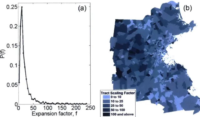
to designated home stays are filtered out. This filter serves the additional purpose of ensuring with a reasonable degree of certainty that the designated stay is the user's home, a key assumption in our method of upscaling users to population. Note that this filtering process necessarily excludes visitors, for whom a home location is not observed in the studied dataset. Future research could look at extracting visitor trips from CDR data using an assumption other than home location to upscale these trips. After this filtering, 335, 795 users remain in the Boston CDR dataset. This sample size is an order of magnitude larger than in most household travel surveys, and should increase given longer periods of observation. To upscale these users to total population of the study region, the number of home stays were aggregated to the 974 Census tracts in the study area. An expansion factor was then calculated for each tract as the ratio of the 2010 Census population and the number of residents identified in the CDR data. For the 10 Census tracts with fewer than 10 CDR residents, the scaling factor is set to 0 to ensure that we don't overweight users that are not representative of a given Census tract. The 1st, 2nd, and 3rd quartiles of the expansion factors are 9.4, 14.2, and 25.1, respectively, as illustrated by the tight probability distribution of expansion factors in Figure 2-2a. The spatial distribution illustrated in Figure 2-2b suggests that the tracts in the western portion of the study area tend to be more heavily weighted. CDR data for a period greater than 60 days would likely have lower expansion factors and an improved spatial distribution of users, however, we show that already this limited data set gives reasonable results.

2.3.4 Trip Estimation

With stays for each user designated by activity type and expansion factors to upscale users to population, average daily origin-destination trips can be constructed by time of day and purpose-home-based work (HBW), home-based other (HBO), and non-home based (NHB). This segmentation allows us to capture distinct trip-making patterns and is consistent with segmentation in the trip distribution stage of trip-based travel demand models.

(36)

0.25 0.2 0.15 0L 0.1. 0.05 j"0 to 10 0 Mi=~en 0 ton2 0 50 100 150 200 250 25o50 Expansion factor, f 100 .m.W..

Figure 2-2: (a) Probability distribution of Census tract expansion factors. (b) Thematic map showing the spatial distribution of Census tract expansion factors.

(based on phone usage) rather than true arrival time and duration of a user, we infer trip departure hour using probability density functions to account for this uncertainty. The publicly-available 2009 National Household Travel Survey (NHTS) [84], filtered for respondents residing in a consolidated metropolitan statistical area (CMSA) or

MSA with populations greater than or equal to 3 million, is a reasonable source as

it approximates temporal travel patterns of major US cities comparable to Boston, while allowing for transferability of this methodology to other US cities. Using this departure time data, we generate six hourly distributions for weekdays and weekends and the following trip purposes: HBW, HBO, and NHB.

For each user, it is assumed that a trip is made between two consecutive stays (i, i+

1) occurring within a 24-hour period beginning and ending at 3am. The trip occurs at

a point in time spanned by the range [si +6, si+] , where s is the observed arrival time and 6 is the observed duration of a stay. The departure hour is randomly generated in this time window using the NHTS distribution that corresponds to the day (weekday, weekend) and the trip purpose identified from the origin and destination stay activities

(37)

(HBW, HBO, NHB).

Furthermore, it is presumed that a user starts and ends each 24-hour period at home such that if a user is not recorded at his/her home stay for the first (last) record of the 24-hour period, his/her first (last) trip begins (ends) at his/her home stay. The first (last) trips are assumed to occur at point in time spanned by the range [3AM, s+1] (fsi + 6 _,_{3AMJ), where s is the observed arrival time and 6 is the}

observed duration of a stay. As before, the departure hour is randomly generated in this window using the NHTS distribution that corresponds to the day (weekday, weekend) and the trip purpose based on the destination (origin) stay activity (HBW, HBO).

Through this process, we construct trips on all days we observe each user. The frequency of weekday observations per user is illustrated in Figure 2-3. The distribu-tion of total weekday trips per user is shown in Figure 2-3a, with first, second, and third quartiles of 33, 58, and 96 trips, respectively. The reindexing of anonymous user IDs mentioned previously in Section 2.2 is evident in the two peaks of the distri-bution of the number of weekday days we observe each user, as seen in Figure 2-3b. Despite this reindexing, we achieve a sufficiently large number of observation days per person, with first, second, and third quartiles of 11, 17, and 21 days, respectively. Dividing each user's total weekday trips by his/her total weekday days, we get the distribution of average weekday trips shown in Figure 2-3c. The distribution has a long tail, however, the first, second, and third quartiles are 2.6, 3.2, and 4.3 average trips per weekday, respectively, demonstrating that the vast majority of users have a reasonably small number of daily trips.

In order to obtain average daily OD trips, each user's trips are multiplied by the expansion factors described in Section 2.3.3 for the user's home Census tract and divided by the number of days from which we constructed the user's trips. For users assigned a work stay, weekday trips are only constructed on days in which the user is observed at his/her work stay to ensure we capture representative weekdays of commuters. Unlike traditional travel surveys which ask a respondent details about one or a few recent days, this method has the advantage of capturing many days per

(38)

o (a) (b) M (c)

08

0 0

Total Weekdy Trips T Tota Weeday Days, D Avrge Weekda Tris t Figure 2-3: Frequency of weekday observations per user. (a) Probability distribution of total weekday trips per user. (b) Probability distribution of total weekday days per user. (c) Probability distribution of average weekday trips per user.

user and thus variations in his/her daily travel behavior. Lastly, each user's average daily trips are aggregated into Census tract pair trip matrices by day type (weekday, weekend), purpose (HBW, HBO, NHB), and hour of departure.

2.4 Results and Validation

2.4.1 Productions and Attractions

Accurately extracting and upscaling users' stays is crucial to trip generation. Due to the regularity of human behavior [78, 77, 40], we are able to infer users' home and (if applicable) work stay locations from CDR data. For this dataset, we find that we can reasonably represent the spatial distribution of home and work locations when aggregated to the 164 study area cities and towns [551. Refer to Section 2.4.2 below for more information on the impact of aggregation level on accuracy. Figure 2-4a shows a comparison of home locations by town from 2010 Census data and the raw and upscaled CDR data.

As we would expect since tract population was used to upscale the data, the number of residents in each town is almost identical to that of the upscaled CDR data. However, the slope of a best-fit line through the raw CDR data is close to 1, which speaks to the fact that the overall distribution of raw CDR users is fairly rep-resentative and a simple factoring method is in fact appropriate to expand the phone

(39)

// / 7 10 16 (a) 10 S3 10 10 10 -no U) CL 0 3: I0 77 10 7 6 t (b) 10 10-10 4-* 10 101 Scaled CDR Raw CDR 10 11 12 13 14 15 6 7 W'0 1 2 3 4 5 6 7 10101010101 10 10 10 10 10 10 10 10 10 10 CDR Residents CDR Workplaces

Figure 2-4: (a) CDR residents vs. 2010 Census population by town before and after pop-ulation expansion. (b) CDR vs. Census Transportation Planning Products (CTPP) [85] workers by town before and after population expansion.

users to population. Similarly, Figure 2-4b shows a comparison of work locations aggregated by town. As with the raw CDR data on the home-end, the distribution of raw workplaces is fairly consistent with the 2006-2010 Census Transportation Plan-ning Products (CTPP) [85] data (slope approximately 1), and the upscaling method adjusts well for the difference in magnitude. This strong correlation is noteworthy considering that each users' home and work locations were scaled based on their home location only.

2.4.2 Trip Distribution

With the establishment of reasonable distributions of trip productions and attractions, we next validate the distribution of trips using two local surveys. The 1991 Boston Household Travel Survey (BHTS) contains information on 39, 300 trips made by 3, 737 households [17], while the 2010/2011 Massachusetts Travel Survey (MHTS) contains data on 153, 099 trips made by 32, 739 people [61]. We find that the CDR trips compare well with trips from these data sources by time of day and purpose. Figure 2-5 illustrates the distributions of hourly departure times for (a) HBW, (b) HBO,

- Scaled CDR Raw CDR C 0 L-0. ~

Cell phone location data for travel behavior analysis

Cell Phone Location Data for Travel Behavior

Analysis

by

Lauren P. Alexander

B.S., University of Texas at Austin (2009)

ARCHNE8

JUL 02 2015

LIBRARIES

Submitted to the Department of Civil and Environmental Engineering

in partial fulfillment of the requirements for the degree of

Master of Science in Transportation

at the

MASSACHUSETTS INSTITUTE OF TECHNOLOGY

June 2015

@

Massachusetts Institute of Technology 2015. All rights reserved.

Author.

A u h

r ..

...

...

...

...

...

...

...

...

....

Signature redacted

Signature redacted

C ertified by

...

Accepted by...Signature

redacted

Heidi M. N pf

Cell Phone Location Data for Travel Behavior Analysis

Abstract

Acknowledgments

Contents

List of Figures

117],

>

List of Tables

Chapter 1

Introduction

1.1

Overview and motivation

1.2

Literature review

1.2.1

Transportation engineering

Schedule

Tours

Trips

w

w

158],

135].

19,

1.3

Outline

Chapter 2

Inferring origin-destination trips by

purpose and time of day

2.1

Introduction

170,

/trajectories

[45].

2.2

Data Description

2.3

Data Processing

2.3.1

Stay Extraction

2.3.2

Activity Inference

2.3.3

Filtering and Expansion

_{A u h}

_{r ..}

_...

_...

_...

_...

_...

_Tours

_Trips