Publisher’s version / Version de l'éditeur:
Vous avez des questions? Nous pouvons vous aider. Pour communiquer directement avec un auteur, consultez la première page de la revue dans laquelle son article a été publié afin de trouver ses coordonnées. Si vous n’arrivez Questions? Contact the NRC Publications Archive team at
[email protected]. If you wish to email the authors directly, please see the first page of the publication for their contact information.
https://publications-cnrc.canada.ca/fra/droits
L’accès à ce site Web et l’utilisation de son contenu sont assujettis aux conditions présentées dans le site
LISEZ CES CONDITIONS ATTENTIVEMENT AVANT D’UTILISER CE SITE WEB.
Third International Conference on CFD in Minerals and Process Industries
[Proceedings], 2003
READ THESE TERMS AND CONDITIONS CAREFULLY BEFORE USING THIS WEBSITE.
https://nrc-publications.canada.ca/eng/copyright
NRC Publications Archive Record / Notice des Archives des publications du CNRC :
https://nrc-publications.canada.ca/eng/view/object/?id=96039884-e210-4c72-b0c9-d4f492061e2a
https://publications-cnrc.canada.ca/fra/voir/objet/?id=96039884-e210-4c72-b0c9-d4f492061e2a
NRC Publications Archive
Archives des publications du CNRC
This publication could be one of several versions: author’s original, accepted manuscript or the publisher’s version. / La version de cette publication peut être l’une des suivantes : la version prépublication de l’auteur, la version acceptée du manuscrit ou la version de l’éditeur.
Access and use of this website and the material on it are subject to the Terms and Conditions set forth at
Performance predictions in solid oxide fuel cells
Third International Conference on CFD in the Minerals and Process Industries CSIRO, Melbourne, Australia
10-12 December 2003
Performance Predictions in Solid Oxide Fuel Cells
Yongming LIN and Steven BEALE
National Research Council, Ottawa, Ontario, K1A 0R6, CANADA
ABSTRACT
This paper describes a program of numerical analysis of planar solid oxide fuel cells and stacks of fuel cells. The solid oxide fuel cell is a solid-state device which converts chemical energy to electricity and heat. We have developed several models of these devices, using commercial computational fluid dynamics packages, and also an in-house programs. In a fuel cell, complex multi-physics and chemistry phenomena interact with transport processes. The ideal electric potential is a function of the fuel and oxidant concentrations, temperature, and pressure. The actual potential is less than the theoretical value due to kinetic, mass transfer and electrical losses. Current density is dependent on both voltage and cell resistance. Sources and sinks of mass, species and heat, are a function of current density. Thus the transport problem is fully-coupled. NOMENCLATURE D diffusion coefficient F Faraday’s constant '' i current density '' 0
i exchange current density k permeability M molecular weight n number of electrons p pressure S source term u velocity x molar fraction m mass fraction α transfer coefficient G
∆ Gibb’s free energy of formation
H ∆ enthalpy of formation ε porosity Φ electrical potential η activation overpotential Ω
η Ohmic voltage loss
µ dynamic viscosity
ρ gaseous mixture density
σ electrical conductivity
τ torosity
INTRODUCTION
Fuel cells combine hydrogen-rich fuel with oxygen to generate electricity, water, and heat. The fuel cell was invented by Grove in 1839, and the first alkaline fuel cell prototype developed by Bacon in 1932 (Berger, 1968). The high energy efficiency and apparent environmentally-benign attributes make fuel cells a candidate for future power sources. Thus, in the last two decades, commercialization of fuel cells has become important, with the development of new technologies to overcome the major technical and cost barriers for this technology.
These developments have stimulated progress in fuel cell modelling and numerical analysis: Computational fluid dynamics (CFD) is playing an important role in assisting fuel cell manufacturers design products, and speed up the development process. The solid oxide fuel cell (SOFC) operates at 800-1000°C and is considered a potential source for stationary and other applications. The solid-state electrolyte is made from zirconia, a brittle material, which is liable to crack under sufficient stress. Numerical simulation tools are used to simulate the temperature and thermal-induced stress distribution to ensure the integrity of the SOFC design, as well as overall predictors of the device performance.
From publication of early SOFC models (Vayenas and Hegedus, 1985), SOFC modelling techniques have advanced significantly, with models at micro-scales and macro-scales being developed. Microscopic models are aimed at building better electrodes and electrolyte, while macroscopic models target stack optimisation.
The physical-chemical transport phenomena within fuel cells are complex, and so are the mathematical and corresponding numerical methods presently employed. These include convection-diffusion of multi-species gas mixtures in micro-channels and porous media, heat and mass transfer due to electrochemical reactions and associated Ohmic heating, as well as kinetic (activation) terms. Ideally, numerical calculations should reproduce all the above mentioned phenomena faithfully. For this, the demand for computer resources is significant. Fine meshing in near wall region may not be feasible for large-scale designs: To alleviate this, simplified models have also been developed. Beale et al. (2001) proposed two alternative numerical models, namely the a CFD-based distributed resistance analogy (DRA) and a non-CFD
based presumed (upstream) flow method (PFM). These assume momentum/heat and mass transfer may be estimated by introducing appropriate drag, and heat and mass transfer coefficients. These simplified approaches have been verified and proven to be realistic alternative to more demanding detailed CFD numerical simulations. In this paper further developments to both detailed and simplified transport models are presented and discussed.
MODEL DESCRIPTION
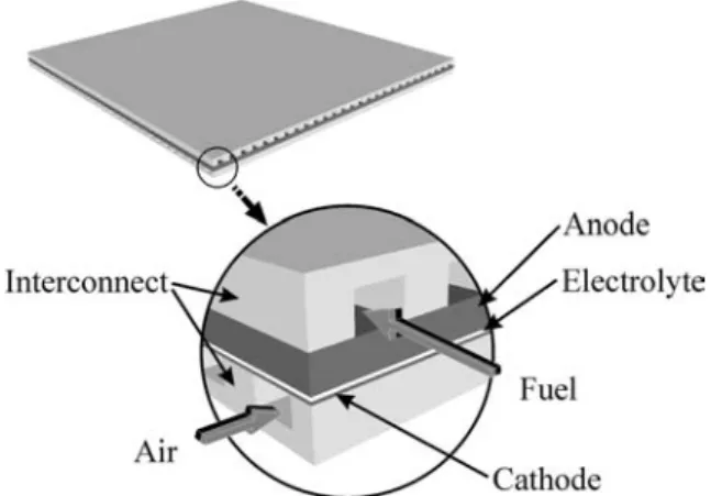
The geometry of the SOFC considered in this study is shown in Figure 1. The basic unit is composed of seven (7) layers in the vertical direction (from bottom-to-top): (1) air-side interconnect (current collector); (2) air-side gas micro-channels, (3) porous cathode, (4) electrolyte, (5) porous anode, (6) fuel-side gas micro-channels, and (7) interconnect on fuel side. Air and fuel are introduced to the micro-channels via manifolds (not shown). Material properties are listed in Table 1. Figure 2 shows the dependence of resistance vs. temperature for the material used for the electrolyte (yttria-stabilized zirconia).
The physical-chemical transport phenomena in a SOFC are strongly coupled. For convenience, we classify them into the following categories: (i) Mass transfer in gas channels and porous media; (ii) Heat transfer in all constituent materials; (iii) Electrochemical reactions at interfaces between electrolyte and electrodes; (iv) Electronic and ionic charge transfer through solid and porous media.
Mass transfer
Convective mass transfer plays an important role in the micro-channels, where the Navier-Stokes equations govern the velocity distributions. The species conservation equation is
(
ρ m)
−∇⋅(
ρD∇m)
=S''' ⋅∇ u (1)
ρ is the mixture density, m is mass fraction, u is local velocity, D is the diffusion coefficient, S is a ''' volumetric source term,
Darcy’s law may be applied to the porous electrodes,
p k ∇ εµ − = K u (2)
Mass transfer in the porous electrodes may be written in the same form as equation (1), but based on an effective diffusion coefficient D , defined by eff
τ
ε
= D
D
eff (3)where τ is ‘tortuosity’, and ε porosity.
At the interface between the porous electrodes and the electrolyte, the source/sink term per unit area, S’’, for a given species (reactant/product) may be written,
''
'' i
nF M
S =± (4)
where M is molecular weight, n the number of electrons involved in the electrochemical reaction, F is Faraday’s constant and ''i is the local current density at the
interface.
Figure 1. Anode supported SOFC geometry considered in present study
Heat Transfer
Convective heat transfer is the dominant transfer mechanism in the micro-channels, while conduction governs the heat flux distribution within solid materials; the current-collecting interconnects, the porous electrodes and the electrolyte.
For the electrochemical reaction,
O H O H2 2 2 2 1 → + (5)
The total energy change resulting from the above reaction is the difference in enthalpy of formation H∆ and Gibb’s energy of formation G∆ , which is (theoretically) converted into electricity, the remainder of it is converted into heat. In reality, electrical (Ohmic) and activation (ki`netic) losses, more chemical energy is irreversibly converted into heat, rather than electricity. Thus if V is the operating voltage, the overall heat source may be written as, ∆ − = V nF H i S (6)
Equation (6) includes heat generated due to all sources. It does not however provide any indication as to how these terms are computed.
Adiabatic boundary conditions are applied the outer walls, ie all heat is removed by the air and fuel. Inlets velocity values are determined from prescribed utilization rates for fuel and air; 25% for oxygen and 50% for hydrogen.
Electrochemistry
Equation (5) may be written in terms of half-reactions
− → +2e 2O O2 (7) O H e 2 O H2+ − → 2 − (8)
Thickness (mm) Resistivity (Ω cm) Thermal conductivit y (W/cm K) Anode 0.1 0.001 0.11 Electrolyte 0.1 Fig. 2 0.027 Cathode 1.0 0.013 0.02 Interconnect 1.143 0.5 0.02
Table 1: Physical properties of materials in SOFC. The first reaction is endothermic and the second exothermic. Since the electrolyte is a very thin layer, it is acceptable to take the two reactions as one. These reactions take place on either side of the electrolyte. The Nernst potential may be written as follows,
a O H O H P nF RT x x x nF RT E E ln ln 2 2 2 2 1 0 + + = (9)
Equation (9) determines the maximum thermodynamically-possible cell voltage. However, if the current density value ''i is greater than the exchange current density ''i0 , there would be voltage reductions,η,
due to activation (kinetic) losses. The activation overpotential is written in the form of a Butler-Volmer equation as follows,
(
)
− −α η − α η = RT nF RT nF i i'' 0'' exp exp 1 (10)where α is a transfer coefficient, 0<α<1. A value of 5
. 0 =
α , and a constant value of i0''=2000 A/m
2 for
cathode (Chan, Khor and Xia, 2001) were selected. Anodic losses were considered negligible.
Electric potential
Electronic conduction in the solid materials (metallic interconnects, and porous electrodes) is governed by the following equation,
( )
σ∇Φ =0 ⋅∇K K (11)
where σ is the electrical conductivity, and Φ is the potential. The local current density vector may be computed according to Ohm’s law as,
Φ ∇ σ − = K '' i (12)
It is assumed that no electron flow through the electrolyte. Since the electrolyte is a thin layer, a quasi one-dimensional (1-D) approach is considered appropriate for the potential in the ionically-conducting electrolyte layer. The electrodes are thus taken to be perfect electrical conductors, so the potential at the electrode-electrolyte interface is constant . 600 700 800 900 1000 0 50 100 150 200 250 300 350 400
Figure 2. Electrolyte resistivity computed according to (Nagata, et al., 2001)
The cell voltage, V, may thus be expressed as,
∑
− η − η − =E i R Vcell a c '' (13)where ηa and ηc are the activation overpotentials on the anode and cathode sides,
∑
i ''Ris the sum of all resistive losses; ionic (electrolyte) and electronic (interconnects, electrodes).The potential difference between the anode and cathode is just Vac=E−ηa−ηc−i''Re, where only Ohmic losses in the electrolyte are considered.A locally 1-D model is presumed. Integrating, the following expression is obtained,
(
)
∫
∫
−η −η − ⋅∫
= dA R dA I dA E R V eletrolyte avg c a e electrolyt ac 1 1 (14)which provides a convenient means for adjusting the potential to achieve the desired mean current (density). At electrolyte-electrode interfaces, it is further presumed that,
e electrolyt electrode i n = '' ∂ Φ ∂ σ − (15)
The resistivity of the electrolyte strongly depends on the temperature, and their relationship could be written as, as shown in The resistivities of other layers are assumed constant as their weaker dependence on temperature then the electrolyte layer.
Constant electrical potential is defined at both the top and bottom walls. 0 potential value is assigned to the top wall, which potential value is adjusted in such a way that consistency in potential values is ensured at the interface between the cathode and electrolyte.
R (Ω ) T (°C) − + = 1273 1 15 273 1 10100 exp 0 T R Re e
680 700 720 740 760 780 800 800 820 820 840 3200 3500 3500 3800 3800 4100 4400 4400 4700 5000
Figure 3. Temperature (°C) at ''i =4,000A/m2. Figure 4. Electrolyte current density, i = 4,000A/m'' 2
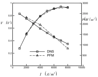
0.116 0.114 0.118 0.120 0.122 0.124 0.126 0 2000 4000 6000 8000 10000 0 0.2 0.4 0.6 0.8 1 0 500 1000 1500 2000 2500 3000 DNS PFM
Figure 5. Oxygen mass fraction distribution. Figure 6. Polarization curve.
Fuel Interconnect Anode Electrolyte -0.04 -0.037 -0.034 -0.031 -0.028 -0.025 -0.022 -0.019-0.016 -0.01 -0.007 0.004 -0.004 -0.001 -0.001 Anode Fuel Interconnect
Figure 7. Current density field around fuel channels. Figure 8. Electrical potential around fuel channels. Air F l
(
A/ m2)
I(
W m2)
P( )
V V ll Fuel Air Fuel AirInterconnect Air
Cathode Electrolyte
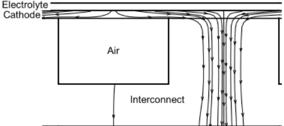
Figure 9. Current density field around air channels.
RESULTS AND DISCUSSION
Detailed numerical simulations were conducted with a commercial CFD code, Fluent. The electrochemistry, transport and electric potential models, described above were implemented by means of user defined functions. Also, a C++ code, based on presumed constant flow at the inlet(s) to the cell, was developed in-house.
SOFC Performance Predictions
Ideally, the SOFC would be at uniform temperature, minimising thermally-induced stresses. The practical situation is, however, not so simple, and the temperature varies substantially within the electrolyte as shown in Fig. 3. It can be seen the difference between the maximum and minimum temperature is approximately 200°C and that the highest temperature is located near the air outlet. In general, higher overall temperatures occur at higher current densities, a smight be expected.
Figure 4 shows the current density distribution at the interface between the anode and the electrolyte. It can be seen that the current density is not distributed uniformly. The current density distribution is affected by the hydrogen and oxygen distributions, Fig. 5, and also by the temperature-dependent electrolyte resistance, Fig. 2: Figure 6 shows polarisation curves for 50% utilization rate for hydrogen and 25% of oxygen. These are obtained for both the detailed CFD code and the simplified C++ code developed in this programme of research. It can be seen that agreement between the codes is satisfactory.
The V-i’’ polarization curve is a standard performance measure for every SOFC/stack. A typical polarization curve is identified by the 3 regions; activation (kinetic), Ohmic and concentration (mass transfer) controlled regions. At high temperature, voltage losses due to activation are small, Eq. (10), and this section of polarization curve is not apparent in high-temperature SOFC’s as in low temperture fuel cells, such as protn exchange membrane fuel cells. For the present case, a large part of the V-i’’ curve is dominated by Ohmic losses. Optimum power density and electrical efficiency are thus determined by the resistance to oxygen ions across the electrolyte. Thus, higher working temperatures, or a
thinner electrolyte would lower the overall resistance, and hence improve the performance of the unit.
Figure 6 also shows the average power density variation as a function of local current density. The maximum power output occurs at the averaged current density equal to 7500 A/m2.
Electric Potential Distribution
Local current density and electric potential distribution within a SOFC are illustrated in Figs. 7 and 8. The anode serves as a diffusion layer for hydrogen. The electric potential distribution determines the local current density, and the prediction of potential distribution can provide the following information to the designer: (1) The effect of rib width on current density distribution at the electrolyte interface and on the cell voltage due to ohmic losses across the interconnects. (2). The effect of the electrode thickness on Nernst potential, and activation overpotentials at the electrolyte interface.
Figure 7 shows flux lines of current density in the fuel-side interconnect. The effect of the rib width on the current density distribution within the interconnector can be seen. At the top plane of the interconnect, local current density values vary due to the rib locations. Figure 8 shows the electrical potential distribution around the fuel channels. It can be seen that the iso-potential lines are perpendicular to the fuel channel walls. Higher current densities occur in areas where the iso-potential lines are more densely distributed. Local current density and electrical potential variations affect the interconnect Ohmic losses and the Ohmic heat source terms, and thus influence the temperature distribution.
The cathode (not shown) serves as a diffusion layer for oxygen. However, for the present geometry, Fig. 1, it is thin compared to the anode. Thus, at sufficiently large current density, the oxygen diffusion flux is insufficient to provide the required oxygen. The current density is thus small in the areas between neighbouring air channels, where the least fuel mass fraction is located.
Code comparison
Comparison between the CFD-based detailed numerical simulations and the presumed inlet flow (non-CFD) is positive. In addition to the polarisationa nd power density characteristics, Fig. 6, comparison of the temperature and mass fraction distributions (not shown) were encouraging. There are two or even three different effects could come to play in terms of species mass fraction distributions: the Darcy pressure-forced convection, mixture mutual diffusions, and or Knudson diffusion.
CONCLUSIONS
The performance of a SOFC relies on the local Ohmic resistance of the electrolyte, which is a function of the temperature distribution and hence the current density (ie. power dissipation). While ideally, evenly distributed temperature and current density distributions are desired, in practice these may not be attainable in present-day designs.
Comparisons between the detailed-CFD calculations and simpler presumed (inlet) flow approaches suggest simplified methods can, under many circumstances be used to give reliable predictions of the performance of SOFC’s as well as traditional detailed CFD methodologies. Comparisons between the results of these two approaches show remarkable similarity in terms of temperature, current density and species mass fraction distributions. Polarisation curves also compare in a favourable manner.
While judicious design of the porous electrodes and electrolyte of a SOFC could greatly improve the electrical performance. Other parameters, such as temperature and current density distributions, also play important roles in determining the SOFC performance. Moreover, for the type of anode-supported SOFC considered in the present study, the current density distribution is strongly dependent on the oxygen mass fraction distribution in the cathode.
Predictions of the electric potential distribution made using the detailed CFD code show revealed the current flow paths through the bi-polar plates (interconnects) and the electrodes. The electric field potential and current density distribution through these layers affects the rates at which electro-chemical reactions take place, and the overall performance of the SOFC.
REFERENCES
APPLEBY, A.J. and FOULKES, F.R., (1989), Fuel Cell
Handbook, Van Norstrand Reinhold, New York.
BERGER, C. (1968), Handbook of Fuel Cell
Technology, Prentice-Hall, England Cliffs, N.J.
BEALE, S.B., DONG, W., ZHUBRIN, S.V., and BOERSMA, R.J., (2001), "Calculations of Transport Phenomena in Stacks of Solid-oxide Fuel Cells",
Proceedings, ASME International Mechanical Engineering Congress and Exposition,
IMECE2001/PID-25615, New York, November 11-16.
CHAN, S.H., KHOR, K.A. and XIA, Z.T., (2001) “A complete polarization model of a solid oxide fuel cell and its sensitivity to the change of cell component thickness”,
Journal of Power Sources, 93, 130-140.
NAGATA, S., MOMMA, A., KATO, T. and KASUGA, Y., (2001), “Numerical analysis of output characteristics of tubular SOFC with internal reformer”, Journal of
Power Sources, 101, 60-71.
VAYENAS, C.G., and HEGEDUS, L.L., (1985), “Cross-Flow, Solid-State Electrochemical reactors: A Steady-State Analysis”, Industrial & Engineering