Time-resolved observation of the Eigen cation in liquid water

(1)

HAL Id: hal-00824061

https://hal-polytechnique.archives-ouvertes.fr/hal-00824061

Submitted on 5 May 2014

HAL is a multi-disciplinary open access

archive for the deposit and dissemination of

sci-entific research documents, whether they are

pub-lished or not. The documents may come from

teaching and research institutions in France or

abroad, or from public or private research centers.

L’archive ouverte pluridisciplinaire HAL, est

destinée au dépôt et à la diffusion de documents

scientifiques de niveau recherche, publiés ou non,

émanant des établissements d’enseignement et de

recherche français ou étrangers, des laboratoires

publics ou privés.

Time-resolved observation of the Eigen cation in liquid

water

Wafa Amir, Guilhem Gallot, François Hache, S. Bratos, J.-C. Leicknam, R.

Vuilleumier

To cite this version:

Wafa Amir, Guilhem Gallot, François Hache, S. Bratos, J.-C. Leicknam, et al.. Time-resolved

obser-vation of the Eigen cation in liquid water. Journal of Chemical Physics, American Institute of Physics,

2007, 126 (3), pp.34511. �10.1063/1.2428299�. �hal-00824061�

(2)

Time-resolved observation of the Eigen cation in liquid water

Wafa Amir, Guilhem Gallot, François Hache, S. Bratos, J.-C. Leicknam, and R. Vuilleumier

Citation: The Journal of Chemical Physics 126, 034511 (2007); doi: 10.1063/1.2428299 View online: http://dx.doi.org/10.1063/1.2428299

View Table of Contents: http://scitation.aip.org/content/aip/journal/jcp/126/3?ver=pdfcov Published by the AIP Publishing

Articles you may be interested in

Time-resolved spectroscopy of silver nanocubes: Observation and assignment of coherently excited vibrational modes

J. Chem. Phys. 126, 094709 (2007); 10.1063/1.2672907

Femtosecond time-resolved investigation of the vibrational modes of vitreous Ge O 2 Appl. Phys. Lett. 89, 251913 (2006); 10.1063/1.2420775

Time-resolved observation of intermolecular vibrational energy transfer in liquid bromoform J. Chem. Phys. 112, 6349 (2000); 10.1063/1.481195

Time-resolved Raman spectroscopy of polytetrafluoroethylene under laser-driven shock compression Appl. Phys. Lett. 75, 947 (1999); 10.1063/1.124563

Use of time-resolved Raman scattering to determine temperatures in shocked carbon tetrachloride J. Appl. Phys. 81, 6662 (1997); 10.1063/1.365206

(3)

Time-resolved observation of the Eigen cation in liquid water

Wafa Amir,a兲 Guilhem Gallot,b兲and François Hache

Laboratoire d’Optique et Biosciences, Ecole Polytechnique, CNRS, INSERM, 91128 Palaiseau, France

S. Bratos, J.-C. Leicknam, and R. Vuilleumier

Laboratoire de Physique Théorique des Liquides, Université Pierre et Marie Curie, 4 Place Jussieu, 75252 Paris Cedex 05, France

共Received 23 June 2006; accepted 5 December 2006; published online 18 January 2007兲

Experimental observation and time relaxation measurement of the hydrated proton Eigen form 关H3O+共H2O兲3兴 are presented here. Vibrational time-resolved spectroscopy is used with an original

method of investigating the proton excess in water. The anharmonicity of the time-resolved spectra is characteristic of the Eigen-type proton geometry. Proton relaxation occurs in less than 200 fs. A calculation of the potential energy confirms the experimental result and the Eigen cation lifetime is in good agreement with previous molecular dynamics simulations. © 2007 American Institute of

Physics.关DOI:10.1063/1.2428299兴

I. INTRODUCTION

Water is a key element in chemistry and biochemistry and its study is of increasing interest to a large scientific community. In particular, water is the most universal solvent and its role is critical for the chemistry of life. It possesses many puzzling characteristics including the proton mobility which is at least five times larger than for other cations.1,2 This anomalous high mobility plays a dominant role in the acid-base and proton transfer reactions which occur in many important biochemical processes. However, the abnormal proton high mobility in water is still an open question.3,4 In particular, the apparent displacement of proton in water is too rapid to be due to an atomic displacement. A possible explanation of this feature was first suggested by von Grotthuss5 in the 19th century. He proposed a mechanism where the charge, and not the proton itself, is transferred between water molecules. Description of this so-called Grot-thuss mechanism involves two limit forms of proton: a pro-ton delocalized between two adjacent water molecules 共H5O2

+_{, Zundel type兲 and a proton localized on a water}

mol-ecule关H3O+共H2O兲3, Eigen type兴. 6

Infrared experiments and simulations of proton in hydrated crystals as well as in small water clusters confirm the existence of the two limit types.7–9 Extension to solution is not easy, since an infinite number of configurations exist in liquid water. Nevertheless, the fast proton mobility has been thoroughly investigated in the liq-uid phase by computer simulation techniques and molecular dynamics simulations.10–13 In liquid water, the proton does not exchange between two precise water geometries but be-tween two wide classes of water environments. In the fol-lowing, we keep the Eigen and Zundel limit structural motifs in analogy to the symmetry of the two classes of proton-water geometries. Most interestingly, it appears that the

vi-brational energy of the different forms of the hydrated proton H+_共H

2O兲nis not uniformly distributed, enabling hole burning

pump-probe experiments. Recent neutron diffraction14 and x-ray absorption15measurements studied the modification of the hydrogen bonding network in the presence of proton in solution and point out the observation of Eigen and Zundel structural motifs. However, direct experimental evidence of these forms in liquids is very difficult to obtain. Very re-cently, a femtosecond pump-probe experiment studied high concentration solutions of proton in liquid water,16 confirm-ing the ultrafast relaxation processes in the Grotthuss mecha-nism. Two reasons can explain the difficulty of experimental observation. On the one hand, simulations show that the pro-ton can jump from one form to the other one on a subpico-second time scale and it is therefore difficult to isolate either form. On the other hand, even if one form is isolated, the determination of the limit form involved is difficult. Spectro-scopic data on the two forms are only known from simula-tions which reveal that the ion absorption structures are very broad presumably due to ultrafast spectral diffusion. In this article, we demonstrate experimental observation of the Eigen-type limiting form of proton in water using femtosec-ond time-resolved vibrational spectroscopy. First, the use of ultrashort pulses allows us to excite a definite species and follow its evolution before relaxation or conversion. Second, it gives access to the excited-state absorption spectrum which will be critical for excited proton form identification. We carry out time-resolved experiment on a binary mix-ture HCl/ H2O in the 2600– 3000 cm−1range, using low

pro-ton concentration 共below 1M兲 to avoid Coulombic

interac-tion between protons, contrary to a previous study.16

According to molecular dynamics simulation, this spectral range corresponds to the Eigen-type absorption.17 By mea-suring the excited species absorption spectrum and compar-ing it with model quantum calculation, we confirm that we observe the Eigen cation. This direct experimental observa-tion of this proton type provides important informaobserva-tion on its dynamics. In Sec. II, our experimental method for obtaining a兲_{Present address: Colorado School of Mines Physics Department, 1523}

Il-linois St., Golden, CO 80401.

b兲

Author to whom correspondence should be addressed. Electronic mail: guilhem.gallot@polytechnique.fr

THE JOURNAL OF CHEMICAL PHYSICS 126, 034511共2007兲

(4)

the hydrated proton spectrum is described. In particular, the technique of extracting proton information from the water background is thoroughly discussed. Finally, in Sec. III, we present the main experimental results and discuss about the proton spectrum relaxation.

II. FEMTOSECOND VIBRATIONAL SPECTROSCOPY OF HYDRATED PROTON

A. Experimental setup and procedure

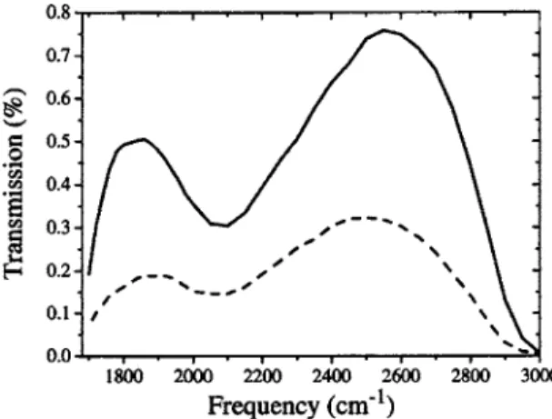
To perform pump-probe hole burning experiments in the midinfrared range, energetic laser pulses are required. The central element of the infrared laser source we used is a titanium-sapphire amplifier, delivering 130 fs pulses at 800 nm with a repetition rate of 1 kHz. It drives two lines of pulses independently tunable in the midinfrared. The prin-ciple of the pulse generation is parametric amplification of a quasicontinuum in the near infrared, followed by frequency mixing in the midinfrared.18The features of the source are as follows. The pump pulses have a duration of 150 fs and a spectral width of 65 cm−1. It delivers more than 10␮J in the 2800– 3800 cm−1 range. The independently tunable weaker line 共the probe兲 has similar characteristics but with a maxi-mum energy smaller than the pump energy by one order of magnitude. The time delay between the pump and the probe is precisely controlled by a computer. The sample cell is 40␮m thick and contains pure water or a solution of HCl in water at room temperature. Typical transmission of pure wa-ter and 0.5M HCl in wawa-ter is presented in Fig.1and shows the important modification of spectral absorption in the pres-ence of the hydrated proton. The sample is circulated to avoid heating problems. The pump and the probe beams are focused in the sample by two 25 mm focal length calcium fluoride lenses. The angle between the pump and the probe beams is 15°. In order to reduce the noise, the probe signal is normalized by a signal tap off the cell. Furthermore, the pump beam is chopped at half the repetition rate of the laser 共i.e., 500 Hz兲, in order to obtain a probe signal with and without the pump. Using this procedure, we achieve a signal to noise ratio of 104_{. For a given pump frequency,}

differen-tial spectra are recorded by tuning the probe frequency for several pump-probe time delays. Typical transmission changes of 10−3 _{are measured. For each probe wavelength,}

we measure the time-resolved differential absorption in pure water and in the HCl solution. This is necessary because pure water gives a large differential signal in this frequency range. This feature has been thoroughly studied recently.19 It is therefore important to be able to extract the signal of the HCl/ H2O solution from the background due to water. Such

an extraction is not straightforward and requires a careful understanding of the origin of the signal in this binary mix-ture. The purpose of the following section is to analyze this question and to come out with a “normalization factor” en-abling us to isolate the relevant signal from the experiment.

B. Calculation of pump-probe signal in binary H2O / HCl mixture

The fundamental difficulty in the study of the proton signature in water is that pure water already exhibits a pump-probe signal, even without proton. Therefore, the system has to be carefully analyzed to suppress the background signal of pure water from the signal measured with the protonated mixture. The following calculations take into account the unusual vibrational properties of pure water in this spectral domain,19 where librational mode plays a major role. Pure water can be described using a four-level quantum system 共see Fig. 2and Ref. 19兲. Pumping it around 2800 cm−1

ini-tiates a transition from the librational state S0 to the first

vibrational excited state S1. From S1, three transitions are

possible: to the ground state共S1→ Sg, bleaching兲, to the

sec-ond excited state 共S1→ S2, induced absorption兲, or back to

the librational state共S1→ S0, bleaching兲. The␯OH frequency

being equal to 3250 cm−1_{, the role of the S}

1→ Sgtransition is

totally negligible, and the ground level Sgwill be neglected

in the following. The plan of our paper is as follows. First, a simple analytical model describing the HCl/ H2O binary

mixture will be presented, using the above assumptions based on the properties of pure water. Next, this simple model will be validated using full rate equation modeling.

1. Simple analytical model

In this model, the water molecule H2O as well as the ion

共H3O兲+are both assimilated to a three-level quantum system

共Fig.2兲. Their total numbers per unit volume are N and N

_⬘

, respectively. The absorption cross sections are ␴1, ␴2, ␴1

⬘

,

and␴₂

_⬘

. Cross sections related to the proton naturally include the contribution of the surrounding water molecules since they belong by definition to the hydrated proton entity. At the submolar HCl concentrations used in the experiments, the

FIG. 1. Transmission spectra through 40␮m of pure water共solid line兲 and 0.5M HCl/ H2O共dashed line兲.

FIG. 2. Energy diagrams for pure water and for solvated proton, with the corresponding cross sections.

034511-2 Amir et al. J. Chem. Phys. 126, 034511 共2007兲

(5)

change of the optical dielectric constant is negligible and does not alter the measurements of the cross sections of the hydrated proton. The sample has a thickness L. The assump-tion of a weak pump flux␾is made. It corresponds to typical experimental conditions and one can assume that ␴1␾Ⰶ 1

and ␴₁

_⬘

␾Ⰶ 1. In the absence of the pump excitation, the transmitted photon flux ␾p is given by the Beer-Lambert

equation

␾_p共z兲 =␾0e−共N␴1+N⬘␴1⬘兲z. 共2.1兲

The pump excitation modifies the populations of different quantum states. The transmitted photon flux for the probe beam is then ␾pp=␾0exp

再

冕

0 L 兵− 关N − ⌬N共z兲兴␴1+ ⌬N共z兲␴1 − ⌬N共z兲␴2其dz

冎

⫻ exp

再

冕

0 L 兵− 关N

⬘

− ⌬N

⬘

共z兲兴␴₁

⬘

+ ⌬N

⬘

共z兲␴1

⬘

− ⌬N

⬘

共z兲␴2

⬘

其dz

冎

, 共2.2兲

where ⌬N and ⌬N

_⬘

designate the number of molecules hav-ing left the ground state for the first excited state. The mea-sured differential pump-probe transmission Tpp=␾pp/␾p is

then T_pp= Tprobe T0 = exp

冕

0 L 关2⌬N共z兲␴1− ⌬N共z兲␴2兴dz ⫻exp

冕

0 L 关2⌬N

⬘

共z兲␴₁

_⬘

− ⌬N

⬘

共z兲␴₂

_⬘

兴dz. 共2.3兲 Let ⌬␴=␴2− 2␴1 and ⌬␴

⬘

=␴2

⬘

− 2␴1

⬘

. One obtains

Tpp= exp

冕

0 L

−关⌬␴⌬N共z兲 + ⌬␴

_⬘

⌬N

_⬘

共z兲兴dz. 共2.4兲 The experimental challenge is then to extract the solute cross section ⌬␴

_⬘

from the total signal. At this point the following assumption is made. One assumes that the ratio

␣= ⌬N

_⬘

共z兲 / ⌬N共z兲 remains constant during propagation through the sample. This implies that the excited populations of the solvent and solute are created in a similar way by the pump. This will be true as long as there is no saturation effect. Validity of this assumption will be numerically dis-cussed later on. Note that兰0

L_{共⌬N + ⌬N}

⬘

兲dz is the total number of excited molecules contained in a cylinder having a basis of 1 m2_{and a length L. This number is equal to the variation}

of the pump flux␾共0兲 −␾共L兲 = ⌬␾. Then

冕

₀L 共⌬N + ⌬N

⬘

兲dz = 共1 +␣兲

冕

0 L ⌬Ndz = ⌬␾. 共2.5兲 Therefore,

冕

₀L 共⌬N⌬␴+ ⌬N

_⬘

⌬␴

_⬘

兲dz =共⌬␴+␣⌬␴

_⬘

兲

冕

0 L ⌬Ndz 共2.6兲 =共⌬␴+␣⌬␴

_⬘

兲 1 1 +␣⌬␾. 共2.7兲

Equation共2.3兲then yields

Tpp= exp

冋

−共⌬␴+␣⌬␴

⬘

兲

1

1 +␣⌬␾

册

. 共2.8兲

Similarly, in the case of pure solvent, i.e., with␣= 0, the relative probe transmission is given by

T_ppw =Tprobe w T0 w = e −⌬␴⌬␾w . 共2.9兲

The differential signals measured in the experiments for the binary solute/solvent and pure solvent are related to these quantities by R= 1 − Tpp, 共2.10兲 Rw_{= 1 − T} pp w .

Since relative transmission changes are small, one can develop these expressions into

R=共⌬␴+␣⌬␴

_⬘

兲共⌬␾/1兲 +␣,

共2.11兲

Rw= ⌬␴⌬␾w

.

We now define a normalization parameter␬ by

␬= ⌬␾ ⌬␾w

1

1 +␣, 共2.12兲

from which the relative transmissions of the solvent and sol-ute may be obtained. There results

S= R −␬Rw= ␣⌬␾

1 +␣⌬␴

⬘

. 共2.13兲

This normalization parameter accounts for the absorp-tion of the solute in the binary mixture: photons absorbed by the solute do not contribute to the solvent excitation, imply-ing that the solvent contribution is less in the binary mixture than in the pure solvent. Under the assumption of a weak pump, the parameter␣can be obtained from the linear

spec-tra of H2O and Haq

+_{. Since ⌬N共z兲 = N}_␴

1␾ and ⌬N

⬘

共z兲

= N

_⬘

␴₁

_⬘

␾,␣= N

_⬘

␴₁

_⬘

/ N␴1, which can be obtained from linear

absorption measurements at 2800 cm−1_{, since the linear}

transmissions for H2O and Haq + are TH共l兲₂O= e−N␴1L, 共2.14兲 T_H aq + 共l兲 = e−N␴1L_e−N⬘␴1⬘L_.

The important point of this calculation is that this nor-malization parameter can be easily obtained from linear

034511-3 Eigen cation in liquid water J. Chem. Phys. 126, 034511 共2007兲

(6)

transmission data at the frequency of the pump in the solvent and in the binary mixture. It is not affected by the physical evolution of the system after excitation and is therefore a robust normalization parameter. In our experimental condi-tions, the parameter ␬ is equal to 0.7. The normalization allows the extraction of ⌬␴

_⬘

=␴₂

_⬘

− 2␴₁

_⬘

, which is the only parameter depending on the probe frequency and which pro-vides the nonlinear pump-probe response of the solute, as in an isolated three-level system.

2. A full three-level quantum system simulation

The above simple model shows that a normalization is possible if the ratio␣defined as ⌬N

⬘

共z兲 / ⌬N共z兲 remains con-stant. We shall now consider a full simulation of the quantum systems, precisely taking into account the excited popula-tions for both solvent and solute, and see if normalization is still possible. If␣ is not constant, then

R= ⌬␴

冕

0 L ⌬N共z兲dz + ⌬␴

_⬘

冕

0 L ⌬N

_⬘

共z兲dz, 共2.15兲 Rw= ⌬␴⌬␾w ,

from which a new normalization parameter␬

_⬘

is obtained:

␬

_⬘

=兰0

L

⌬Ndz

⌬␾ . 共2.16兲

However, ␬

_⬘

depends on how the population evolves,

and it is difficult to evaluate. The question is to know whether, under realistic conditions, the previously defined parameter ␬ is a good approximation to ␬

_⬘

. Full rate equa-tions for solvent populaequa-tions are given by

⳵N0

⳵t =共N1− N0兲␴1F共z,t兲,

共2.17兲

⳵N1

⳵t =共N0− N1兲␴1F共z,t兲 + 共N2− N1兲␴2F共z,t兲,

and for solute populations

⳵N₀

_⬘

⳵t =共N1

⬘

− N0

⬘

兲␴1

⬘

F共z,t兲,

共2.18兲

⳵N₁

_⬘

⳵t =共N0

⬘

− N1

⬘

兲␴1

⬘

F共z,t兲 + 共N2

⬘

− N1

⬘

兲␴2

⬘

F共z,t兲.

Temporal features of the pump now have to be taken into account to fully simulate saturation during pump propaga-tion. Due to the small thickness of the experimental sample, the pump profile remains constant throughout the propaga-tion. Experimental pump pulses are Gaussian, and the tem-poral profile is F共t兲 =

冑

4 ln 2 ␲⌬␶2␾exp

冉

− 4 ln 2 t2 ⌬␶2

冊

, 共2.19兲 where ␾=兰−⬁ +⬁

F共t兲dt and ⌬␶ is the full width at half maxi-mum of the pulse.

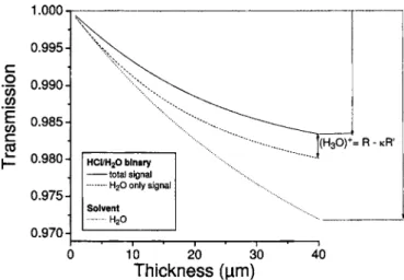
The sample is divided into sections of small thickness. For each section, Eqs. 共2.17兲–共2.19兲are numerically solved to give the resulting population distribution. The energy of the pump is corrected for absorption; then one shifts to the next section. At the end of the simulation, the whole evolu-tion of the populaevolu-tions is known. A typical result is shown in Fig.3, which presents the evolution of the relative transmis-sion of the probe versus the depth of propagation for binary mixture and pure solvent. From the population evolution, one can calculate the evolution of ␣ versus z, as given by Fig.4. Cross sections for pure water are taken from previous work.19Cross sections for solute come from the experimen-tal data. Figures3 and4are calculated for a solute concen-tration of 1% in the number of molecules of hydrated proton with respect to the number of water molecules共0.5M兲. Fig-ure 4 shows the evolution of ␣ with two pump fluxes, re-spectively, 1 ⫻ 1017 _{and 5 ⫻ 10}17_{photons/ cm}2_{. It appears}

that for high flux, ␣ is not constant anymore throughout propagation, which means that evaluation of normalization from linear data is no longer possible. On the contrary, for lower flux,␣is almost constant, and the difference between

FIG. 3. Normalization of binary 共H3O兲+/ H2O mixtures. Relative probe

transmissions are shown vs propagation depth in the sample for binary mix-ture and pure solvent. Solid line: total signal for binary mixmix-ture; dashed line: water contribution to the mixture signal; dotted line: pure solvent. The real contribution from solute can be extracted by normalizing the binary and pure solvent relative transmissions, using normalization coefficient␬.

FIG. 4. Excited population ratio ⌬N_⬘/ ⌬N vs propagation distance for two pump fluxes at 5 ⫻ 1017_{共dotted line兲 and 10}17_{共solid line兲 photons/ cm}2_.

(7)

␬ and␬

_⬘

is very small, less than 1%, and will not affect the quality of the normalization. Pump energy then has to remain under an upper limit, which corresponds to differential probe absorptions below 5%. In our experiments, this condition is fully satisfied and we can safely use the above-defined nor-malization parameter␬.

III. EXPERIMENTAL RESULTS AND DISCUSSION

The differential absorption signals obtained for pump and probe frequencies tuned at 2800 cm−1 _{are displayed in}

Fig.5for pure water and HCl solution共0.5M兲. The similarity between the two signals is a clear indication of the impor-tance of the above-mentioned calculation: most of the solu-tion signal comes from the excited-state absorpsolu-tion in water that was discussed in Ref.19. To investigate the possible role played by the counterion Cl−_{, we also recorded differential}

spectra of NaCl solutions with the same concentration. No measurable difference with respect to pure water has been observed, showing that the presence of the proton is fully responsible for the spectral features of HCl in solution. In order to extract the proton contribution, we apply Eq.共2.13兲

and obtain a neat bleaching of the proton absorption. It is clear from the shape of these curves that the excited state is short lived. However, at that point it is hazardous to try to extract any information because population relaxation, spec-tral diffusion, and laser pulse duration are intricate in this time-resolved signal. This point will be discussed further when the whole spectral response is examined. Similar treat-ment has been performed for 14 probe wavelengths in the 2600– 3050 cm−1 _{range and yielded absorption bleaching on}

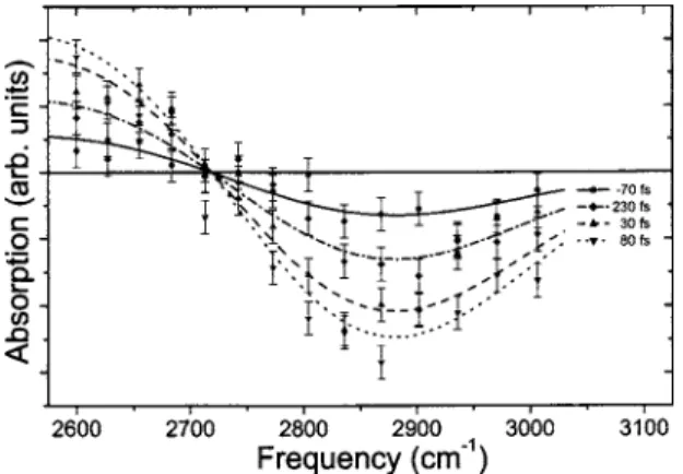
the high-energy side whereas it yielded excited-state absorp-tion on the low-energy one. These findings are summarized in Fig. 6 where the time-resolved spectra of the hydrated proton are displayed for four significant delays: −70, 30, 80, and 230 fs. Several pieces of information can be extracted from these curves. First, all curves have the same shape, indicating that there is no observable spectral diffusion. This feature is consistent with an ultrafast spectral diffusion. The-oretical studies indicate spectral diffusion of hydrated proton to be much faster than the one in pure water, which is less

than 1 ps. It is then probable that such spectral diffusion effects take place on a rapid time scale not accessible to the experiment. Note that such very rapid energy redistribution has been observed in pure water.19,20 Second, this spectral shape with a low-energy excited-state absorption and a high-energy bleaching is characteristic of three-level quantum sys-tems displaying a negative anharmonicity, that is to say that the first excited-state absorption is redshifted compared to the ground state one. As discussed below, this feature is a signature of Eigen-type proton. Finally, we can extract from these spectra a more precise information on the relaxation time of the excited proton. For that, we begin with fitting the induced-absorption structures with Gaussian functions and then plot the band areas as a function of time. The result is displayed in Fig.7. Because the band areas are directly con-nected to the density of excited protons, this curve allows one to extract the population relaxation time despite the band shifts. By applying the procedure exposed in Ref. 21, it is possible to get rid of the pulse duration and to extract the genuine relaxation time. Since no evidence of measurable spectral relaxation is found within the experimental time resolution, the time domain pump-probe data should evolve with the same time scale as frequency domain evolution. An average of time evolution data is then shown in Fig. 7 and

FIG. 5. Differential absorption of HCl共0.5M兲 and H2O as a function of the

pump-probe delay. The pump and probe frequencies are fixed at 2800 cm−1_.

The proton signal共dotted curve兲, extracted with a normalization coefficient 共␬= 0.7兲, displays a bleaching behavior.

FIG. 6. Time-resolved spectra of the hydrated proton in liquid water. The dots represent experimental data with the pump frequency at 2800 cm−1_for

various pump-probe delays共−70, 30, 80, and 230 fs兲.

FIG. 7. Energy relaxation of the excited proton. The round dots are deduced from Gaussian fits of the experimental data. The square dots originate from the averaging of three time domain pump-probe experiments, with probe frequency at 2750, 2800, and 2850 cm−1_{. The lines are calculations for}

different relaxation times.

(8)

provides a better fitting precision at longer delays. The lines in Fig. 7 are fits obtained with this procedure and yield a decay time of 170± 20 fs. Given the low density of proton in the solution, excitation transfer to other protons is not likely to happen. This fast relaxation of the proton vibration is probably due to an efficient coupling with the vibrational modes of the nearby water molecules. These conclusions are in good agreement, within experimental uncertainty, with previous work by Woutersen and Bakker16 and confirm the validity of our normalization procedure. Contrary to this work, we cannot observe a spectral component of the Eigen-type proton at higher frequency, since pure water strongly absorbs above 3100 cm−1.

We now come to the discussion of the negative anhar-monicity observed in Fig. 6. In order to understand the sig-nature of the two proton types共Eigen or Zundel兲 in terms of anharmonicity, we have developed a simple quantum calcu-lation aimed at evaluating the energy potential surface of a hydrated proton interacting with a water molecule共see Fig.

8兲. For the sake of simplicity, we suppose that the three at-oms O¯H¯O are aligned. The potential used in the calcu-lation can be found in the literature.11,22It is issued from an extended quantized empirical valence-bond model for de-scribing the dynamics of an excess proton in water clusters and liquid water,23validated from ab initio and density func-tional theory calculation. It is well suited for the character-ization of the shape of the potential undergone by the proton. The extended model includes all the possible valence states accessible to the excess proton at a given time step and al-lows for a consistent description of the delocalized electronic structure around the excess charge. The potential consists of two parts: an intramolecular potential which accounts for the H3O+molecule and an intermolecular one which deals with

the interaction between H3O+ and H2O. 23

The parameters

can be found in Ref.22. The potential surface of the proton is calculated as a function of the distance ROHtogether with

the corresponding quantum levels, whose variations are ana-lyzed when changing the distance between the two oxygen atoms, ROO. The results are summarized in Fig.8: when the

two oxygen atoms are far apart共typically ROO⬎ 0.3 nm兲, the

proton tends to get localized on one oxygen atom 共Eigen

type兲. The localized proton then moves in a sharp potential well. On the contrary, when the two oxygen atoms are closer 共ROO⬍ 0.26 nm兲, the potential well is much flatter and the

proton wave function is completely delocalized between the two oxygen atoms, which corresponds to the Zundel type. In order to address this point more quantitatively, we have car-ried out quantum mechanical calculation of the first and sec-ond stretching mode frequencies by solving a one-dimensional Schrödinger equation for the O–H coordinate

ROH using the potential previously developed and the

nu-merical Numerov method.24 The striking point is that, look-ing closer at the energy levels, the anharmonicity is negative in the Eigen case, whereas it is positive in the Zundel case. Our experimental finding of a negative anharmonicity there-fore allows us to conclude that it is the Eigen proton that we have observed and demonstrated in our time-resolved experi-ment. Note that this conclusion is in agreement with theoret-ical calculations which predicted that it is the Eigen type which preferentially absorbs at 2800 cm−1.17

IV. CONCLUSION

In this article, we have investigated the ultrafast dynam-ics of proton in pure water by performing femtosecond pump-probe experiment in the 2600– 3000 cm−1_{range. This}

study requires a thorough knowledge of the behavior of wa-ter in this frequency range,19 and the ability to achieve

ul-FIG. 8. 共A兲Geometry of the proton between two water molecules. 关共B兲 and 共C兲兴 Potential energy and energy levels for the Eigen 关共B兲 ROO= 0.3 nm兴 and

Zundel关共C兲 ROO= 0.26 nm兴 ions. The reaction coordinate is the oxygen-hydrogen distance RO–H. The Eigen ion transforms into the Zundel ion by reducing

RO–O. Anharmonicity is negative in the Eigen form and positive in the Zundel form.

(9)

trashort time resolution in this mid-IR range. It permits to monitor the proton in a definite Eigen type before it converts into the Zundel type. We thus observed the excited proton with a relaxation time of 170 fs. Assigning it to the Eigen type was inferred from the negative anharmonicity which is characteristic of the localized form of the proton. This ex-periment should contribute to the elucidation of the von Grotthuss mechanism fundamentals.

1

P. W. Atkins, Physical Chemistry 共Oxford University Press, Oxford, 1997兲.

2

N. Agmon, J. Phys. Chem. A 109, 13共2004兲.

3

N. Agmon, Chem. Phys. Lett. 244, 456共1995兲.

4

J. T. Hynes, Nature共London兲 397, 565 共1999兲.

5

C. J. D. von Grotthuss, Annales de Chimie 58, 54共1806兲.

6

D. Marx, M. E. Tuckerman, J. Hutter, and M. Parrinello, Nature 共London兲 397, 601 共1999兲.

7

J.-W. Shin, N. I. Hammer, E. G. Diken, M. A. Johnson, R. S. Walters, T. D. Jaeger, M. A. Duncan, R. A. Christie, and K. D. Jordan, Science 304, 1137共2004兲.

8

M. Miyazaki, A. Fujii, T. Ebata, and N. Mikami, Science 304, 1134 共2004兲.

9

J. M. Headrick, E. G. Diken, R. S. Walters, N. I. Hammer, R. A. Christie,

J. Cui, E. M. Myshakin, M. A. Duncan, M. A. Johnson, and K. D. Jordan, Science 308, 1765共2005兲.

10

D. Wei and D. R. Salahub, J. Chem. Phys. 101, 7633共1994兲.

11

R. Vuilleumier and D. Borgis, J. Chem. Phys. 111, 4251共1999兲.

12

S. Izvekov and G. A. Voth, J. Chem. Phys. 123, 044505共2005兲.

13

U. W. Schmidt and G. A. Voth, J. Chem. Phys. 111, 9361共1999兲.

14

A. Botti, F. Bruni, S. Imberti, M. A. Ricci, and A. K. Soper, J. Chem. Phys. 121, 7840共2004兲.

15

M. Cavalleri, L.-A. Näslund, D. C. Edwards, P. Wernet, H. Ogasawara, S. Myneni, L. Ojamäe, M. Odelius, A. Nilsson, and L. G. M. Pettersson, J. Chem. Phys. 124, 194508共2006兲.

16

S. Woutersen and H. J. Bakker, Phys. Rev. Lett. 96, 138305共2006兲.

17

J. Kim, U. W. Schmidt, J. A. Gruetzmacher, G. A. Voth, and N. E. Scherer, J. Chem. Phys. 116, 737共2002兲.

18

G. M. Gale, G. Gallot, F. Hache, and R. Sander, Opt. Lett. 22, 1253 共1997兲.

19

W. Amir, G. Gallot, and F. Hache, J. Chem. Phys. 121, 7908共2004兲.

20

M. L. Cowan, B. D. Bruner, N. Huse, J. R. Dwyer, B. Chugh, E. T. J. Nibbering, T. Elsaesser, and R. J. D. Miller, Nature共London兲 434, 199 共2005兲.

21

S. Bratos and J.-C. Leicknam, J. Chem. Phys. 103, 4887共1995兲.