HAL Id: hal-00875641
https://hal.archives-ouvertes.fr/hal-00875641
Submitted on 29 Jan 2020
HAL is a multi-disciplinary open access
archive for the deposit and dissemination of
sci-entific research documents, whether they are
pub-lished or not. The documents may come from
teaching and research institutions in France or
abroad, or from public or private research centers.
L’archive ouverte pluridisciplinaire HAL, est
destinée au dépôt et à la diffusion de documents
scientifiques de niveau recherche, publiés ou non,
émanant des établissements d’enseignement et de
recherche français ou étrangers, des laboratoires
publics ou privés.
Calculations on the EGEE Grid
Antonio Monari, Anthony Scemama, Michel Caffarel
To cite this version:
Antonio Monari, Anthony Scemama, Michel Caffarel. Large-Scale Quantum Monte Carlo Electronic
Structure Calculations on the EGEE Grid. Remote Instrumentation for eScience and Related
As-pects, Springer New York, pp.195-207, 2012, 978-1-4614-0507-8. �10.1007/978-1-4614-0508-5_13�.
�hal-00875641�
structure calculations on the EGEE grid
Antonio Monari, Anthony Scemama, and Michel Caffarel
Laboratoire de Chimie et Physique Quantiques, CNRS-IRSAMC, Universit´e de Toulouse, France,
[email protected], WWW home page: http://qmcchem.ups-tlse.fr
Abstract. A grid implementation of a massively parallel quantum Monte
Carlo (QMC) code on the EGEE grid architecture is discussed. Techni-cal details allowing an efficient implementation are presented and the grid performance (number of queued, running, and executed tasks as a
function of time) is discussed. Finally, we present a very accurate Li2
potential energy curve obtained by running simultaneously several hun-dreds tasks on the grid.
1
Introduction
Quantum Monte Carlo (QMC) methods are known to be powerful stochastic approaches for solving the Schr¨odinger equation.[1] Although they have been widely used in computational physics during the last twenty years, they are still of marginal use in computational chemistry.[2] Two major reasons can be in-voked for that: i) the N -body problem encountered in chemistry is particularly challenging (a set of strongly interacting electrons in the field of highly-attractive nuclei) ii.) the level of numerical accuracy required is very high (the so-called “chemical accuracy”). In computational chemistry, the two standard approaches used presently are the Density Functional Theory (DFT) approaches and the various post-Hartree-Fock wavefunction-based methods (Configuration Interac-tion, Coupled Cluster, etc.) In practice, DFT methods are the most popular approaches, essentially because they combine both a reasonable accuracy and a favorable scaling of the computational effort as a function of the number of electrons. On the other hand, post-HF methods are also employed since they lead to a greater and much controlled accuracy than DFT. Unfortunately, the price to pay for such an accuracy is too high to be of practical use for large molecular systems.
QMC appears as a third promising alternative method essentially because it combines the advantages of both approaches: a favorable scaling together with a very good accuracy. In addition to this, and it is the central point of the present note, the QMC approaches —in sharp contrast with DFT and post-HF methods— are ideally suited to High-Performance-Computing (HPC) and, more specifically, to massive parallel computations either on homogeneous multi-processor platforms or on heterogeneous grid infrastructures. As most “classical”
or “quantum” Monte Carlo approaches, the algorithm is essentially of the num-ber crunching type, the central memory requirements remain small and bounded and the I/O flows are essentially marginal. Due to these extremely favorable computational aspects plus the rapid evolution of computational infrastructures towards more and more numerous and efficient processors, it is likely that QMC will play in the next years a growing role in computational chemistry.
In the present study, the first implementation of our quantum Monte Carlo program on a large scale grid —the European EGEE-III grid[3]— is presented. As a scientific application we have chosen to compute with a very high accuracy the potential energy curve (PEC) of the Li2molecule (total energy of the system
as a function of the Li–Li distance). To the best of our knowlegde, the curve presented here is the most accurate PEC ever published for this system. In order to reach such an accuracy two conditions need to be fulfilled. First, a large enough Monte Carlo statistics has to be realized to reduce the final statistical error down to the precision desired. Second, accurate enough trial wave functions must be employed to reduce as much as possible the so-called “Fixed-Node” error (the only systematic error left in a QMC calculation, see Ref.[2]). The first condition is easy to fulfill since the system is small (only, six electrons) and accumulating statistics is just a matter of making enough Monte Carlo steps and using enough processors (“brute force” approach). The second condition is much more challenging since we need to introduce trial wavefunctions with a controlled nodal quality and which can be improved in a systematic way. Here, we have realized this latter aspect by considering wavefunctions issued from Full Configuration Interaction (FCI) calculations in a large basis-set (technically, the cc-pVQZ basis set, Ref.[4]). Such a FCI trial wavefunction is expected to have a very good nodal structure. However, there is a price to pay: To handle such a function is quite expensive. More precisely, the FCI trial wavefunction used here is expressed a sum of 16,138 products of two 3×3 determinants (three α-electrons and three β-electrons) and, at each Monte Carlo step, this wavefunction and its first- and second- derivatives have to be computed. Note that the computational cost in terms of CPU time is directly proportional to the number of products in the trial wavefunction expansion. To the best of our knowledge, it is the first time that such a high number of determinants in a QMC calculation has been used. Let us emphasize that it has been possible here only because of the use of the grid infrastructure.
In Sec. 2 some technical details related to the implementation of a quan-tum Monte Carlo simulation and the use of our QMC=Chem[5] program are presented. Section 3 presents the computational strategy employed in our appli-cation to the Li2 molecule. Section 4 gives the results and discusses the
perfor-mance. Finally, some conclusions are presented in Sec.5.
2
Technical details
A walker is a vector X of the 3N -dimensional space containing the entire set of the three-dimensional coordinates of the N electrons of the system. During
the simulation, a walker (or a population of walkers) samples via a Monte Carlo Markov Chain process the 3N -dimensional space according to some target prob-ability density (the precise density may vary from one QMC method to another). From a practical point of view, the averages of the quantities of interest (energy, densities, etc.) are calculated over a set as large as possible of independent ran-dom walks. Ranran-dom walks differ from each other only in the initial electron positions X0, and in the initial random seed S0 determining the entire series of
random numbers used.
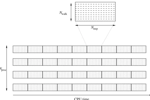
In the QMC=Chem code used here, the main computational object is a block. In a block, Nwalk independent walkers realize random walks of length Nstep,
and the quantities of interest are averaged over all the steps of each random walk. If Nstep is significantly larger than the auto-correlation time (which is
usually rather small), the positions of the walkers at the end of the block can be considered as independent of their initial positions and a new block can be sampled using these configurations as X0 and using the current random seed as
S0.
The final Monte Carlo result is obtained by averaging all the results obtained for each block. If the data associated with each block are saved on disk, the averages can be calculated as a post-processing of the data and the calculation can be easily restarted using the last positions of the walkers and the last random seed.
Note that the computation of the averages does not require any time order-ing. If the user provides a set of Nproc different initial conditions (walker
posi-tions and random seed), the blocks can be computed in parallel. In figure 1, we give a pictorial representation of four independent processors computing blocks sequentially, each block having different initial conditions.
2.1 Design of the QMC=Chem program
The QMC=Chem program was designed specifically to run on heterogeneous clusters via the Message Passing Interface (MPI) API[7] and also in grid envi-ronments via Python[8] scripts. The memory requirements, disk input/outputs and network communications were minimized as much as possible, and the code was written in order to allow asynchronous processes. This section presents the general design of the program.
The behavior of the program is the following. A main Python program spawns three processes: an observer, a computation engine, and a data server (see figure 2).
The observer The observer keeps a global knowledge of the whole calculation (current values of the computed averages, total CPU time, wall time, etc). It updates the results using the calculated blocks at regular intervals of time and checks if the code should continue or stop by informing the data server. It also checks if a stopping condition is reached. The stopping condition can be a max-imum value of the total CPU time, the wall time, the number of blocks, or a threshold on the statistical error bar of any Monte Carlo estimate.
Nstep
Nwalk
Nproc
CPU time
Fig. 1.Graphical representation of a QMC simulation. Each process generates blocks,
each block being composed of Nwalkwalkers realizing NstepMonte Carlo steps.
The computation engine The computation engine starts the Fortran MPI executable. The master MPI process broadcasts the common input data to the slaves, and enters the main loop. In the main loop, the program computes one block and sends the results to the data server via a trivial python XML-RPC client. The reply of the data server determines if the main loop should be exited or if it should compute another block. When the main loop is exited, there is an MPI synchronization barrier where all the slave processes send the last walker positions and their last random seed to the master, which writes them to disk.
A linear feedback shift register (LFSR) pseudo-random number generator[6] is implemented in the code. A pool of 7000 initial random seeds was previously prepared, each random seed being separated from the previous one by 6.1011
seeds. Every time a random number is drawn, a counter is incremented. If the counter reaches 6.1011, the next free random seed is used. This mechanism
guar-antees that the parallel processes will never use the same sequence of random numbers.
The data server The data server is a Python XML-RPC server whose role is to receive the computed data during a simulation and save it into files. Each file is a few kilobytes large and contains the averages of interest computed over a block. The data server also computes an MD5 key[9] related to the critical input values to guarantee that the computed blocks belong to the simulation, and that the input data has not been corrupted.
Generation of the output The output file of the program is not created during the run which only produces block files via the data server. A separate script analyzes the blocks written to disk to produce an output. This script can be executed at any time: while a calculation is running to check the current values, or when the simulation has finished. The consistence between the input data with the blocks is checked with using the previously mentioned MD5 key.
Adaptation to grid environments A script was written to prepare as much files as there are different requested tasks on the grid, each file name containing the index of the task (for example 12.tar.gz). Each file is a gzipped tar file of a directory containing all the needed input data. The only difference between the input files of two distinct tasks is their vector X0 and their random seed
S0. The script also generates a gzipped tar file qmcchem.tar.gz which contains
a statically linked non-MPI Fortran i686-linux executable, and all the needed Python files (the XML-RPC data server, the observer, etc). A third generated file is a shell script qmcchem grid.sh which will run the job.
Another script reverses this work. First, it unpacks all the tar.gz files con-taining the input files and the block files. Then it collects all the block files into a common directory for the future production of the output file.
Termination system signals (SIGKILL, SIGTERM, . . . ) are intercepted by the QMC=Chem program. If any of this signals is caught, the program tries to finish the current block and terminates in a clean way.
2.2 Advantages of such a design
Asynchronous processes Note that the transmission of the computed data is not realized through MPI in the main loop of the computation engine, but with a Python script instead. This latter point avoids the need for MPI synchronization barriers inside the main loop, and allows the code to run on heterogeneous clusters with a minimal use of MPI statements. The main advantage of this design is that if the MPI processes are sent on machines with different types of processors, each process will always use 100% of the CPU (except for the synchronization barrier at the end) and fast processors will send more blocks to the data server than the slower processors.
Analysis of the results The analysis of the blocks as a post-processing step (see section 2.1) has major advantages. First, the analysis of the data with graphical user interfaces is trivial since all the raw data is present in the block files, and they are easy to read by programs, as opposed to traditional output files which are written for the users. The degree of verbosity of the output can be changed upon request by the user even after the end of the calculation, and this avoids the user to read a large file to find only one small piece of information, while it is still possible to have access to the verbose output. The last and most important feature is that the production of the output does not impose any synchronization of the parallel processes, and they can run naturally in grid environments.
Failure of a process As all the processes are independent, if one task dies it does not affect the other tasks. For instance, if a large job is sent on the grid and one machine of the grid has a power failure, the user may not even remark that part of the work has not been computed. Moreover, as the process signals are intercepted, if a batch queuing system tries to kill a task (because it has exceeded the maximum wall time of the queue, for example), the job is likely to end gracefully and the computed blocks will be saved. This fail-safe feature is essential in a grid environment where it is almost impredictable that all the requested tasks will end as expected.
Flexibility The duration of a block can be tuned by the user since it is propor-tional to the number of steps per trajectory. In the present work, the stopping condition was chosen to be wall time limit, which is convenient in grid environ-ments with various types of processors. When the stopping condition is reached, if the same job is sent again to the queuing system, it will automatically con-tinue using the last walker positions and random seeds, and use the previously computed blocks to calculate the running averages. Note that between two sub-sequent simulations, there is no constraint to use the same number or the same types of processors.
3
Computational Strategy and Details
A quantum Monte Carlo study has been performed on the Li2 molecule. The
choice of such a system allowed us to consider a Full Configuration Interaction (FCI) wave-function as the trial wave function, i.e. a virtually exact solution of the Schr¨odinger equation in the subspace spanned by the gaussian orbital basis. We remind that the computational cost of the FCI problem scales combinatori-ally with the number of basis functions and electrons and, therefore high quality FCI wave functions are practically impossible to be obtained for much larger systems.
3.1 The Q5Cost common data format
Due to the inherent heterogeneity of grid architectures, and due to the necessity of using different codes, a common format for data interchange and interoper-ability is mandatory in the context of distributed computation. For this reason we have previously developped a specific data format and library for quantum chemistry[10], and its use for single processor and distributed calculations has already been reported[11]. The Q5Cost is based on the HDF5 format, a charac-teristic that makes the binary files portable on a multiple platform environment. Moreover the compression features of the HDF5 format are exploited to reduce significantly the file size while keeping all the relevant information and meta-data. Q5Cost contains chemical objects related data organized in a hierarchical structure within a logical containment relationship. Moreover a library to write and access Q5Cost files has been released[10]. The library, built on top of the HDF5 API, makes use of chemical concepts to access the different file objects. This feature makes the inclusion on quantum chemistry codes rather simple and straightforward, leaving the HDF5 low level technical details absolutely trans-parent to the chemical software developer. Q5Cost has emerged as an efficient tool to facilitate communication and interoperability and seems to be particu-larly useful in the case of distributed environments, and therefore well adapted to the grid.
3.2 Computational Details
All the preliminary FCI calculations have been realized on a single processor by using the Bologna FCI code.[12],[13] The code has been interfaced with Mol-cas[14] to get the necessary one- and two-electron molecular integrals. The FCI computations considered in the present work involved up to 16,138 symmetry adapted and partially spin adapted determinants. All the communications be-tween the different codes has been assured by using the Q5Cost format and li-brary [10]. In particular a module has been added to the Molcas code to produce a Q5Cost file containing the information on the molecular system and the atomic and molecular (self consistent field level) integrals. The Q5Cost file has been di-rectly read by the FCI code, and the final FCI wave function has been added to the same file in a proper and standardized way. The actual QMC=Chem input
has been prepared by a Python script reading the Q5Cost file content. Before running the QMC calculation on the grid an equilibration step was performed (i.e., building “good” starting configurations, X0, for walkers) by doing a quick
variational QMC run (see, Refs.[1] and [2]) in single processor mode.
QMC computations have been run on the EGEE grid over different com-puting elements and in a massively parallel way. Typically for each potential energy curve point we requested to use 1000 nodes, obtaining at least about 500 tasks running concurrently. Once the job on each node was completed the results were retrieved and the output file was produced by the post-processing script to obtain the averaged QMC energy. Due to the inherent flexibility of the QMC implementation the fact of having different tasks on different nodes terminating after different number of blocks did not cause any difficulty as the output file was produced independently from the computation phase. Moreover, the failure or the abortion of some tasks did not impact significantly on the quality of the results.
4
Results and Grid Performance
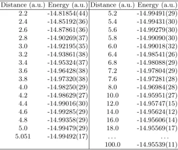
Our results for the potential energy curve of the Li2 molecule are presented in
Figure 3 (graphical form) and Table 1 (raw data and error bars). Results are given for a set of 31 inter-nuclear distances. Let us emphasize that the data are of a very high-quality and the energy curve presented is, to the best of our knowledge, the most accurate energy curve ever published. To illustrate this point, let us mention that the dissociation energy defined as De ≡ E(Req) −
E(R = ∞) is found to be here De= −0.0395(2) a.u. in excellent agreement with
the experimental result of De= −0.03928 a.u., Ref.[15]. A much more detailed
discussion of these results and additional data will be presented elsewhere[16]. For this application only 11Mb of memory per Fortran process was needed to allow the computation of the blocks. This feature is twofold. First, it allowed our jobs to be selected rapidly by the batch queuing systems as very few resources were requested. Second, as the memory requirements are very low, the code was able to run on any kind of machine. This allowed our jobs to enter both the 32-bit (x86) and 64-bit (x86 64) queues.
4.1 Grid Performance
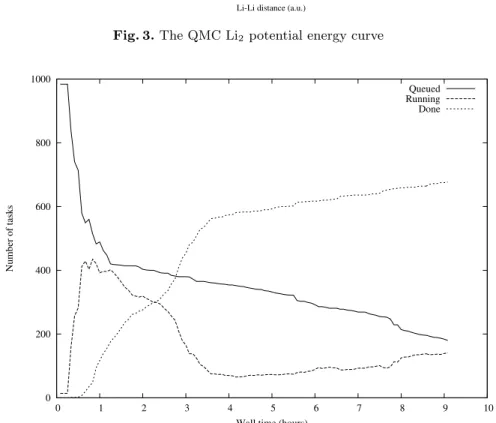
A typical analysis of the grid performance can be seen on Figure 4. Here we report the number of queued, running and executed tasks as a function of time for the submission of a parametric job of 1000 tasks.
One can see that after a very limited amount of time (less than one hour) almost half of the tasks were in a running status. Correspondingly the number of queued tasks undergoes a very rapid decay, indicating that a consistent per-centage of the submitted tasks did not spend a significant amount of time in the queue. This feature is a consequence of the very limited amount of resources requested by the job, and by the fact that virtually all the queues could be used,
-15 -14.99 -14.98 -14.97 -14.96 -14.95 -14.94 -14.93 -14.92 4 6 8 10 12 14 16 18 Energy (a.u.)
Li-Li distance (a.u.)
Fig. 3.The QMC Li2 potential energy curve
0 200 400 600 800 1000 0 1 2 3 4 5 6 7 8 9 10 Number of tasks
Wall time (hours)
Queued Running Done
Table 1. Quantum Monte Carlo energies (atomic units) as a function of the Li-Li distance (atomic units). Values in parenthesis correspond to the statistical error on the two last digits.
Distance (a.u.) Energy (a.u.) Distance (a.u.) Energy (a.u.)
2.2 -14.81854(44) 5.2 -14.99491(29) 2.4 -14.85192(36) 5.4 -14.99431(30) 2.6 -14.87861(36) 5.6 -14.99279(30) 2.8 -14.90269(37) 5.8 -14.99090(30) 3.0 -14.92195(35) 6.0 -14.99018(32) 3.2 -14.93861(38) 6.4 -14.98541(26) 3.4 -14.95324(37) 6.8 -14.98088(29) 3.6 -14.96428(38) 7.2 -14.97804(29) 3.8 -14.97320(38) 7.6 -14.97281(28) 4.0 -14.98250(29) 8.0 -14.96984(28) 4.2 -14.98629(27) 10.0 -14.95951(27) 4.4 -14.99016(30) 12.0 -14.95747(15) 4.6 -14.99285(29) 14.0 -14.95624(12) 4.8 -14.99358(29) 16.0 -14.95606(14) 5.0 -14.99479(29) 18.0 -14.95569(17) 5.051 -14.99492(17) . . . . 100.0 -14.95539(11)
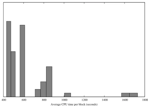
and should therefore be ascribed to the high flexibility of our approach. Corre-spondingly the number of running tasks experiences a maximum at about one hour. It is also important to notice the high asymetry of the peak, indicating that while the maximum amount of running tasks is achieved quite rapidly, the high efficiency (number of running tasks) is mantained for a considerable amount of time before a degradation. The number of completed tasks too experiences a quite rapid increase. After about four hours the numbers of running tasks re-mains constant and quite low, and consequently a small variation is observed on the number of completed tasks. The decayng of the number of running job is due to the fact that a vast majority of tasks have been completed achieving the completion of the desired number of blocks. The remaining jobs (about 50) can be abscribed to tasks running on very slow processors and so requiring a greater amount of time to complete the blocks, moreover in some cases some of the jobs could be considered as ”ghost” i.e. labelled as running although being stalled. After 9 hours the job was cancelled since the desired precision level had been achieved, even if only about 700-800 tasks were actually completed. The overall process required on average about 1000 CPU hours for each geometry equivalent to about 40 days of CPU time. It is also noteworthy to comment the distribution of the CPU time per block for each task (Figure 5), this difference reflects the fact that some tasks have been performed on slower nodes. Again this asymetry did not influence the final result since the final statistics were performed on the total amount of blocks.
400 600 800 1000 1200 1400 1600 1800 Average CPU time per block (seconds)
Fig. 5.Histogram of the CPU time per block. This figure shows the heterogeneity of
the used processors.
5
Conclusions
An efficient grid implementation of a massively parallel quantum Monte Carlo code has been presented. The strategy employed has been presented in detail. Some test applications have been performed on the EGEE-III grid architecture showing the efficiency and flexibility of our implementation. As shown, our ap-proach enables to exploit the computational power and resources of the grid for the solution of a non-trivial N -body problem of chemistry. It must be empha-sized that the very important computational gain obtained here has concerned the simulation of the Shr¨odinger equation for a single fixed nuclear geometry (single point energy calculation). This is in sharp contrast with the common situation in computational chemistry where parallelism is not used (or partially used) for solving the problem at hand (algorithms are in general poorly par-allelized) but rather for making independent simulations at different nuclear geometries (trivial parallelization based on different inputs). We believe that the quantum Monte Carlo approach which is based on Markov chain processes and on the accumulation of statistics for independent events can represent an ideal test bed for the use of grid environments in computational chemistry. Finally, we note that the combination of grid computing power and of the QMC ability to treat chemical problems at a high-level of accuracy can open the way to the possibility of studying fascinating problems (from the domain of nano-sciences
to biological systems) which are presently out of reach.
Acknowledgements
Support from the French CNRS and from University of Toulouse is gratefully acknowledged. The authors also wish to thank the French PICS action 4263 and European COST in Chemistry D37 “GridChem”. Acknowledgments are also due to the EGEE-III grid organization and to the CompChem virtual organization.
References
1. W.M.C. Foulkes, L. Mit´a˘s, R.J. Needs, G. Rajogopal: Quantum Monte Carlo
sim-ulations of solids Rev. Mod. Phys. 73, 33 (2001)
2. B.L. Hammond, W.A. Lester Jr., P.J. Reynolds: Monte Carlo Methods in Ab Initio Quantum Chemistry. World Scientific (1994)
3. http://www.eu-egee.org/
4. T.H. Dunning Jr.: Gaussian basis sets for use in correlated molecular calculations. I) The atoms boron through neon and hydrogen J. Chem. Phys. 90, 1007 (1989) 5. QMC=Chem is a general-purpose quantum Monte Carlo code for electronic
struc-ture calculations. Developped by M. Caffarel, A. Scemama and collaborators at Lab. de Chimie et Physique Quantiques, CNRS and Universit´e de Toulouse, http://qmcchem.ups-tlse.fr
6. P. L’Ecuyer: Tables of maximally equidistributed combined LFSR generators Math. of Comput. 68, 261–269 (1999)
7. W. Gropp, E. Lusk, N. Doss, A. Skjellum: A high-performance, portable implemen-tation of the MPI message passing interface standard Parallel Computing, North-Holland 22, 789–828, (1996).
8. http://www.python.org/
9. R. L. Rivest.: Technical report. Internet Activities Board, April (1992)
10. A. Scemama, A. Monari, C. Angeli, S. Borini, S. Evangelisti, E. Rossi: Common Format for Quantum Chemistry Interoperability: Q5Cost format and library O. Gervasi et al. (Eds.) Lecture Notes in Computer Science, Computational Science and Its Applications, ICCSA, Part I, LNCS 5072, 1094–1107 (2008)
11. V. Vetere, A. Monari, A. Scemama, G. L. Bendazzoli, S. Evangelisti: A Theoretical Study of Linear Beryllium Chains: Full Configuration Interaction J. Chem. Phys. 130, 024301 (2009)
12. G.L. Bendazzoli, S. Evangelisti: A vector and parallel full configuration interaction algorithm J. Chem. Phys. 98, 3141-3150 (1993)
13. L. Gagliardi, G.L. Bendazzoli, S. Evangelisti: Direct-list algorithm for configuration interaction calculations J. Comp. Chem. 18, 1329 (1997)
14. G. Karlstr¨om, R. Lindh, A. Malmqvist, B. O. Roos, U. Ryde, V. Veryazov,
P.-O. Widmark, M. Cossi, B. Schimmelpfennig, P. Neogrady, L. Seijo: MOLCAS: a program package for computational chemistry Computational Material Science 28, 222 (2003)
15. C. Filipp, C.J. Umrigar: Multiconfiguration wave functions for quantum Monte Carlo calculations of firstrow diatomic molecules J. Chem. Phys. 105, 213 (1996)
16. A. Monari, A. Scemama, M. Caffarel: A quantum Monte Carlo study of the
fixed-node Li2potential energy curve using Full Configuration Interaction nodes