HAL Id: hal-01312917
https://hal.archives-ouvertes.fr/hal-01312917
Submitted on 9 May 2016
HAL is a multi-disciplinary open access
archive for the deposit and dissemination of
sci-entific research documents, whether they are
pub-lished or not. The documents may come from
teaching and research institutions in France or
abroad, or from public or private research centers.
L’archive ouverte pluridisciplinaire HAL, est
destinée au dépôt et à la diffusion de documents
scientifiques de niveau recherche, publiés ou non,
émanant des établissements d’enseignement et de
recherche français ou étrangers, des laboratoires
publics ou privés.
A Survey of Stochastic Simulation and Optimization
Methods in Signal Processing
Marcelo Alejandro Pereyra, Philip Schniter, Emilie Chouzenoux,
Jean-Christophe Pesquet, Jean-Yves Tourneret, Alfred O. Hero, Steve
Mclaughlin
To cite this version:
Marcelo Alejandro Pereyra, Philip Schniter, Emilie Chouzenoux, Jean-Christophe Pesquet, Jean-Yves
Tourneret, et al.. A Survey of Stochastic Simulation and Optimization Methods in Signal Processing.
IEEE Journal of Selected Topics in Signal Processing, IEEE, 2015, vol. 10 (n° 2), pp. 224-241.
�10.1109/JSTSP.2015.2496908�. �hal-01312917�
O
pen
A
rchive
T
OULOUSE
A
rchive
O
uverte (
OATAO
)
OATAO is an open access repository that collects the work of Toulouse researchers and
makes it freely available over the web where possible.
This is an author-deposited version published in :
http://oatao.univ-toulouse.fr/
Eprints ID : 15732
To link to this article : DOI:10.1109/JSTSP.2015.2496908
URL :
http://dx.doi.org/10.1109/JSTSP.2015.2496908
To cite this version : Pereyra, Marcelo Alejandro and Schniter, Philip
and Chouzenoux, Emilie and Pesquet, Jean-Christophe and Tourneret,
Jean-Yves and Hero, Alfred O. and McLaughlin, Steve A Survey of
Stochastic Simulation and Optimization Methods in Signal
Processing. (2015) IEEE Journal on Selected Topics in Signal
Processing, vol. 10 (n° 2). pp. 224-241. ISSN 1932-4553
Any correspondence concerning this service should be sent to the repository
administrator:
[email protected]
A Survey of Stochastic Simulation and Optimization
Methods in Signal Processing
Marcelo Pereyra, Member, IEEE, Philip Schniter, Fellow, IEEE, Émilie Chouzenoux, Member, IEEE,
Jean-Christophe Pesquet, Fellow, IEEE, Jean-Yves Tourneret, Senior Member, IEEE,
Alfred O. Hero, III, Fellow, IEEE, and Steve McLaughlin, Fellow, IEEE
Abstract—Modern signal processing (SP) methods rely very
heavily on probability and statistics to solve challenging SP problems. SP methods are now expected to deal with ever more complex models, requiring ever more sophisticated computa-tional inference techniques. This has driven the development of statistical SP methods based on stochastic simulation and optimization. Stochastic simulation and optimization algorithms are computationally intensive tools for performing statistical inference in models that are analytically intractable and beyond the scope of deterministic inference methods. They have been recently successfully applied to many difficult problems involving complex statistical models and sophisticated (often Bayesian) statistical inference techniques. This survey paper offers an in-troduction to stochastic simulation and optimization methods in signal and image processing. The paper addresses a variety of high-dimensional Markov chain Monte Carlo (MCMC) methods as well as deterministic surrogate methods, such as variational Bayes, the Bethe approach, belief and expectation propagation and approximate message passing algorithms. It also discusses a range of optimization methods that have been adopted to solve sto-chastic problems, as well as stosto-chastic methods for deterministic optimization. Subsequently, areas of overlap between simulation
Manuscript received April 30, 2015; revised August 29, 2015; accepted Oc-tober 09, 2015. Date of publication November 02, 2015; date of current version February 11, 2016. This work was supported in part by the SuSTaIN program under EPSRC Grant EP/D063485/1 at the Department of Mathematics, Uni-versity of Bristol., in part by the CNRS Imag’in project under Grant 2015OPTI-MISME, in part by the HYPANEMA ANR Project under Grant ANR-12-BS03-003, in part by the BNPSI ANR Project ANR-13- BS-03-0006-01, and in part by the project L ABX-0040-CIMI as part of the program ANR-11-IDEX-0002-02 within the thematic trimester on image processing. The work of S. McLaughlin was supported by the EPSRC under Grant EP/J015180/1. The work of M. Pereyra was supported by a Marie Curie Intra-European Fellow-ship for Career Development. The work of P. Schniter was supported by the National Science Foundation under Grants CCF-1218754 and CCF-1018368. The work of A. Hero was supported by the Army Research Office under Grant W911NF-15-1-0479. The Editor-in-Chief coordinating the review of this man-uscript and approving it for publication was Dr. Fernando Pereira.
M. Pereyra is with the School of Mathematics, University of Bristol, Bristol BS8 1TW, U.K. (e-mail: [email protected]).
P. Schniter is with the Department of Electrical and Computer Engineering, The Ohio State University, Columbus, OH 43210 USA (e-mail: schniter@ece. osu.edu).
É. Chouzenoux and J.-C. Pesquet are with the Laboratoire d’Informatique Gaspard Monge, Université Paris-Est, 77454 Marne la Vallée, France (e-mail: [email protected]; [email protected]).
J.-Y. Tourneret is with the INP-ENSEEIHT-IRIT-TeSA, University of Toulouse, 31071 Toulouse, France (e-mail: [email protected]).
A. O. Hero III is with the Department of Electrical Engineering and Computer Science, University of Michigan, Ann Arbor, MI 48109-2122 USA (e-mail: [email protected]).
S. McLaughlin is with Engineering and Physical Sciences, Heriot Watt Uni-versity, Edinburgh EH14 4AS, U.K. (e-mail: [email protected]).
Digital Object Identifier 10.1109/JSTSP.2015.2496908
and optimization, in particular optimization-within-MCMC and MCMC-driven optimization are discussed.
Index Terms—Bayesian inference, Markov chain Monte Carlo,
proximal optimization algorithms, variational algorithms for ap-proximate inference.
I. INTRODUCTION
M
ODERN signal processing (SP) methods, (we use SP here to cover all relevant signal and image processing problems), rely very heavily on probabilistic and statistical tools; for example, they use stochastic models to represent the data observation process and the prior knowledge available, and they obtain solutions by performing statistical inference (e.g., using maximum likelihood or Bayesian strategies). Sta-tistical SP methods are, in particular, routinely applied to many and varied tasks and signal modalities, ranging from resolu-tion enhancement of medical images to hyperspectral image unmixing; from user rating prediction to change detection in social networks; and from source separation in music analysis to speech recognition.However, the expectations and demands on the performance of such methods are constantly rising. SP methods are now expected to deal with challenging problems that require ever more complex models, and more importantly, ever more so-phisticated computational inference techniques. This has driven the development of computationally intensive SP methods based on stochastic simulation and optimization. Stochastic simulation and optimization algorithms are computationally intensive tools for performing statistical inference in models that are analytically intractable and beyond the scope of deterministic inference methods. They have been recently successfully applied to many difficult SP problems involving complex statistical models and sophisticated (often Bayesian) statistical inference analyses. These problems can generally be formulated as inverse problems involving partially unknown observation processes and imprecise prior knowledge, for which they delivered accurate and insightful results. These stochastic algorithms are also closely related to the random-ized, variational Bayes and message passing algorithms that are pushing forward the state of the art in approximate statis-tical inference for very large-scale problems. The key thread that makes stochastic simulation and optimization methods appropriate for these applications is the complexity and high dimensionality involved. For example in the case of hyper-spectral imaging the data being processed can involve images
of 2048 by 1024 pixels across up to hundreds or thousands of wavelengths.
This survey paper offers an introduction to stochastic simula-tion and optimizasimula-tion methods in signal and image processing. The paper addresses a variety of high-dimensional Markov chain Monte Carlo (MCMC) methods as well as determin-istic surrogate methods, such as variational Bayes, the Bethe approach, belief and expectation propagation and approxi-mate message passing algorithms. It also discusses a range of stochastic optimization approaches. Subsequently, areas of overlap between simulation and optimization, in particular optimization-within-MCMC and MCMC-driven optimization are discussed. Some methods such as sequential Monte Carlo methods or methods based on importance sampling are not considered in this survey mainly due to space limitations.
This paper seeks to provide a survey of a variety of the algo-rithmic approaches in a tutorial fashion, as well as to highlight the state of the art, relationships between the methods, and po-tential future directions of research. In order to set the scene and inform our notation, consider an unknown random vector of interest and an observed data vector , related to by a statistical model with like-lihood function potentially parametrized by a deter-ministic vector of parameters . Following a Bayesian inference approach, we model our prior knowledge about with a prior distribution , and our knowledge about after observing
with the posterior distribution
(1) where the normalizing constant
(2) is known as the “evidence”, model likelihood, or the partition function. Although the integral in (2) suggests that all are continuous random variables, we allow any random variable to be either continuous or discrete, and replace the integral with a sum as required.
In many applications, we would like to evaluate the posterior or some summary of it, for instance point estimates of such as the conditional mean (i.e., MMSE estimate)
, uncertainty reports such as the conditional variance
, or expected log statistics as used in the expectation maxi-mization (EM) algorithm [1]–[3]
(3) where the expectation is taken with respect to . How-ever, when the signal dimensionality is large, the integral in (2), as well as those used in the posterior summaries, are often computationally intractable. Hence, the interest in compu-tationally efficient alternatives. An alternative that has received a lot of attention in the statistical SP community is maximum-a-posteriori (MAP) estimation. Unlike other posterior summaries, MAP estimates can be computed by finding the value of max-imizing , which for many models is significantly more computationally tractable than numerical integration. In the se-quel, we will suppress the dependence on in the notation, since it is not of primary concern.
The paper is organized as follows. After this brief intro-duction where we have introduced the basic notation adopted, Section II discusses stochastic simulation methods, and in particular a variety of MCMC methods. In Section III we discuss deterministic surrogate methods, such as variational Bayes, the Bethe approach, belief and expectation propagation, and provide a brief summary of approximate message passing algorithms. Section IV discusses a range of optimization methods for solving stochastic problems, as well as stochastic methods for solving deterministic optimization problems. Sub-sequently, in Section V we discuss areas of overlap between simulation and optimization, in particular the use of optimiza-tion techniques within MCMC algorithms and MCMC-driven optimization, and suggest some interesting areas worthy of exploration. Finally, in Section VI we draw together thoughts, observations and conclusions.
II. STOCHASTICSIMULATIONMETHODS
Stochastic simulation methods are sophisticated random number generators that allow samples to be drawn from a user-specified target density , such as the posterior . These samples can then be used, for example, to approximate probabilities and expectations by Monte Carlo integration [4, Ch. 3]. In this section we will focus on MCMC methods, an important class of stochastic simulation techniques that operate by constructing a Markov chain with stationary distribution . In particular, we concentrate on Metropolis-Hastings (MH) algorithms for high-dimensional models (see [5] for a more general recent review of MCMC methods). It is worth empha-sizing, however, that we do not discuss many other important approaches to simulation that also arise often in signal pro-cessing applications, such as “particle filters” or sequential Monte Carlo methods [6], [7], and approximate Bayesian computation [8].
A cornerstone of MCMC methodology is the MH algorithm [4, Ch. 7], [9], [10], a universal machine for constructing Markov chains with stationary density . Given some generic proposal distribution , the generic MH algorithm proceeds as follows.
Algorithm 1 Metropolis-Hastings algorithm (generic version)
Set an initial state
for to do
Generate a candidate state from a proposal Compute the acceptance probability
Generate
if then
Accept the candidate and set
else
Reject the candidate and set
end if end for
Under mild conditions on , the chains generated by Algo. 1 are ergodic and converge to the stationary distribution [11], [12]. An important feature of this algorithm is that computing the acceptance probabilities does not require knowledge of the normalization constant of (which is often not available in Bayesian inference problems). The intuition for the MH algo-rithm is that the algoalgo-rithm proposes a stochastic perturbation to the state of the chain and applies a carefully defined decision rule to decide if this perturbation should be accepted or not. This decision rule, given by the random accept-reject step in Algo. 1, ensures that at equilibrium the samples of the Markov chain have as marginal distribution.
The specific choice of will of course determine the effi-ciency and the convergence properties of the algorithm. Ideally one should choose to obtain a perfect sampler (i.e., with candidates accepted with probability 1); this is of course not practically feasible since the objective is to avoid the complexity of directly simulating from . In the remainder of this section we review strategies for specifying for high-dimensional models, and discuss relative advantages and disadvantages. In order to compare and optimize the choice of , a performance criterion needs to be chosen. A natural criterion is the stationary inte-grated autocorrelation time for some relevant scalar summary statistic , i.e.,
(4) with , and where denotes the correlation op-erator. This criterion is directly related to the effective number of independent Monte Carlo samples produced by the MH algo-rithm, and therefore to the mean squared error of the resulting Monte Carlo estimates. Unfortunately drawing conclusions di-rectly from (4) is generally not possible because is highly de-pendent on the choice of , with different choices often leading to contradictory results. Instead, MH algorithms are generally studied asymptotically in the infinite-dimensional model limit. More precisely, in the limit , the algorithms can be studied using diffusion process theory, where the dependence on vanishes and all measures of efficiency become proportional to the diffusion speed. The “complexity” of the algorithms can then be defined as the rate at which efficiency deteriorates as
, e.g., (see [13] for an introduction to this topic and details about the relationship between the efficiency of MH algorithms and their average acceptance probabilities or accep-tance rates)1.
Finally, it is worth mentioning that despite the generality of this approach, there are some specific models for which conven-tional MH sampling is not possible because the computation of is intractable (e.g., when involves an intractable function of , such as the partition function of the Potts-Markov random field). This issue has received a lot of attention in the recent MCMC literature, and there are now several variations of the MH construction for intractable models [8], [14]–[16].
1Notice that this measure of complexity of MCMC algorithms does not take
into account the computational costs related to generating candidate states and evaluating their Metropolis-Hastings acceptance probabilities, which typically also scale at least linearly with the problem dimension .
A. Random Walk Metropolis-Hastings Algorithms
The so-called random walk Metropolis-Hastings (RWMH) algorithm is based on proposals of the form
, where typically for some positive-definite co-variance matrix [4, Ch. 7.5]. This algorithm is one of the most widely used MCMC methods, perhaps because it has very ro-bust convergence properties and a relatively low computational cost per iteration. It can be shown that the RWMH algorithm is geometrically ergodic under mild conditions on [17]. Geo-metric ergodicity is important because it guarantees a central limit theorem for the chains, and therefore that the samples can be used for Monte Carlo integration. However, the myopic na-ture of the random walk proposal means that the algorithm often requires a large number of iterations to explore the parameter space, and will tend to generate samples that are highly corre-lated, particularly if the dimension is large (the performance of this algorithm generally deteriorates at rate , which is worse than other more advanced stochastic simulation MH al-gorithms [18]). This drawback can be partially mitigated by ad-justing the matrix to approximate the covariance structure of , and some adaptive versions of RWHM perform this adapta-tion automatically. For sufficiently smooth target densities, per-formance is further optimized by scaling to achieve an accep-tance probability of approximately 20% – 25% [18].
B. Metropolis Adjusted Langevin Algorithms
The Metropolis adjusted Langevin algorithm (MALA) is an advanced MH algorithm inspired by the Langevin diffusion process on , defined as the solution to the stochastic differ-ential equation [19]
(5) where is the Brownian motion process on and
denotes some initial condition. Under appropriate stability con-ditions, converges in distribution to as , and is therefore potentially interesting for drawing samples from . Since direct simulation from is only possible in very spe-cific cases, we consider a discrete-time forward Euler approxi-mation to (5) given by
(6) where the parameter controls the discrete-time increment. Under certain conditions on and , (6) produces a good approximation of and converges to a stationary density which is close to . In MALA this approximation error is corrected by introducing an MH accept-reject step that guaran-tees convergence to the correct target density . The resulting algorithm is equivalent to Algo. 1 above, with proposal
(7) By analyzing the proposal (7) we notice that, in addition to the Langevin interpretation, MALA can also be interpreted as an MH algorithm that, at each iteration , draws a candidate from
a local quadratic approximation to around , with as an approximation to the Hessian matrix.
In addition, the MALA proposal can also be defined using a matrix-valued time step . This modification is related to redefining (6) in an Euclidean space with the inner product [20]. Again, the matrix should capture the cor-relation structure of to improve efficiency. For example, can be the spectrally-positive version of the inverse Hessian matrix of [21], or the inverse Fisher information matrix of the statistical observation model [20]. Note that, in a similar fashion to preconditioning in optimization, using the exact full Hessian or Fisher information matrix is often too computation-ally expensive in high-dimensional settings and more efficient representations must be used instead. Alternatively, adaptive versions of MALA can learn a representation of the covariance structure online [22]. For sufficiently smooth target densities, MALA’s performance can be further optimized by scaling (or ) to achieve an acceptance probability of approximately 50% – 60% [23].
Finally, there has been significant empirical evidence that MALA can be very efficient for some models, particularly in high-dimensional settings and when the cost of computing the gradient is low. Theoretically, for sufficiently smooth , the complexity of MALA scales at rate
[23], comparing very favorably to the rate of RWMH algorithms. However, the convergence properties of the con-ventional MALA are not as robust as those of the RWMH algorithm. In particular, MALA may fail to converge if the tails of are super-Gaussian or heavy-tailed, or if is chosen too large [19]. Similarly, MALA might also perform poorly if is not sufficiently smooth, or multi-modal. Improving MALA’s convergence properties is an active research topic. Many limitations of the original MALA algorithm can now be avoided by using more advanced versions [20], [24]–[27].
C. Hamiltonian Monte Carlo
The Hamiltonian Monte Carlo (HMC) method is a very el-egant and successful instance of an MH algorithm based on auxiliary variables [28]. Let , positive definite, and consider the augmented target density
, which admits the desired target density as marginal. The HMC method is based on the observation that the trajectories defined by the so-called
Hamil-tonian dynamics preserve the level sets of . A point that evolves according to the set of differential equations (8) during some simulation time period
(8) yields a point that verifies . In MCMC terms, the deterministic proposal (8) has as in-variant distribution. Exploiting this property for stochastic sim-ulation, the HMC algorithm combines (8) with a stochastic sam-pling step, , that also has invariant distribution , and that will produce an ergodic chain. Finally, as with the Langevin diffusion (5), it is generally not possible to solve
the Hamiltonian (8) exactly. Instead, we use a leap-frog approx-imation detailed in [28]
(9) where again the parameter controls the discrete-time incre-ment. The approximation error introduced by (9) is then cor-rected with an MH step targeting . This algorithm is summarized in Algo. 2 below (see [28] for details about the derivation of the acceptance probability).
Algorithm 2 Hamiltonian Monte Carlo (with leap-frog)
Set an initial state , , and .
for to do
Refresh the auxiliary variable .
Generate a candidate by propagating the current state with leap-frog steps of length defined in (9).
Compute the acceptance probability
Generate .
if then
Accept the candidate and set .
else
Reject the candidate and set .
end if end for
Note that to obtain samples from the marginal it is suf-ficient to project the augmented samples onto the original space of (i.e., by discarding the auxiliary variables ). It is also worth mentioning that under some regularity condition on , the leap-frog approximation (9) is time-re-versible and volume-preserving, and that these properties are key to the validity of the HMC algorithm [28].
Finally, there has been a large body of empirical evidence supporting HMC, particularly for high-dimensional models. Unfortunately, its theoretical convergence properties are much less well understood [29]. It has been recently established that for certain target densities the complexity of HMC scales at rate
, comparing favorably with MALA’s rate
[30]. However, it has also been observed that, as with MALA, HMC may fail to converge if the tails of are super-Gaussian or heavy-tailed, or if is chosen too large. HMC may also perform poorly if is multi-modal, or not sufficiently smooth.
Of course, the practical performance of HMC also depends strongly on the algorithm parameters , and [29]. The co-variance matrix should be designed to model the correlation structure of , which can be determined by performing pilot runs, or alternatively by using the strategies described in [20], [21], [31]. The parameters and should be adjusted to obtain
an average acceptance probability of approximately 60% – 70% [30]. Again, this can be achieved by performing pilot runs, or by using an adaptive HMC algorithm that adjusts these parameters automatically [32], [33].
D. Gibbs Sampling
The Gibbs sampler (GS) is another very widely used MH al-gorithm which operates by updating the elements of individ-ually, or by groups, using the appropriate conditional distribu-tions [4, Ch. 10]. This divide-and-conquer strategy often leads to important efficiency gains, particularly if the conditional den-sities involved are “simple”, in the sense that it is computation-ally straightforward to draw samples from them. For illustra-tion, suppose that we split the elements of in three groups , and that by doing so we obtain three con-ditional densities , , and
that are “simple” to sample. Using this decomposition, the GS targeting proceeds as in Algo. 3. The Markov kernel resulting from concatenating the component-wise kernels admits as joint invariant distribution, and thus the chain produced by Algo. 3 has the desired target density (see [4, Ch. 10] for a review of the theory behind this algorithm). This fundamental property holds even if the simulation from the conditionals is done by using other MCMC algorithms (e.g., RWMH, MALA or HMC steps targeting the conditional densities), though this may result in a deterioration of the algorithm convergence rate. Similarly, the property also holds if the frequency and order of the updates is scheduled randomly and adaptively to improve the overall performance.
Algorithm 3 Gibbs sampler algorithm
Set an initial state
for to do
Generate Generate Generate
end for
As with other MH algorithms, the performance of the GS de-pends on the correlation structure of . Efficient samplers seek to update simultaneously the elements of that are highly cor-related with each other, and to update “slow-moving” elements more frequently. The structure of can be determined by pilot runs, or alternatively by using an adaptive GS that learns it on-line and that adapts the updating schedule accordingly as de-scribed in [34]. However, updating elements in parallel often involves simulating from more complicated conditional distri-butions, and thus introduces a computational overhead. Finally, it is worth noting that the GS is very useful for SP models, which typically have sparse conditional independence structures (e.g., Markovian properties) and conjugate priors and hyper-priors from the exponential family. This often leads to simple one-di-mensional conditional distributions that can be updated in par-allel by groups [16], [35].
E. Partially Collapsed Gibbs Sampling
The partially collapsed Gibbs sampler (PCGS) is a recent de-velopment in MCMC theory that seeks to address some of the limitations of the conventional GS [36]. As mentioned previ-ously, the GS performs poorly if strongly correlated elements of are updated separately, as this leads to chains that are highly correlated and to an inefficient exploration of the parameter space. However, updating several elements together can also be computationally expensive, particularly if it requires simulating from difficult conditional distributions. In collapsed samplers, this drawback is addressed by carefully replacing one or sev-eral conditional densities by partially collapsed, or marginal-ized conditional distributions.
For illustration, suppose that in our previous example the sub-vectors and exhibit strong dependencies, and that as a result the GS of Algo. 3 performs poorly. Assume that we are able to draw samples from the marginalized conditional density , which does not depend on . This leads to the PCGS described in Algo. 4 to sample from , which “partially collapses” Algo. 3 by replacing
with .
Algorithm 4 Partially collapsed Gibbs sampler
Set an initial state
for to do
Generate Generate Generate
end for
Van Dyk and Park [36] established that the PCGS is always at least as efficient as the conventional GS, and it has been ob-served that the PCGS is remarkably efficient for some statistical models [37], [38]. Unfortunately, PCGSs are not as widely ap-plicable as GSs because they require simulating exactly from the partially collapsed conditional distributions. In general, using MCMC simulation (e.g., MH steps) within a PCGS will lead to an incorrect MCMC algorithm [39]. Similarly, altering the order of the updates (e.g., by permuting the simulations of and in Algo. 4) may also alter the target density [36].
III. SURROGATES FORSTOCHASTICSIMULATION
A. Variational Bayes
In the variational Bayes (VB) approach described in [40], [41], the true posterior is approximated by a density , where is a subset of valid densities on . In particular,
(10) where denotes the Kullback-Leibler (KL) divergence between and . As a result of the optimization in (10) over a function, this is termed “variational Bayes” because of the re-lation to the calculus of variations [42]. Recalling that
we see that when includes all valid densi-ties on . However, the premise is that is too difficult to work with, and so is chosen as a balance between fidelity and tractability.
Note that the use of , rather than , implies a search for a that agrees with the true posterior over the set of where is large. We will revisit this choice when discussing expectation propagation in Section III-E.
Rather than working with the KL divergence directly, it is common to decompose it as follows
(11) where
(12) is known as the Gibbs free energy or variational free energy. Rearranging (11), we see that
(13) as a consequence of . Thus, can be interpreted as an upper bound on the negative log partition. Also, because is invariant to , the optimization (10) can be rewritten as
(14) which avoids the difficult integral in (2). In the sequel, we will discuss several strategies to solve the variational optimization problem (14).
B. The Mean-Field Approximation
A common choice of is the set of fully factorizable densi-ties, resulting in the mean-field approximation [44], [45]
(15) Substituting (15) into (12) yields the mean-field free energy
(16)
where denotes the
differen-tial entropy. Furthermore, for , (16) can be written as
(17) (18)
where for .
Equation (17) implies the optimality condition
(19)
where and where is defined
as in (18) but with in place of . Equation (19) suggests an iterative coordinate-ascent algorithm: update each component of while holding the others fixed. But this requires solving the integral in (18). A solution arises when the conditionals belong to the same exponential family of distributions [46], i.e.,
(20) where the sufficient statistic parameterizes the family. The exponential family encompasses a broad range of distribu-tions, notably jointly Gaussian and multinomial . Plug-ging and (20) into (18) imme-diately gives
(21) where the expectation is taken over . Thus, if each is chosen from the same family, i.e., , then (19) reduces to the moment-matching condition
(22) where is the optimal value of .
C. The Bethe Approach
In many cases, the fully factored model (15) yields too gross of an approximation. As an alternative, one might try to fit a model that has a similar dependency structure as . In the sequel, we assume that the true posterior factors as
(23) where are subvectors of (sometimes called cliques or
outer clusters) and are non-negative potential functions. Note that the factorization (23) defines a Gibbs random field when . When a collection of variables always appears together in a factor, we can collect them into , an
inner cluster, although it is not necessary to do so. For
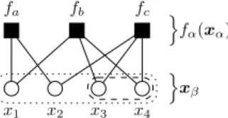
sim-plicity we will assume that these are non-overlapping (i.e., ), so that represents a partition of . The factorization (23) can then be drawn as a factor graph to help visualize the structure of the posterior, as in Fig. 1.
We now seek a tractable way to build an approximation with the same dependency structure as (23). But rather than designing as a whole, we design the cluster marginals, and , which must be non-negative, normal-ized, and consistent
(24) (25) (26) where gathers the components of that are contained in the cluster and not in the cluster , and denotes the
neigh-Fig. 1. An example of a factor graph, which is a bipartite graph consisting of variable nodes, (circles/ovals), and factor nodes, (boxes). In this example, , , . There are several choices for the inner clusters . One is the full factorization ,
, , and . Another is the partial factorization , , and , which results in the “super node” in the dashed oval. Another is no factorization: , resulting in the “super node” in the dotted oval. In the latter case, we redefine each factor to have the full domain (with trivial dependencies where needed).
borhood of the factor ( i.e., the set of inner clusters con-nected to ).
In general, it is difficult to specify from its cluster marginals. However, in the special case that the factor graph has a tree structure (i.e., there is at most one path from one node in the graph to another), we have [47]
(27) where is the neighborhood size of the cluster . In this case, the free energy (12) simplifies to
(28)
where is known as the Bethe free energy (BFE) [47]. Clearly, if the true posterior has a tree structure, and no constraints beyond (24)–(26) are placed on the cluster marginals , then minimization of will recover the cluster marginals of the true posterior. But even when is not a tree, can be used as an approximation of the Gibbs free energy , and minimizing can be inter-preted as designing a that locally matches the true posterior.
The remaining question is how to efficiently minimize subject to the (linear) constraints (24)–(26). Complicating matters is the fact that is the sum of convex KL divergences and concave entropies. One option is direct minimization using a “double loop” approach like the concave-convex procedure (CCCP) [48], where the outer loop linearizes the concave term about the current estimate and the inner loop solves the resulting convex optimization problem (typically with an iterative technique). Another option is belief propagation, which is described below.
D. Belief Propagation
Belief propagation (BP) [49], [50] is an algorithm for com-puting (or approximating) marginal probability density func-tions (pdfs)2like and by propagating messages
on a factor graph. The standard form of BP is given by the
2Note that another form of BP exists to compute the maximum a posteriori
(MAP) estimate known as the “max-product” or “min-sum” algorithm [50]. However, this approach does not address the problem of com-puting surrogates for stochastic methods, and so is not discussed further.
sum-product algorithm (SPA) [51], which computes the fol-lowing messages from each factor node to each variable (super) node and vice versa
(29) (30) These messages are then used to compute the beliefs
(31) (32) which must be normalized in accordance with (25). The mes-sages (29)-(30) do not need to be normalized, although it is often done in practice to prevent numerical overflow.
When the factor graph has a tree structure, the BP-com-puted marginals coincide with the true marginals after one round of forward and backward message passes. Thus, BP on a tree-graph is sometimes referred to as the forward-backward algo-rithm, particularly in the context of hidden Markov models [52]. In the tree case, BP is akin to a dynamic programming algorithm that organizes the computations needed for marginal evaluation in a tractable manner.
When the factor graph has cycles or “loops,” BP can still be applied by iterating the message computations (29)-(30) until convergence (not guaranteed), which is known as loopy
BP (LBP). However, the corresponding beliefs (31)-(32) are in
general only approximations of the true marginals. This sub-optimality is expected because exact marginal computation on a loopy graph is an NP-hard problem [53]. Still, the answers computed by LBP are in many cases very accurate [54]. For ex-ample, LBP methods have been successfully applied to commu-nication and SP problems such as: turbo decoding [55], LDPC decoding [49], [56], inference on Markov random fields [57], multiuser detection [58], and compressive sensing [59], [60].
Although the excellent performance of LBP was at first a mystery, it was later established that LBP minimizes the con-strained BFE. More precisely, the fixed points of LBP coincide with the stationary points of from (28) under the constraints (24)-(26) [47]. The link between LBP and BFE can be established through the Lagrangian formalism, which converts constrained BFE minimization to an unconstrained minimization through the incorporation of additional variables known as Lagrange multipliers [61]. By setting the derivatives of the Lagrangian to zero, one obtains a set of equations that are equivalent to the message updates (29)-(30) [47]. In particular, the stationary-point versions of the Lagrange multipliers equal the fixed-point versions of the loopy SPA log-messages.
Note that, unlike the mean-field approach (15), the cluster-based nature of LBP does not facilitate an explicit description of the joint-posterior approximation from (10). The reason is that, when the factor graph is loopy, there is no straightforward relationship between the joint posterior and the cluster marginals , as explained
before (27). Instead, it is better to interpret LBP as an efficient implementation of the Bethe approach from Section III-C, which aims for a local approximation of the true posterior.
In summary, by constructing a factor graph with low-dimen-sional and applying BP or LBP, we trade the high-dimen-sional integral for a sequence of low-dimensional message computations (29)-(30). But (29)-(30) are themselves tractable only for a few families of . Typically, are limited to members of the exponential family closed under marginalization (see [62]), so that the updates of the mes-sage pdfs (29)-(30) reduce to updates of the natural parameters (i.e., in (20)). The two most common instances are multi-variate Gaussian pdfs and multinomial probability mass func-tions (pmfs). For both of these cases, when LBP converges, it tends to be much faster than double-loop algorithms like CCCP (see, e.g., [63]). However, LBP does not always converge [54].
E. Expectation Propagation
Expectation propagation (EP) [64] (see also the overviews
[62], [65]) is an iterative method of approximate inference that is reminiscent of LBP but has much more flexibility with regards to the modeling distributions. In EP, the true posterior , which is assumed to factorize as in (23), is approximated by
such that
(33) where are the same as in (23) and are referred to as “site approximations.” Although no constraints are imposed on the true-posterior factors , the approximation is restricted to a factorized exponential family. In particular,
(34) (35) with some given base measure. We note that our description of EP applies to arbitrary partitions , from the trivial partition
to the full partition .
The EP algorithm iterates the following updates over all fac-tors until convergence (not guaranteed)
(36) (37) (38) (39) (40) (41) where in (38) refers to the set of obeying (34)-(35). Es-sentially, (36) removes the th site approximation from the posterior model , and (37) replaces it with the true factor . Here, is known as the “cavity” distribution. The quantity is then projected onto the exponential family in (38). The site approximation is then updated in (39), and the old quantities
are overwritten in (40)-(41). Note that the right side of (39) de-pends only on because and differ only over . Note also that the KL divergence in (38) is reversed relative to (10).
The EP updates (37)–(41) can be simplified by leveraging the factorized exponential family structure in (34)-(35). First, for (33) to be consistent with (34)-(35), each site approximation must factor into exponential-family terms, i.e.,
(42) (43) It can then be shown [62] that (36)–(38) reduce to
(44) for all , which can be interpreted as the moment matching condition . Further-more, (39) reduces to
(45) for all . Finally, (40) and (41) reduce to and
, respectively, for all .
Interestingly, in the case that the true factors are mem-bers of an exponential family closed under marginalization, the version of EP described above is equivalent to the SPA up to a change in message schedule. In particular, for each given factor node , the SPA updates the outgoing message towards one vari-able node per iteration, whereas EP simultaneously updates the outgoing messages in all directions, resulting in (see, e.g., [41]). By restricting the optimization in (39) to a single factor , EP can be made equivalent to the SPA. On the other hand, for generic factors , EP can be viewed as a tractable approximation of the (intractable) SPA.
Although the above form of EP iterates serially through the factor nodes , it is also possible to perform the updates in par-allel, resulting in what is known as the expectation consistent (EC) approximation algorithm [66].
EP and EC have an interesting BFE interpretation. Whereas the fixed points of LBP coincide with the stationary points of the BFE (28) subject to (24)-(25) and strong consistency (26), the fixed points of EP and EC coincide with the stationary points of the BFE (28) subject to (24)-(25) and the weak consistency (i.e., moment-matching) constraint [67]
(46) EP, like LBP, is not guaranteed to converge. Hence, provably convergence double-loop algorithms have been proposed that directly minimize the weakly constrained BFE, e.g., [67].
F. Approximate Message Passing
So-called approximate message passing (AMP) algorithms [59], [60] have recently been developed for the separable gen-eralized linear model
where the prior is fully factorizable, as is the con-ditional pdf relating the observation vector to the (hidden) transform output vector , where is a known linear transform. Like EP, AMP allows tractable inference under generic3 and
.
AMP can be derived as an approximation of LBP on the factor graph constructed with inner clusters for
, with outer clusters for
and for , and with factors
. (48) In the large-system limit (LSL), i.e., for fixed ratio
, the LBP beliefs simplify to
(49) where and are iteratively updated parameters. Simi-larly, for , the belief on , denoted by , simplifies to
(50) where and are iteratively updated parameters. Each AMP iteration requires only one evaluation of the mean and variance of (49)–(50), one multiplication by and , and relatively few iterations, making it very computationally efficient, especially when these multiplications have fast im-plementations (e.g., using fast Fourier transforms and discrete wavelet transforms ).
In the LSL under i.i.d sub-Gaussian , AMP is fully char-acterized by a scalar state evolution (SE). When this SE has a unique fixed point, the marginal posterior approximations (49)–(50) are known to be exact [68], [69].
For generic , AMP’s fixed points coincide with the sta-tionary points of an LSL version of the BFE [70], [71]. When AMP converges, its posterior approximations are often very ac-curate (e.g., [72]), but AMP does not always converge. In the special case of Gaussian likelihood and prior , AMP con-vergence is fully understood: concon-vergence depends on the ratio of peak-to-average squared singular values of , and conver-gence can be guaranteed for any with appropriate damping [73]. For generic and , damping greatly helps convergence [74] but theoretical guarantees are lacking. A double-loop algo-rithm to directly minimize the LSL-BFE was recently proposed and shown to have global convergence for strictly log-concave
and under generic [75].
IV. OPTIMIZATIONMETHODS
A. Optimization Problem
The Monte Carlo methods described in Section II provide a general approach for estimating reliably posterior probabilities and expectations. However, their high computational cost often makes them unattractive for applications involving very high di-mensionality or tight computing time constraints. One alterna-tive strategy is to perform inference approximately by using
de-3More precisely, the AMP algorithm [59] handles Gaussian while the
generalized AMP (GAMP) algorithm [60] handles arbitrary .
terministic surrogates as described in Section III. Unfortunately, these faster inference methods are not as generally applicable, and because they rely on approximations, the resulting infer-ences can suffer from estimation bias. As already mentioned, if one focuses on the MAP estimator, efficient optimization tech-niques can be employed, which are often more computationally tractable than MCMC methods and, for which strong guarantees of convergence exist. In many SP applications, the computation of the MAP estimator of can be formulated as an optimization problem having the following form
(51)
where , ,
, and with . For example, may be a linear operator modeling a degradation of the signal of interest, a vector of observed data, a least-squares cri-terion corresponding to the negative log-likelihood associated with an additive zero-mean white Gaussian noise, a sparsity promoting measure, e.g., an norm, and a frame analysis transform or a gradient operator.
Often, is an additively separable function, i.e.,
(52) where . Under this condition, the previous optimization problem becomes an instance of the more general stochastic one
(53) involving the expectation
(54) where , , and are now assumed to be random variables and the expectation is computed with respect to the joint distribu-tion of , with the -th line of . More precisely, when (52) holds, (51) is then a special case of (53) with uni-formly distributed over and deterministic. Conversely, it is also possible to consider that is deterministic and that for every , , and
are identically distributed random variables. In this second sce-nario, because of the separability condition (52), the optimiza-tion problem (51) can be regarded as a proxy for (53), where the expectation is approximated by a sample estimate (or sto-chastic approximation under suitable mixing assumptions). All these remarks illustrate the existing connections between prob-lems (51) and (53).
Note that the stochastic optimization problem defined in (53) has been extensively investigated in two communities: machine learning, and adaptive filtering, often under quite different prac-tical assumptions on the forms of the functions and . In machine learning [76]–[78], indeed represents the vector of parameters of a classifier which has to be learnt, whereas in adaptive filtering [79], [80], it is generally the impulse response of an unknown filter which needs to be identified and possibly tracked. In order to simplify our presentation, in the rest of this
section, we will assume that the functions are convex and Lipschitz-differentiable with respect to their first argument (for example, they may be logistic functions).
B. Optimization Algorithms for Solving Stochastic Problems
The main difficulty arising in the resolution of the stochastic optimization problem (53) is that the integral involved in the ex-pectation term often cannot be computed in practice since it is generally high-dimensional and the underlying probability mea-sure is usually unknown. Two main computational approaches have been proposed in the literature to overcome this issue. The first idea is to approximate the expected loss function by using a finite set of observations and to minimize the associated empir-ical loss (51). The resulting deterministic optimization problem can then be solved by using either deterministic or stochastic algorithms, the latter being the topic of Section IV-C. Here, we focus on the second family of methods grounded in sto-chastic approximation techniques to handle the expectation in (54). More precisely, a sequence of identically distributed sam-ples is drawn, which are processed sequentially ac-cording to some update rule. The iterative algorithm aims to produce a sequence of random iterates converging to a solution to (53).
We begin with a group of online learning algorithms based on extensions of the well-known stochastic gradient descent (SGD) approach. Then we will turn our attention to stochastic optimization techniques developed in the context of adaptive filtering.
1) Online Learning Methods Based on SGD: Let us assume
that an estimate of the gradient of at is avail-able at each iteration . A popular strategy for solving (53) in this context leverages the gradient estimates to derive a so-called stochastic forward-backward (SFB) scheme, (also sometimes called stochastic proximal gradient algorithm)
(55) where is a sequence of positive stepsize values and is a sequence of relaxation parameters in . Here-above, denotes the proximity operator at of a lower-semicontinuous convex function
with nonempty domain, i.e., the unique minimizer of (see [81] and the references therein), and . A convergence analysis of the SFB scheme has been conducted in [82]–[85], under various assumptions on the functions , , on the stepsize sequence, and on the statistical properties of . For example, if is set to a given (deterministic) value, the sequence generated by (55) is guaranteed to converge almost surely to a solution of Problem (53) under the following technical assumptions [84]
(i) has a -Lipschitzian gradient with , is a lower-semicontinuous convex function, and
is strongly convex. (ii) For every ,
X X
where X , and and are positive
values such that with .
(iii) We have
where, for every ,
and is the solution of Problem (53).
When , the SFB algorithm in (55) becomes equivalent to SGD [86]–[89]. According to the above result, the conver-gence of SGD is ensured as soon as and . In the unrelaxed case defined by , we then retrieve a particular case of the decaying condition with usually imposed on the step-size in the convergence studies of SGD under slightly different assumptions on the gradient estimates (see [90], [91] for more details). Note also that better convergence properties can be obtained, if a Polyak-Ruppert averaging approach is per-formed, i.e., the averaged sequence , defined as
for every , is considered instead of in the convergence analysis [90], [92].
We now comment on approaches related to SFB that have been proposed in the literature to solve (53). It should first be noted that a simple alternative strategy to deal with a possibly nonsmooth term is to incorporate a subgradient step into the previously mentioned SGD algorithm [93]. However, this ap-proach, like its deterministic version, may suffer from a slow convergence rate [94]. Another family of methods, close to SFB, adopt the regularized dual averaging (RDA) strategy, first intro-duced in [94]. The principal difference between SFB and RDA methods is that the latter rely on iterative averaging of the sto-chastic gradient estimates, which consists of replacing in the update rule (55), by where, for every , . The advantage is that it provides conver-gence guarantees for nondecaying stepsize sequences. Finally, the so-called composite mirror descent methods, introduced in [95], can be viewed as extended versions of the SFB algorithm where the proximity operator is computed with respect to a non Euclidean distance (typically, a Bregman divergence).
In the last few years, a great deal of effort has been made to modify SFB when the proximity operator of does not have a simple expression, but when can be split into sev-eral terms whose proximity operators are explicit. We can men-tion the stochastic proximal averaging strategy from [96], the stochastic alternating direction method of mutipliers (ADMM) from [97]–[99] and the alternating block strategy from [100] suited to the case when is a separable function.
Another active research area addresses the search for strate-gies to improve the convergence rate of SFB. Two main ap-proaches can be distinguished in the literature. The first, adopted for example in [83], [101]–[103], relies on subspace acceler-ation. In such methods, usually reminiscent of Nesterov’s ac-celeration techniques in the deterministic case, the convergence rate is improved by using information from previous iterates for the construction of the new estimate. Another efficient way to accelerate the convergence of SFB is to incorporate in the up-date rule second-order information one may have on the cost
functions. For instance, the method described in [104] incorpo-rates quasi-Newton metrics into the SFB and RDA algorithms, and the natural gradient method from [105] can be viewed as a preconditioned SGD algorithm. The two strategies can be com-bined, as for example, in [106].
2) Adaptive Filtering Methods: In adaptive filtering,
sto-chastic gradient-like methods have been quite popular for a long time [107], [108]. In this field, the functions often re-duce to a least squares criterion
(56) where is the unknown impulse response. However, a specific difficulty to be addressed is that the designed algorithms must be able to deal with dynamical problems the optimal solution of which may be time-varying due to some changes in the statistics of the available data. In this context, it may be useful to adopt a multivariate formulation by imposing, at each iteration
(57)
where , ,
and . This technique, reminiscent of mini-batch pro-cedures in machine learning, constitutes the principle of affine
projection algorithms, the purpose of which is to accelerate the
convergence speed [109]. Our focus now switches to recent work which aims to impose some sparse structure on the de-sired solution.
A simple method for imposing sparsity is to introduce a suitable adaptive preconditioning strategy in the stochastic gradient iteration, leading to the so-called proportionate least
mean square method [110], [111], which can be combined
with affine projection techniques [112], [113]. Similarly to the work already mentioned that has been developed in the machine learning community, a second approach proceeds by minimizing penalized criteria such as (53) where is a sparsity measure and . In [114], [115], zero-attracting algorithms are developed which are based on the stochastic subgradient method. These algorithms have been further ex-tended to affine projection techniques in [116]–[118]. Proximal methods have also been proposed in the context of adaptive filtering, grounded on the use of the forward-backward algo-rithm [119], an accelerated version of it [120], or primal-dual approaches [121]. It is interesting to note that proportionate
affine projection algorithms can be viewed as special cases of
these methods [119]. Other types of algorithms have been pro-posed which provide extensions of the recursive least squares method, which is known for its fast convergence properties [106], [122], [123]. Instead of minimizing a sparsity promoting criterion, it is also possible to formulate the problem as a feasibility problem where, at iteration , one searches for
a vector satisfying both and
, where denotes the (possibly weighted) norm and . Over-relaxed projection algorithms allow such kind of problems to be solved efficiently [124], [125].
C. Stochastic Algorithms for Solving Deterministic Optimization Problems
We now consider the deterministic optimization problem de-fined by (51) and (52). Of particular interest is the case when the dimensions and/or are very large (for instance, in [126],
and in [127], ).
1) Incremental Gradient Algorithms: Let us start with
in-cremental methods, which are dedicated to the solution of (51) when is large, so that one prefers to exploit at each itera-tion a single term , usually through its gradient, rather than the global function . There are many variants of incremental algorithms, which differ in the assumptions made on the func-tions involved, on the stepsize sequence, and on the way of ac-tivating the functions . This order could follow ei-ther a deterministic [128] or a randomized rule. However, it should be noted that the use of randomization in the selection of the components presents some benefits in terms of conver-gence rates [129] which are of particular interest in the context of machine learning [130], [131], where the user can only afford few full passes over the data. Among randomized incremental methods, the SAGA algorithm [132], presented below, allows the problem defined in (51) to be solved when the function is not necessarily smooth, by making use of the proximity operator introduced previously. The -th iteration of SAGA reads as
(58)
where , for all , , and
is drawn from an i.i.d. uniform distribution on . Note that, although the storage of the variables
can be avoided in this method, it is necessary to store the gradient vectors . The convergence of Algorithm (58) has been analyzed in [132]. If the functions are -Lipschitz differentiable and -strongly convex with and the stepsize equals , then goes to zero ge-ometrically with rate , where is the solution to Problem (51). When only convexity is assumed, a weaker convergence result is available.
The relationship between Algorithm (58) and other stochastic incremental methods existing in the literature is worthy of comment. The main distinction arises in the way of building the gradient estimates . The standard incremental gradient algorithm, analyzed for instance in [129], relies on simply defining, at iteration , . How-ever, this approach, while leading to a smaller computational complexity per iteration and to a lower memory requirement, gives rise to suboptimal convergence rates [91], [129], mainly due to the fact that its convergence requires a stepsize sequence decaying to zero. Motivated by this observation, much
recent work [126], [130]–[134] has been dedicated to the de-velopment of fast incremental gradient methods, which would benefit from the same convergence rates as batch optimization methods, while using a randomized incremental approach. A first class of methods relies on a variance reduction approach [130], [132]–[134] which aims at diminishing the variance in successive estimates . All of the aforementioned algorithms are based on iterations which are similar to (58). In the stochastic variance reduction gradient method and the
semi-stochastic gradient descent method proposed in [133],
[134], a full gradient step is made at every iterations, , so that a single vector is used instead of
in the update rule. This so-called mini-batch strategy leads to a reduced memory requirement at the expense of more gradient evaluations. As pointed out in [132], the choice between one strategy or another may depend on the problem size and on the computer architecture. In the stochastic average gradient algorithm (SAGA) from [130], a multiplicative factor is placed in front of the gradient differences, leading to a lower variance counterbalanced by a bias in the gradient estimates. It should be emphasized that the work in [130], [133] is limited to the case when . A second class of methods, closely related to SAGA, consists of applying the proximal step to , where is the average of the variables (which thus need to be stored). This approach is retained for instance in the Finito algorithm [131] as well as in some instances of the
minimization by incremental surrogate optimization (MISO)
algorithm, proposed in [126]. These methods are of particular interest when the extra storage cost is negligible with respect to the high computational cost of the gradients. Note that the MISO algorithm relying on the majoration-minimization framework employs a more generic update rule than Finito and has proven convergence guarantees even when is nonzero.
2) Block Coordinate Approaches: In the spirit of the
Gauss-Seidel method, an efficient approach for dealing with Problem (51) when is large consists of resorting to block coordinate alternating strategies. Sometimes, such a block alternation can be performed in a deterministic manner [135], [136]. However, many optimization methods are based on fixed point algorithms, and it can be shown that with deterministic block coordinate strategies, the contraction properties which are required to guarantee the convergence of such algorithms are generally no longer satisfied. In turn, by resorting to sto-chastic techniques, these properties can be retrieved in some probabilistic sense [85]. In addition, using stochastic rules for activating the different blocks of variables often turns out to be more flexible.
To illustrate why there is interest in block coordinate ap-proaches, let us split the target variable as , where, for every , is the -th block of variables with reduced dimension (with
). Let us further assume that the regularization function can be blockwise decomposed as
(59)
where, for every , is a matrix in ,
and and
are proper lower-semicontinuous convex functions. Then, the stochastic primal-dual proximal algorithm allowing us to solve Problem (51) is given by
Algorithm 5 Stochastic primal-dual proximal algorithm
for do for to do with probability do otherwise . end for end for
In the algorithm above, for every , the scalar product has been rewritten in a blockwise manner as . Under some stability conditions on the choice of the positive step sizes and ,
converges almost surely to a solution of the minimization problem, as (see [137] for more technical details). It is important to note that the convergence result was established for arbitrary probabilities , provided that the block activation probabilities are positive and independent of . Note that the various blocks can also be activated in a dependent manner at a given iteration . Like its determin-istic counterparts (see [138] and the references therein), this algorithm enjoys the property of not requiring any matrix inversion, which is of paramount importance when the matrices are of large size and do not have some simple forms.
When , the random block coordinate forward-back-ward algorithm is recovered as an instance of Algorithm 5 since the dual variables can be set to 0 and the con-stant becomes useless. An extensive literature exists on the latter algorithm and its variants. In particular, its almost sure convergence was established in [85] under general conditions, whereas some worst case convergence rates were derived in [139]–[143]. In addition, if , the random block
coor-dinate descent algorithm is obtained [144].
When the objective function minimized in Problem (51) is strongly convex, the random block coordinate forward-back-ward algorithm can be applied to the dual problem, in a sim-ilar fashion to the dual forward-backward method used in the deterministic case [145]. This leads to so-called dual ascent strategies which have become quite popular in machine learning [146]–[149].
Random block coordinate versions of other proximal algo-rithms such as the Douglas-Rachford algorithm and ADMM have also been proposed [85], [150]. Finally, it is worth em-phasizing that asynchronous distributed algorithms can be deduced from various randomly activated block coordinate methods [137], [151]. As well as dual ascent methods, the latter algorithms can also be viewed as incremental methods.
V. AREAS OFINTERSECTION: OPTIMIZATION-WITHIN-MCMC
ANDMCMC-DRIVENOPTIMIZATION
There are many important examples of the synergy between stochastic simulation and optimization, including global opti-mization by simulated annealing, stochastic EM algorithms, and adaptive MCMC samplers [4]. In this section we highlight some of the interesting new connections between modern simulation and optimization that we believe are particularly relevant for the SP community, and that we hope will stimulate further research in this community.
A. Riemannian Manifold MALA and HMC
Riemannian manifold MALA and HMC exploit differential geometry for the problem of specifying an appropriate proposal covariance matrix that takes into account the geometry of the target density [20]. These new methods stem from the observation that specifying is equivalent to formulating the Langevin or Hamiltonian dynamics in an Euclidean parameter space with inner product . Riemannian methods ad-vance this observation by considering a smoothly-varying po-sition dependent matrix , which arises naturally by formu-lating the dynamics in a Riemannian manifold. The choice of then becomes the more familiar problem of specifying a metric or distance for the parameter space [20]. Notice that the Riemannian and the canonical Euclidean gradients are re-lated by . Therefore this problem is also closely related to gradient preconditioning in gradient descent optimization discussed in Section IV.B. Standard choices for include for example the inverse Hessian matrix [21], [31], which is closely related to Newton’s optimization method, and the inverse Fisher information matrix [20], which is the “nat-ural” metric from an information geometry viewpoint and is also related to optimization by natural gradient descent [105]. These strategies have originated in the computational statistics community, and perform well in inference problems that are not too high-dimensional. Therefore, the challenge is to design new metrics that are appropriate for SP statistical models (see [152], [153] for recent work in this direction).
B. Proximal MCMC Algorithms
Most high-dimensional MCMC algorithms rely particularly strongly on differential analysis to navigate vast parameter spaces efficiently. Conversely, the potential of convex calculus for MCMC simulation remains largely unexplored. This is in sharp contrast with modern high-dimensional optimization described in Section IV, where convex calculus in general, and proximity operators [81], [154] in particular, are used extensively. This raises the question as to whether convex cal-culus and proximity operators can also be useful for stochastic simulation, especially for high-dimensional target densities that are log-concave, and possibly not continuously differentiable.
This question was studied recently in [24] in the context of Langevin algorithms. As explained in Section II.B, Langevin MCMC algorithms are derived from discrete-time approxima-tions of the time-continuous Langevin diffusion process (5). Of course, the stability and accuracy of the discrete approximations determine the theoretical and practical convergence properties of the MCMC algorithms they underpin. The approximations commonly used in the literature are generally well-behaved and lead to powerful MCMC methods. However, they can perform poorly if is not sufficiently regular, for example if is not con-tinuously differentiable, if it is heavy-tailed, or if it has lighter tails than the Gaussian distribution. This drawback limits the application of MCMC approaches to many SP problems, which rely increasingly on models that are not continuously differen-tiable or that involve constraints.
Using proximity operators, the following proximal approxi-mation for the Langevin diffusion process (5) was recently pro-posed in [24]
(60) as an alternative to the standard forward Euler approximation used in MALA4. Similarly to MALA, the time step can be adjusted
online to achieve an acceptance probability of approximately 50%. It was established in [24] that when is log-concave, (60) defines a remarkably stable discretization of (5) with optimal theoretical convergence properties. Moreover, the “proximal” MALA resulting from combining (60) with an MH step has very good geometric ergodicity properties. In [24], the algo-rithm efficiency was demonstrated empirically on challenging models that are not well addressed by other MALA or HMC methodologies, including an image resolution enhancement model with a total-variation prior. Further practical assessments of proximal MALA algorithms would therefore be a welcome area of research.
Proximity operators have also been used recently in [155] for HMC sampling from log-concave densities that are not contin-uously differentiable. The experiments reported in [155] show that this approach can be very efficient, in particular for SP models involving high-dimensionality and non-smooth priors. Unfortunately, theoretically analyzing HMC methods is diffi-cult, and the precise theoretical convergence properties of this algorithm are not yet fully understood. We hope future work will focus on this topic.
C. Optimization-Driven Gaussian Simulation
The standard approach for simulating from a multivariate Gaussian distribution with precision matrix is to perform a Cholesky factorization , generate an aux-iliary Gaussian vector , and then obtain the de-sired sample by solving the linear system [156]. The computational complexity of this approach generally scales at a prohibitive rate with the model dimension , making it impractical for large problems, (note however that there are specific cases with lower complexity, for instance when is Toeplitz [157], circulant [158] or sparse [156]).
4Recall that denotes the proximity operator of evaluated at