On active sampling of controlled experiments for QoE modeling

HAL Id: hal-01525723

https://hal.inria.fr/hal-01525723

Submitted on 22 May 2017

HAL is a multi-disciplinary open access

archive for the deposit and dissemination of

sci-entific research documents, whether they are

pub-lished or not. The documents may come from

teaching and research institutions in France or

abroad, or from public or private research centers.

L’archive ouverte pluridisciplinaire HAL, est

destinée au dépôt et à la diffusion de documents

scientifiques de niveau recherche, publiés ou non,

émanant des établissements d’enseignement et de

recherche français ou étrangers, des laboratoires

publics ou privés.

On active sampling of controlled experiments for QoE

modeling

Muhammad Khokhar, Nawfal Saber, Thierry Spetebroot, Chadi Barakat

To cite this version:

Muhammad Khokhar, Nawfal Saber, Thierry Spetebroot, Chadi Barakat. On active sampling of

con-trolled experiments for QoE modeling. ACM SIGCOMM 2017 2nd Workshop on QoE-based Analysis

and Management of Data Communication Networks (Internet-QoE 2017), Aug 2017, Los Angeles,

United States. �10.1145/3098603.3098609�. �hal-01525723�

On active sampling of controlled experiments for QoE modeling

Muhammad Jawad Khokhar, Nawfal Abbassi Saber, Thierry Spetebroot

, Chadi Barakat

Université Côte d’Azur, Inria, France

[email protected], [email protected],*[email protected]

ABSTRACT

For internet applications, measuring, modeling and predicting the quality experienced by end users as a function of network condi-tions is challenging. A common approach for building application specific Quality of Experience (QoE) models is to rely on controlled experimentation. For accurate QoE modeling, this approach can result in a large number of experiments to carry out because of the multiplicity of the network features, their large span (e.g., band-width, delay) and the time needed to setup the experiments them-selves. However, most often, the space of network features in which experimentations are carried out shows a high degree of uniformity in the training labels of QoE. This uniformity, difficult to predict be-forehand, amplifies the training cost with little or no improvement in QoE modeling accuracy. So, in this paper, we aim to exploit this uniformity, and propose a methodology based on active learning, to sample the experimental space intelligently, so that the training cost of experimentation is reduced. We prove the feasibility of our methodology by validating it over a particular case of YouTube streaming, where QoE is modeled both in terms of interruptions and stalling duration.

1

INTRODUCTION

Quality of Experience (QoE) estimation and prediction in today’s Internet is a topic of interest to the research community as well as to the industry. Prediction of QoE requires building QoE models that capture the relationship between the network conditions referred as Quality of Service (QoS) features, and the actual QoE experienced by end users for a given application. Capturing this correlation is a challenge, since not everyone can have access to data from a large set of real users running with real network conditions (often called crowd-sourced data). Hence most studies are faced with a small sample of end users, e.g., [4, 7], and so cannot be generalized to every possible scenario of the state of network QoS. Furthermore, it takes significant amount of resources to engage users to rate the quality of any given application. Owing to these issues with crowd-sourcing, another approach to build Internet application specific QoE models is based on controlled experimentation [10], where network QoS features (e.g., delay, throughput, packet loss rate) are artificially tuned and where mapping of the network QoS to application specific QoE is achieved by training a supervised machine learning algorithm. Such models can have diverse applica-tions, as in predicting the QoE of a certain application for a given network QoS (e.g., our previous work ACQUA [1, 14]), or optimiz-ing network algorithms and protocols while accountoptimiz-ing for end users QoE [18]. The key issue is then to construct a dataset where the observed QoE (e.g., Good or Bad) is mapped into the network level QoS (e.g., throughput, delay, packet loss rate). This can be achieved by running some application such as Skype or YouTube,

and observing its QoE in a controlled network environment, i.e., application traffic is passed through a network pipe, whose QoS features are explicitly configured and varied. Once the datasets are constructed, they can then be used to train supervised machine learning algorithms for building the application level QoE models. It is to be noted that the space of experimentation can be huge as every QoS feature corresponds to one dimension with a potential large range (e.g., from a few bits per second to gigabits per second for the bandwidth feature). So, the complexity of the experimental space increases by the power of the number of QoS features. It results that this approach of building QoE models can require very large number of experiments to be carried out. Since each experi-ment consumes some non-negligible time to be executed (e.g., order of minutes for video streaming), the overall time required to build the models can then be huge. This is a significant hindrance as today’s Internet applications are rapidly evolving and their imple-mentations quickly changing, which urges for the models to be re-built on a regular basis. So, reducing the training cost becomes an absolute necessity. Keeping this in mind, the focus of this paper is solely on reducing the number of experiments and thus the time involved in modeling the QoE.

To achieve our objective, we start by making the observation that if we build a training set by passively scanning the entire ex-perimental space, there will be significant uniformity in the output labels, which does not bring much benefit to the overall accuracy of the model. So, in this paper, we aim to exploit this uniformity in the experimental space and propose a new generic sampling methodology based on Active Learning to reduce the number of experiments for building accurate QoE models. Our methodology intelligently samples the network QoS space by only experimenting with the most relevant configurations without impacting modeling accuracy, hence reducing cost of experimentation and considerably improving the time of convergence of the QoE models. We present a validation of this methodology with the particular case of learning YouTube streaming QoE.

To the best of our knowledge, this is the first attempt of applying active learning techniques in the context of QoE modeling versus network QoS conditions based on controlled experimentation. Prior work on the application of active learning in the domain of QoE is discussed under different contexts other than controlled exper-imentation. For example, the authors in [8] and [9] propose the application of active learning to tackle the scale of subjective exper-imentation in addressing the problem of biases and variability in subjective QoE assessments for video. Other works such as in [17] uses active sampling in choosing the type of subjective experiments for image quality assessments.

The rest of the paper is organized as follows. In the next section, we give a brief overview of active learning and how it is relevant for QoE modeling using controlled experimentation. We follow up with

a discussion on our proposed generic methodology based on active learning in Section 3. In Section 4, we discuss our experimental setup, the data collection process and the datasets specific to the YouTube validation use case. Analysis of the results is given in Section 5 and the paper is concluded in Section 6.

For ease of understanding, we clarify, that the terms used in the paper such as point, sample or instance, all refer to the same labeled/unlabeled network QoS tuple comprising of throughput, delay and packet loss rate. Each sample maps to a set of network QoS features to experiment with, and the output is the corresponding QoE label.

2

ACTIVE LEARNING FOR QOE MODELING

Conventional supervised machine learning builds on a training dataset, which consists of pairs of input features and output labels, to infer a function that is then used to predict the label of new input features. Traditionally, the learning algorithms rely on whatever training data is available to the learner for building the model. Yet, there are scenarios like ours where there is an abundant availability of unlabeled data, and the effort involved in labeling these data can be complex, time consuming or simply requires too many resources. For our case for example, a label of a network QoS instance is the QoE associated to this instance, which requires an experimenta-tion to be known. In such scenarios, building a training data by labeling each unlabeled instance can become a tedious task that can seriously consume significant amount of resources just to build the fully labeled training data. At the same time, and more often, the training data built can contain redundancy in the sense that most of the labels come out to be similar for big parts of the unla-beled dataset. So, if the learner can become "intelligent" enough in choosing which unlabeled instance it wants to label and learn from, the task of building the training dataset can be greatly improved. This improvement should come by reducing the size of the training dataset without impacting the accuracy of the learner. In fact, an Active Learning system updates itself as part of a continuing inter-active learning process whereby it develops a line of inquiry on the unlabeled data and draws conclusions on the data much more efficiently [13].

The literature on active learning suggests three main modes of performing the inquiry on the available data, which are Query syn-thesis, Stream-based selective sampling and Pool-based sampling. In Query syntesis, the queries to label new features are synthesized de novo [3], whereas in stream based and pool based sampling, the queries are made based on an informativeness measure (we dis-cuss the informativeness measure in the upcoming Section 2.1). The difference between the latter two is in the way the unlabeled data is presented to the learner, i.e. as a stream of data (where the learner either selects or rejects the instance for labeling) or a pool of data (where the most rewarding sample is selected from a pool of unlabeled data). For many real world problems, large amount of unlabeled data can be collected quickly and easily, which moti-vates the use of pool based sampling, making it the most common approach for Active learning scenarios [13]. Therefore, the work in this paper is based on this technique, where a pool is a set of network QoS features to experiment with, and where the objective

is to find the most rewarding QoS instances in terms of the gain in the accuracy of the QoE model under construction.

2.1

The Informativeness Measure

The informativeness measure used for active learning is devised by several strategies in the literature as the ones based on uncertainty, query by committee, and error/variance reduction. Among them, the most popular strategy as per literature is uncertainty sampling, which is fast, easy to implement and usable with any probabilistic model. Due to its relevance to implementation and its interesting features, we only discuss about uncertainty sampling in this paper and leave the study of the other strategies for future research; detail on rest of the strategies can be found in [13].

To describe uncertainty sampling, we first notice that for any given QoS instance whose label has to be predicted by any machine learning model, an uncertainty measure is associated with this pre-diction. This refers to the certainty or confidence of the model to predict (or classify) the QoS instance belonging to a certain label (or class). The higher the uncertainty measure, the less confident the learner is in its predictions. This uncertainty measure is the informativeness measure that is used in uncertainty sampling. Uncer-tainty of the machine learning model is higher for instances near the decision boundaries compared to the instances away from them. These unlabeled instances near the current decision boundaries are usually hardly classified by the model, and therefore if labeled and used for training, would have greater chance of making the model converge towards a better learning accuracy as compared to other instances which are far from the decision boundaries. So, if such instances of high uncertainty are selected for labeling and training, the model would alter and assume a final shape much more quickly.

2.2

Measures of Uncertainty

The literature on active learning suggests three main strategies of uncertainty sampling for picking the most uncertain instances in a given pool. Each strategy has a different utility measure, but all of them are based on the model’s prediction probabilities. To explain these strategies, let us denotex_Φ∗as the best instance that the utility measure Φ would select from the given pool. Based on this notation, a brief description of the various uncertainty sampling strategies is given below:

(1) Least Confident. This is a basic strategy to query the instance for which the model is least confident, i.e.,x∗_LC = arg minxP ( ˆy), where ˆy = arg maxyP (y) is the label with

the highest classification probability. This means picking an unlabeled instance from the pool for which the best model’s prediction probability is the lowest compared to other instances in the pool.

(2) Minimal Margin. In this method, the instance selected is the one for which the difference (margin) in the proba-bilities of its first and second most likely predicted labels is minimal. Herex_{MARGI N}∗ = arg minx[P ( ˆy1) −P ( ˆy2)],

where ˆy1and ˆy2are the first and second most likely

pre-dicted labels under the given model. The lower this margin is, the more the model is ambiguous in its prediction. (3) Maximum Entropy is the method that relies on

x∗

ENT ROPY = arg maxx−PyP (y) log P (y), with P (y)

be-ing the probability of the instance bebe-ing labeledy by the given model. The higher the value of the entropy is, the more the model is uncertain.

So, the best instance for selection becomes the one that has the maximum uncertainty which can be quantified using one of the above mentioned strategies.

One of the issues with uncertainty sampling is that it can suf-fer from the problem of hasty generalization in scenarios where the labels form clusters in multiple areas of the space [15]. But in networking applications, the QoS to QoE mapping is very likely smooth and monotonic, i.e. the labels are not in a clustered form, in-stead, label values vary proportionally with the QoS, e.g. very likely we cannot expect a Good QoE with high delay and high loss rate, or a Bad QoE with zero loss, low delay and high throughput. This monotonicity in the relationship of QoS to QoE further motivates the use of uncertainty sampling for QoE modeling.

3

OVERALL METHODOLOGY

Given a large pool of unlabeled network QoS instances, we first select an instance from the pool which has the maximum uncer-tainty (as previously discussed) and then experiment with this QoS instance to find its QoE label. We then update the QoE model with the obtained label, and recalculate the uncertainty of the remaining instances in the pool using the newly learned QoE model. Then again we select the most rewarding instance, and so on. This defines our iterative methodology for sampling the experimental space.

Our overall methodology begins by building the pool, P and initializing the training set, T with labeled points at the corners of the sample space. A first QoE vs. QoS model is built using a machine learning algorithm. Decision trees are typical models, but other models are also possible as Bayesian or neural networks. The idea is to refine this model in an iterative way using the labels of most rewarding instances. At each iteration, we compute the uncertainty of all instances in the pool w.r.t the given QoE model and select the unlabeled instance with the highest uncertainty (based on the utility measures). The selected instance is removed from the pool, instantiated in the experimental platform, labeled with the corresponding QoE, then added to the training set. The updated training set is then used to train the model, Θ in the next iteration. To validate our approach, we also define a Validation set, V, over which we validate the model Θ. Following is the algorithmic summary of our overall methodology:

1: P= Pool of unlabeled instances {x(p)}_p=1P

2: T = Training set of labeled instances {hx,yi(t )}T_{t =1}

3: Θ= QoE Model e.g. a Decision Tree

4: Φ= Utility measure of Uncertainty e.g. Max Entropy

5: Initialize T

6: for i = 1, 2, ... do

7: Θ= train(T )

8: selectx∗∈ P, as per Φ

9: experiment usingx∗to obtain labely∗

10: add hx∗,y∗ito T

11: removex∗from P

12: end for

To implement machine learning we use the Python SciKit-Learn library [11]. The choice of the learner in the context of uncertainty sampling is dependent on the intrinsic ability of the learner to pro-duce probability estimates for its predictions, which ML algorithms such as Decision Trees and Gaussian Naive Bayes can provide inherently. However, other popular machine learning algorithms such as Support Vector Machines (SVM) do not directly provide the probability estimates of their predictions but make it possible to calculate them using an expensive k-fold cross-validation [16]. Since Decision Trees provide us easily with probability estimates and also provide an intuitive understanding of the relationship between the QoS features and the corresponding QoE, we use them as our choice of ML algorithm. Note here that if the minimum number of points per leaf of the Decision Tree is set to 1, leafs will be homogeneous in terms of the labeled instances per leaf, and the QoE model will remain certain, thus resulting in zero or one probability values which would not allow any uncertainty measure to be extracted from the model. So, the minimum points per leaf in the Decision Tree should be set to a value larger than 1; we set it to 10 for binary classification and to 25 for multiclass classification (assuming a leaf size of 5 times the number of classes), to ensure that the QoE model allows to produce probablities between 0 and 1. We discuss later our validation of the approach using the YouTube use case, and the QoE labels used for classification (Section 4.2).

3.1

Definition of Accuracy

The accuracy of the QoE vs. QoS model (or classifier) is calculated over a Validation set and is defined as the ratio of correct classifi-cations to the total number of classificlassifi-cations. It is to be noted that this global accuracy is relevant for the case of binary classification. But for multiclass classification, we also use a measure of the ab-solute prediction error, which we call the Mean Deviation, given byE[| ˆy − y|], where y is the true label of an instance and ˆy is the classifier’s prediction. It is to be noted here that the Mean Deviation is only calculated over the mis-classified instances, so it caters for not just only the mis-classifications but also for the range of error.

4

IMPLEMENTATION

4.1

Building the Pool and the Validation set

To assess the benefit of active learning for QoE experimentation and modeling, our study is based on a YouTube video streaming dataset. This case study is meant to validate the interest from active sampling, we leave the thorough analysis of YouTube QoE to future research. Our overall data collection was based on a sample 2 min YouTube 720p video with a time out of 5 mins for each experiment. It took our setup almost one month to collect this data using auto-mated YouTube video playout, network QoS configuration and data collection. Our dataset was built by playing a video using YouTube API in JavaScript, in a controlled environment, in which the net-work QoS features comprising throughput, delay and packet loss rate, were varied in the download direction1using DummyNet [12]. The overall labeling procedure for each experiment is divided into three main steps:

1_{The focus on the download direction was motivated by the asymmetric nature of} YouTube streaming traffic

(1) For each QoS instance in the pool, we enforce the QoS con-figuration (throughput, delay and packet loss rate) using DummyNet in the downlink direction.

(2) Then we perform the experiment with the enforced net-work conditions, i.e, we run the YouTube video and we collect from within the browser the application-level met-rics of initial join time, number of stalling events and the duration of stalls;

(3) Finally, we use an objective mapping function for mapping these application-level measurements to the final applica-tion QoE value (to be explained later, but for now we use 0 to 1 for binary and 1 to 5 for multiclass mapping). We define two experimental spaces, one for the instances pool, P, and the other for the validation set, V. The experimental space for P ranges from 0 to 10 Mbps for throughput, 0 to 5000 ms for Round-Trip Time (set to two-way delay) and 0 to 25% for packet loss rate. Whereas, we use a reduced space for the validation set, V, ranging from 0 to 10 Mbps for throughput, 0 to 1000 ms for RTT and 0 to 10% for packet loss rate. This reduction is meant to lower the number of instances that can be easily classified, while con-centrating validation on challenged instances around the borders between classes.

Within the experimental space P, we first generate a uniformly distributed pool of around 10,000 unlabeled network QoS instances. We obtain the corresponding labels using the above mentioned pro-cedure of controlled experimentation. Similar propro-cedure is adopted to generate 800 points within the experimental space of V, to ob-tain independent validation sets for each classification scenario (binary/multiclass), equally distributed among the classes.

While performing the experiments, we make sure that the im-pairments in the network QoS are only due to the configured pa-rameters on DummyNet. We confirm this by verifying before every experiment that the path to YouTube servers has zero loss, low RTT (less than 10 ms) and an available bandwidth larger than the configured one on DummyNet.

4.2

Mapping Function

Labeling of the dataset using experimentation is performed for both the binary and the multiclass classification scenarios. For the former case, QoE of YouTube is classified into two labels; Good, if there are no interruptions and Bad if there are interruptions of the playout. This mapping relationship is used to translate the application level measurements in the pool to binary QoE labels. Owing to the large sample space for the pool, the resulting dataset was highly unbalanced with less than 1% of Good points.

For the multiclass scenario, we rely on integral labels ranging from 1 to 5, based on the ITU-T Recommendation P.911 [6]. The QoE labels quantifying the the user experience are directly related to the application level metrics of overall stalling time and of initial join time [4]. The higher the stalling time, the worse the QoE. Based on this information, we define the multiclass QoE label as a function of the total buffering time (the sum of the initial join time and the overall stalling time). Prior work on subjective YouTube QoE has suggested an exponential relationship between stalling events and the QoE [4]. Hence we defineQoEmulti= αe−βt+ 1, where t is the

total buffering time (in seconds) for each experiment. The values of

(a) Binary classification

(b) Multiclass classification

0 - Bad 1 - Good

(c) Binary QoE Labels

1 - Poor 2 - Bad 3 - Fair 4 - Good 5 - Excellent

(d) Multiclass QoE Labels

Figure 1: Visual representation of the datasets

the factorsα and β are calculated based on the assumptions for the best and worst scenarios for QoE. For example, for the best scenario, the QoE is maximum of 5 for zero buffering time which leads to α = 4. And for the worst case scenario, we consider a threshold for the total buffering time, beyond which the QoE label would be less than 1.5. We define this threshold to be equal to 50% of the total duration of the video (i.e., one minute in our case). This second assumption results inβ = 0.0347.

We would like to emphasize here that the objective of having a mapping function is not to present the ultimate YouTube QoE model, rather it is merely used to get multiple output classes, yet well capturing the dependency between QoS and QoE, over which we can test active learning.

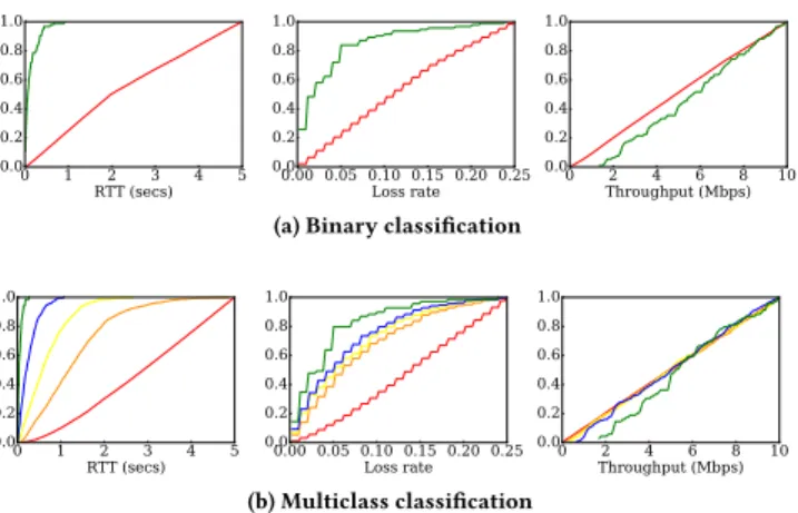
The complete datasets used in our YouTube experiments can be found in [2]. The visual representation in Fig. 1 shows a projection over the two features Round-Trip Time (RTT) and packet loss. For both the binary and the multiclass datasets, the relationship of the QoE labels with network QoS is evident – we can visualize a decision boundary over this projection. Here, points having higher QoE are clustered in the lower regions of the RTT and packet loss space, with an apparent monotonicity in the variation of the QoE labels in particular for the multiclass set. Note here that the projection over the the throughput feature, that we do not included here due to lack of space, did not show such a clear clustering.

Fig. 2 shows the CDF of the pool, P, where the relationship of the QoE w.r.t to the individual network QoS features is highlighted. It can be seen that the effect of RTT and packet loss on the QoE is more pronounced as compared to throughput. In fact, for the case of throughput, the CDF is linear for all classes and shows a threshold effect in case of binary classification, i.e, for all videos

0 1 2 3 4 5 RTT (secs) 0.0 0.2 0.4 0.6 0.8 1.0 0.00 0.05 0.10 0.15 0.20 0.25 Loss rate 0.0 0.2 0.4 0.6 0.8 1.0 0 2 4 6 8 10 Throughput (Mbps) 0.0 0.2 0.4 0.6 0.8 1.0

(a) Binary classification

0 1 2 3 4 5 RTT (secs) 0.0 0.2 0.4 0.6 0.8 1.0 0.00 0.05 0.10 0.15 0.20 0.25 Loss rate 0.0 0.2 0.4 0.6 0.8 1.0 0 2 4 6 8 10 Throughput (Mbps) 0.0 0.2 0.4 0.6 0.8 1.0 (b) Multiclass classification

Figure 2: CDF of the points in the pool

that do not stall (Good points in binary classification), the network has a throughput higher than around 1.6 Mbps which can be un-derstood as the bit rate of the given YouTube 720p video. For such visualizations, if we look at the other two QoS features, we can see that the RTT is always lower than 1 second and packet loss remains below 10% for 90% of the cases. This gives a brief idea on how the network should be provisioned for the given YouTube 720p video to play out without any buffering events.

5

PERFORMANCE ANALYSIS

We compare the performance of the active learning algorithms with uniform sampling where the selection of the instances from the pool P is random. For all scenarios, the same initial training set is used, which comprises of just two points from different classes. Along algorithm execution, each iteration corresponds to picking an instance from the pool and adding it to the training set. After each iteration, the size of the training set increases by one, so the number of iterations also corresponds to the size of the built training set, T. The entire algorithm is run for all the points in the pool and the performance results shown are the average of 20 independent runs. For ease of understanding, the naming convention for the sampling scenarios are mentioned below:

(1) UNIFORM: sampling is random.

(2) LC: sampling is done based on the utility measure of Least Confidence.

(3) MARGIN: sampling is done based on the utility measure of Minimal Margin.

(4) EYNTROPY: sampling is done based on the utility measure of Maximum Entropy

The overall accuracy of the Decision Tree QoE model using the different sampling techniques applied to the binary classification case is shown in Fig. 3a. It can be seen that all the uncertainty sampling techniques have a close performance and they all out-perform uniform sampling by achieving a higher accuracy with a much lower number of samples in the training phase. This ratifies our earlier description of active learning, that training with points closer to the decision boundaries is much more beneficial as com-pared to points away from them. The accuracy starts from its initial

0 2000 4000 6000 8000 10000 Iterations 0.5 0.6 0.7 Accuracy UNIFORM LC MARGIN ENTROPY

(a) Learner accuracy

0 2000 4000 6000 8000 10000 Iterations 0.00 0.25 0.50 0.75 1.00 % of QoE=1.0 Samples UNIFORM LC MARGIN ENTROPY

(b) Cumulative ratio of Good samples

Figure 3: Binary classification results

value of 0.5 (learner predicts initially everything as Bad) and then quickly achieves the optimum accuracy of around 75%, whereas the accuracy using uniform sampling becomes comparable much later on. The performance gain of our methodology can be gauged by the fact that we are now able to build a QoE model much faster and by using almost one order of magnitude fewer experiments com-pared to randomly choosing the network QoS configurations for experimentation (uniform sampling). The reduction in the number of experiments means that we gain in the overall cost involved in building the model.

It has to be noted that this observed value of model prediction accuracy is dependent on the used pool and the validation sets in our experimentation. For different validation sets, the learner accuracy might be slightly different. But still, one can question why the accuracy of the learner is only up to 75%, and does not reach higher values as in prior work on YouTube QoE modeling [5], where the reception ratio was used as a criterion for binary classification of the video as stalling or not stalling. To answer this question, firstly, we argue that the difference between the methodology in this paper and the one in prior work is that the latter uses the network features as observed in the wild, whereas our work considers all possible combinations in a controlled lab environment. Differently speaking, we are validating over challenging scenarios that might not exist in prior work, thus leading to this difference in the result. Indeed, we can see in CDF of our pool (see Fig. 2) that there are points having high bandwidth but still have Bad QoE label because the other parameters of delay and packet loss rate were high to degrade the QoE. For these scenarios, the use of the reception ratio alone is not enough for predicting the QoE. Secondly, our validation sets validate the model built over a smaller experimental space. We deliberately target the ambiguous regions near the borders between classes, where it is expected to have higher classification error.

0 500 1000 1500 2000 2500 Iterations 0.2 0.3 0.4 0.5 Accuracy UNIFORM LC MARGIN ENTROPY

(a) Learner accuracy

0 500 1000 1500 2000 2500 Iterations 1.5 2.0 2.5 Mean Deviation UNIFORM LC MARGIN ENTROPY (b) Mean Deviation

Figure 4: Multiclass classification

From Fig. 1a, we can see that the underlying distribution of the binary labels in the pool is highly unbalanced with all samples from the minority class (i.e., Good class in our case) located in a single

small region in the corner of the experimental space. Due to this reason it can be expected that the active learner tends to focus on this region in picking its points for labeling which would result in picking the instances from the minority class much faster as com-pared to uniform sampling. To verify this, we plot the cumulative ratio of the selected instances from the minority class (Good class in our case) in Fig. 3b, where we can indeed see that the minor points are picked much faster by active sampling as compared to uniform sampling. This results in having adequate number of samples from each class to get a better accuracy.

The results for the multiclass classification case are shown in Fig. 4a for 25% of the pool size to focus on the initial part, where the gain of active sampling over uniform sampling is more visible. A noticeable observation is that the accuracy of the model is much lower than in the binary classification case. The reason being that the number of borders between the multiclass labels is greater as compared to binary classification, so the number of ambiguous regions (the challenged regions where the validation is performed) is also higher, thus the accuracy of the multiclass QoE model is low. Having said that, the converged value of the Mean Deviation shown in Fig. 4b is close to 1, which means that most of the mis-classifications are only to the adjacent classes. As for the active learner’s convergence rate, we can see that it again performs better than uniform sampling as it achieves a lower mean deviation with fewer training samples.

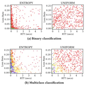
Finally, the difference between the selected instances using active learning (ENTROPY) and uniform sampling is visualized in Fig. 5, at 5% of the pool size. It is evident that in case of uniform sampling, the training set comprises of points scattered throughout the sample space whereas for active learning, points are mostly selected from a region near the decision boundaries. More importantly, unrealistic extreme points of very high RTT/loss rate are seldom sampled by the active learner compared to uniform sampling. Therefore, active learning allows experimentation to be carried out with more realistic network configurations compared to uniform sampling of the space. Hence, we are able to build accurate models quickly, without the need to know any prior information on what a realistic experimental space should be for the given target application.

6

CONCLUSION AND FUTURE WORK

In this paper, we showcased the benefit of using active learning to speed up the process of building QoE models using controlled experimentation. Our work validated active learning over a sample YouTube QoE modeling use case and our results show improvement over conventional uniform sampling of the experimental space. In the future, we plan to incorporate active learning in practice such that the datasets of the QoS-QoE mappings are directly obtained using active learning. Furthermore, future work will also focus on testing the active learning framework with more QoS features (e.g. jitter, re-ordering etc.) and with more applications.

REFERENCES

[1] ACQUA: Application for prediCting Quality of User experience at Internet Access. http://project.inria.fr/acqua/.

[2] Datasets. http://www-sop.inria.fr/diana/acqua/datasets.

[3] Dana Angluin. 1988. Queries and concept learning. Machine Learning 2, 4 (1988). [4] T. Hoßfeld and others. Quantification of YouTube QoE via Crowdsourcing. In

Multimedia (ISM), 2011 IEEE International Symposium on. 494–499.

0 1 2 3 4 5 RTT (secs) 0.00 0.05 0.10 0.15 0.20 0.25 Loss Rate ENTROPY 0 1 2 3 4 5 RTT (secs) 0.00 0.05 0.10 0.15 0.20 0.25 Loss Rate UNIFORM

(a) Binary classification

0 1 2 3 4 5 RTT (secs) 0.00 0.05 0.10 0.15 0.20 0.25 Loss Rate ENTROPY 0 1 2 3 4 5 RTT (secs) 0.00 0.05 0.10 0.15 0.20 0.25 Loss Rate UNIFORM (b) Multiclass classification

Figure 5: Training set points at 5% of the Pool size

[5] Tobias Hoßfeld and others. 2013. Internet Video Delivery in YouTube: From Traffic Measurements to Quality of Experience. Springer Berlin Heidelberg.

[6] ITU. 1998. Subjective audiovisual quality assessment methods for multimedia applications. In ITU-T Recommendation P.911.

[7] Michalis Katsarakis and others. Towards a Causal Analysis of Video QoE from Network and Application QoS. In Proceedings of the Internet QoE 2016. [8] Georgios Exarchakos Menkovski, Vlado and Antonio Liotta. Adaptive testing for

video quality assessment. In Proceedings of Quality of Experience for Multimedia Content Sharing. Lisbon, Portugal, 2011.

[9] Vlado Menkovski and others. Tackling the sheer scale of subjective QoE. In International Conference on Mobile Multimedia Communications. Springer Berlin Heidelberg, 2011.

[10] Ricky K. P. Mok and others. Measuring the quality of experience of HTTP video streaming. In Integrated Network Management 2011. IEEE.

[11] Fabian Pedregosa. 2011. Scikit-learn: Machine learning in Python. Journal of Machine Learning Research (Oct 2011).

[12] Luigi Rizzo. 1997. Dummynet: A Simple Approach to the Evaluation of Network Protocols. SIGCOMM Comput. Commun. Rev. 27, 1 (Jan. 1997), 31–41. [13] B. Settles. Active Learning Literature Survey. Computer Sciences Technical Report

1648, 2010. University of Wisconsin Madison.

[14] T. Spetebroot, S. Afra, N. Aguilera, D. Saucez, and C. Barakat. From network-level measurements to expected quality of experience: The Skype use case. In Measurements Networking (M & N), 2015 IEEE International Workshop on. [15] Byron C. Wallace and others. Active Learning for Biomedical Citation Screening.

In Proceedings of the 16th ACM SIGKDD 2010.

[16] Ting-Fan Wu and others. 2004. Probability Estimates for Multi-class Classification by Pairwise Coupling. J. Mach. Learn. Res. (2004), 31.

[17] P. Ye and D. Doermann. Active Sampling for Subjective Image Quality Assess-ment. In 2014 IEEE Conference on Computer Vision and Pattern Recognition. [18] Xiaoqi Yin and others. A Control-Theoretic Approach for Dynamic Adaptive