HAL Id: cea-02421743
https://hal-cea.archives-ouvertes.fr/cea-02421743
Submitted on 20 Dec 2019
HAL is a multi-disciplinary open access
archive for the deposit and dissemination of
sci-entific research documents, whether they are
pub-lished or not. The documents may come from
teaching and research institutions in France or
abroad, or from public or private research centers.
L’archive ouverte pluridisciplinaire HAL, est
destinée au dépôt et à la diffusion de documents
scientifiques de niveau recherche, publiés ou non,
émanant des établissements d’enseignement et de
recherche français ou étrangers, des laboratoires
publics ou privés.
Monte Carlo Chord Length Sampling for d-dimensional
Markov binary mixtures
C. Larmier, A. Lam, P. Brantley, F. Malvagi, T. Palmer, A. Zoia
To cite this version:
C. Larmier, A. Lam, P. Brantley, F. Malvagi, T. Palmer, et al.. Monte Carlo Chord Length
Sam-pling for d-dimensional Markov binary mixtures. Journal of Quantitative Spectroscopy and Radiative
Transfer, Elsevier, 2018, 204, pp.256-271. �10.1016/j.jqsrt.2017.09.014�. �cea-02421743�
Monte Carlo Chord Length Sampling for d-dimensional Markov binary mixtures
Coline Larmiera, Adam Lamb, Patrick Brantleyc, Fausto Malvagia, Todd Palmerb, Andrea Zoiaa,∗
aDen-Service d’Etudes des R´eacteurs et de Math´ematiques Appliqu´ees (SERMA), CEA, Universit´e Paris-Saclay, 91191 Gif-sur-Yvette, FRANCE. bSchool of Nuclear Science& Engineering, Oregon State University, Corvallis, Oregon, USA.
cLawrence Livermore National Laboratory, P.O. Box 808, Livermore, CA 94551.
Abstract
The Chord Length Sampling (CLS) algorithm is a powerful Monte Carlo method that models the effects of stochastic media on
particle transport by generating on-the-fly the material interfaces seen by the random walkers during their trajectories. This an-nealed disorder approach, which formally consists of solving the approximate Levermore-Pomraning equations for linear particle transport, enables a considerable speed-up with respect to transport in quenched disorder, where ensemble-averaging of the Boltz-mann equation with respect to all possible realizations is needed. However, CLS intrinsically neglects the correlations induced by the spatial disorder, so that the accuracy of the solutions obtained by using this algorithm must be carefully verified with respect to reference solutions based on quenched disorder realizations. When the disorder is described by Markov mixing statistics, such comparisons have been attempted so far only for one-dimensional geometries, of the rod or slab type. In this work we extend these results to Markov media in two-dimensional (extruded) and three-dimensional geometries, by revisiting the classical set of benchmark configurations originally proposed by Adams, Larsen and Pomraning (1) and extended by Brantley (2). In particular,
we examine the discrepancies between CLS and reference solutions for scalar particle flux and transmission/reflection coefficients
as a function of the material properties of the benchmark specifications and of the system dimensionality.
Keywords: Chord Length Sampling, Markov geometries, benchmark, Monte Carlo, Tripoli-4 R, Mercury
1. Introduction
Several applications in nuclear science and engineering in-volve linear particle transport theory in stochastic media.
Ex-amples include neutron diffusion in pebble-bed reactors or
randomly mixed water-vapor phases in boiling water reac-tors (3; 4; 5; 6; 7), and inertial confinement fusion (8; 9; 10). Particle propagation in random media emerges more broadly in material and life sciences and in radiative transport (11; 12; 13; 14; 15; 16; 17). Assuming that particles undergo single-speed transport with isotropic scattering, the angular particle flux ϕ(r, ω) for each physical realization of the system obeys the linear Boltzmann equation
ω · ∇ϕ + Σ(r)ϕ = Σs(r)
Ωd
Z
ϕ(r, ω0
)dω0+ S. (1)
Here r and ω denote the position and direction variables,
re-spectively,Σ(r) being the total cross section and S = S (r, ω)
the source term. The quantityΩd = 2πd/2/Γ(d/2) is the surface
area of the unit sphere in dimension d,Γ(a) being the Gamma
function. The quantitiesΣ(r), Σs(r) and S (r, ω) are in principle
random variables, since the materials composing the traversed medium are assumed to be possibly distributed according to some statistical law. The physical observable of interest is typ-ically the ensemble-averaged angular particle flux hϕ(r, ω)i, or
∗
Corresponding author. Tel.+33 (0)1 69 08 79 76 Email address: [email protected] (Andrea Zoia)
more generally some ensemble-averaged functional hF[ϕ]i of the particle flux, namely,
hϕ(r, ω)i =
Z
P(q)ϕ(q)(r, ω)dq, (2)
where ϕ(q)(r, ω) is the solution of the Boltzmann equation (1)
corresponding to a single realization q, and P(q) is the
station-ary probability of observing the state q for the functionsΣ(q)(r),
Σ(q)
s (r) and S(q)(r, ω) (3; 18).
5
Exact solutions for hF[ϕ]i can be in principle obtained in the following way: first, a realization of the medium is sampled from the underlying mixing statistics; then, the linear transport equation (1) corresponding to this realization is solved by ei-ther deterministic or Monte Carlo methods, and the physical
10
observables of interest F[ϕ] are determined; a sufficiently large
collection of realizations is produced; and ensemble averages are finally taken for the physical observables.
Reference solutions are very demanding in terms of com-putational resources, especially if transport is to be solved by Monte Carlo methods in order to preserve the highest possi-ble accuracy in solving the Boltzmann equation. In principle, it would be thus desirable to directly derive a single equation for the ensemble-averaged flux hϕi. A widely adopted model of random media is the so-called binary stochastic mixing, where only two immiscible materials (say α and β) are present (3). Then, by averaging Eq. (1) over realizations having material α
at r, we obtain the following equation for hϕα(r, ω)i [ω · ∇+ Σα] pαhϕαi= pαΣs,α Ωd Z hϕα(r, ω0)idω0 + pβ,αhϕβ,αi − pα,βhϕα,βi+ pαSα (3)
where pi(r) is the probability of finding the material of index
i at position r. Here pi, j = pi, j(r, ω) represents the
probabil-15
ity per unit length of crossing the interface from material i to material j for a particle located at r and travelling in direction
ω. The quantity hϕi, ji denotes the angular flux averaged over
those realizations where there is a transition from material i to material j for a particle located at r and travelling in direction
20
ω. The cross sections ΣαandΣs,αare those of material α. The
equation for hϕβ(r, ω)i is immediately obtained from Eq. (3) by
permuting the indices α and β. Excluding the special case of particle transport in the absence of scattering, we are thus led to
an infinite hierarchy for hϕαi in Eqs. (3).
25
In order to explicitly derive the ensemble-averaged flux hϕαi,
it is therefore necessary to introduce a closure formula, which will in general depend on the underlying mixing statistics (3; 18; 19). The celebrated Levermore-Pomraning model assumes
for instance hϕα,βi = hϕαi for homogeneous Markov mixing
statistics, with
pi, j(r, ω)= Λpi
i(ω)
, (4)
whereΛi(ω) is the mean chord length for trajectories crossing
material i in direction ω (3). Several generalisations of this model have been later proposed, including higher-order closure schemes (3; 19).
In parallel, a family of Monte Carlo algorithms have been
30
conceived in order to approximate the ensemble-averaged solu-tions to various degrees of accuracy (9; 20; 21). Their com-mon feature is that they allow a simpler treatment of trans-port in stochastic mixtures (typically by neglecting the cor-relations on particle trajectories induced by the spatial
disor-35
der), which might be convenient in practical applications. In this context, a prominent role is played by the so-called Chord Length Sampling (CLS) algorithm, which is supposed to solve the Levermore-Pomraning model for Markovian binary mix-ing (9; 22; 23). The basic idea behind CLS is that the interfaces
40
between the constituents of the stochastic medium are sampled on-the-fly during the particle displacements by drawing the dis-tances to the following material boundaries from a distribution depending on the mixing statistics. The free parameters of the
CLS model are the average chord lengthΛithrough each
mate-45
rial and the volume fraction pi. Since the the spatial
configura-tion seen by each particle is regenerated at each particle flight, the CLS corresponds to an annealed disorder model, as opposed to the quenched disorder of the reference solutions, where the spatial configuration is frozen for all the traversing particles.
50
Generalization of these Monte Carlo algorithms including
par-tial memory effects due to correlations for particles crossing
back and forth the same materials have been also proposed (9). In order to quantify the accuracy of the various approxi-mate models, comparisons with respect to reference solutions
55
are mandatory. For instance, although originally formulated for
Markov statistics, CLS has been extensively applied also to ran-domly dispersed spherical inclusions into background matrices, with application to pebble-bed and very high temperature gas-cooled reactors (20; 21), and several benchmark problems have
60
been examined in two and three dimensions (20; 21; 24; 25). For Markov mixing, a number of benchmark problems com-paring CLS and reference solutions have been proposed in the literature so far (1; 2; 18; 26; 27), with focus exclusively on 1d geometries, either of the rod or slab type. Flat two-dimensional
65
configurations have received less attention (10).
In a series of recent papers, some of the authors have pro-vided reference solutions for particle transport in extruded two-dimensional and full three-two-dimensional random media with Markov statistics (28; 29), where the spatial disorder has
70
been generated by means of homogeneous and isotropic d-dimensional Poisson tessellations (30). In this work, we will compare the CLS simulation results to the reference solu-tions for the classical benchmark problem proposed by Adams, Larsen and Pomraning for transport in stochastic media (1) and
75
revisited by Brantley (2). The case of 1d slab disorder has been considered previously in the literature (1; 2; 18; 26; 27) and will be reported here for the sake of completeness. In addition, we will also consider 2d extruded and full 3d Markov mixing configurations. The physical observables of interest will be the
80
particle flux hϕi, the transmission coefficient hTi and the
re-flection coefficient hRi: we will examine the discrepancies
be-tween reference and CLS simulation results as a function of the benchmark configurations and of the system dimensionality d. In order to verify the consistency of the proposed results, the
85
CLS calculations will be performed by using two independent Monte Carlo implementations of the CLS algorithm, the
for-mer in the Tripoli-4 R code (31), and the latter in the Mercury
code (32; 33).
This paper is organized as follows: in Sec. 2 we will recall
90
the benchmark specifications that will be used in this work. In Secs. 3 and 4 we will detail the methods and the algorithms that we have adopted in order to produce reference and CLS results, respectively. Simulation findings will be illustrated and discussed in Sec. 5. Conclusions will be finally drawn in Sec. 6.
95
2. Benchmark specifications
In order for the paper to be self-contained, we start by re-calling the benchmark specifications that have been selected for this work, which are essentially taken from those originally pro-posed in (1) and (18), and later extended in (2; 26; 27).
100
We consider single-speed linear particle transport through a stochastic binary medium with homogeneous Markov mixing. The medium is non-multiplying, with isotropic scattering. The
geometry consists of a cubic box of side L = 10 (in arbitrary
units), with reflective boundary conditions on all sides of the box except two opposite faces (say those perpendicular to the x
axis), where leakage boundary conditions are imposed1. Two
1In (1) and (18), system sizes L= 0.1 and L = 1 were also considered, but in this work we will focus on the case L= 10, which leads to more physically relevant configurations.
kinds of non-stochastic sources will be considered: either an imposed normalized incident angular flux on the leakage
sur-face at x = 0 (with zero interior sources), or a distributed
ho-mogeneous and isotropic normalized interior source (with zero incident angular flux on the leakage surfaces). Following the notation in (2), the benchmark configurations pertaining to the former kind of source will be called suite I, whereas those per-taining to the latter will be called suite II. The material prop-erties for the Markov mixing are entirely defined by assigning
the average chord length for each material i = α, β, namely
Λi, which in turn allows deriving the homogeneous probability
piof finding material i at an arbitrary location within the box,
namely
pi= Λ
i
Λi+ Λj
. (5)
By definition, the material probability piyields the volume
frac-tion for material i. The cross secfrac-tions for each material will
be denoted as customaryΣifor the total cross section andΣs,i
for the scattering cross section. The average number of par-ticles surviving a collision in material i will be denoted by
105
ci = Σs,i/Σi ≤ 1. The physical parameters for the benchmark
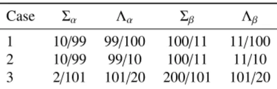
configurations are recalled in Tabs. 1 and 2: the benchmark specifications include three cases (numbered 1, 2 and 3,
cor-responding to different materials), and three sub-cases (noted
a, b and c, corresponding to different ci for a given material)
110
for each case (1). The so-called atomic mix limit (3), where one assumes that the statistical disorder can be approximated by simply taking a full homogenization of the physical prop-erties based on the ensemble-averaged cross sections, has been
examined, e.g., in (2) for d= 1 and in (28) for d = 2 and d = 3
115
and will not be considered here.
Case Σα Λα Σβ Λβ
1 10/99 99/100 100/11 11/100
2 10/99 99/10 100/11 11/10
3 2/101 101/20 200/101 101/20
Table 1: Material parameters for the three cases of the benchmark configura-tions.
Sub-case a b c
cα 0 1 0.9
cβ 1 0 0.9
Table 2: Scattering probabilities for the three sub-cases of the benchmark con-figurations.
The physical observables of interest for the proposed bench-mark will be the ensemble-averaged outgoing particle cur-rents hJi on the two surfaces with leakage boundary
con-ditions, the ensemble-averaged scalar particle flux hϕ(x)i =
120
hR R R ϕ(r, ω)dωdydzi along 0 ≤ x ≤ L, and the total scalar
flux hϕi = hR ϕ(x)dxi. For the suite I configurations, the
out-going particle current on the side opposite to the imposed cur-rent source will represent the ensemble-averaged transmission
coefficient, namely, hTi = hJx=Li, whereas the outgoing
parti-125
cle current on the side of the current source will represent the
ensemble-averaged reflection coefficient, namely, hRi = hJx=0i.
For the suite II configurations, the outgoing currents on oppo-site faces are expected to be equal (within statistical fluctua-tions), for symmetry reasons. In this case, we also introduce
130
the average leakage current hLi= h(T + R)/2i.
3. Reference solutions
For particle transport in the presence of quenched disorder with Markov mixing, the reference solutions for the ensemble-averaged scalar particle flux hϕ(x)i and the currents hRi and hT i
135
have been thoroughly described in (28). Here we will briefly recall the methods that have been used.
3.1. Poisson tessellations
Random tessellations are stochastic aggregates of disjoint and space-filling cells obeying a given distribution (34).
Pois-140
son tessellations are obtained by partitioning a domain of a d-dimensional space by sampling (d − 1)-dimensional hyper-planes from an auxiliary Poisson process (34; 35; 36). An ex-plicit construction amenable to Monte Carlo realizations for two-dimensional homogeneous and isotropic Poisson
geome-145
tries of finite size has been established in (37). A generalization of this algorithm to d-dimensional domains has been recently proposed (38). The construction of Poisson stochastic geome-tries depends on a single free parameter ρ, which takes the name of tessellation density, and is such that an arbitrary segment of
150
length s will have on average ρs intersections with the random hyper-planes.
The algorithm for the 1d slab tessellations is recalled in (1), based on the Poisson process on the line. For the 2d extruded tessellations, we begin by creating an isotropic Poisson
tessel-155
lation of a square of side L, according to the algorithm detailed in (39). The full geometrical description for the cube is simply achieved by extruding the random polygons of the plane along the orthogonal (say z) axis. The algorithm for 3d tessellations of a cube of side L by drawing random planes has been detailed
160
in (30).
Isotropic Poisson geometries satisfy a Markov property: for domains of infinite size, arbitrary drawn lines will be cut by the (d −1)-surfaces of the d-polyhedra into segments whose lengths ` are exponentially distributed, with average chord length h`i =
165
1/ρ (34). The quantityΛ = 1/ρ intuitively defines the
correla-tion length of the Poisson geometry, i.e, the typical linear size of a volume composing the random tessellation.
3.2. Colored stochastic geometries
Binary Markov mixtures required for the benchmark specifi-cations are obtained as follows: first, a d-dimensional Poisson tessellation is constructed as described above. Then, each poly-hedron of the geometry is assigned a material composition by
formally attributing a distinct ‘color’, say α or β, with
asso-ciated complementary probabilities pα and pβ = 1 − pα (3).
This gives rise to (generally) non-convex α and β clusters, each composed of a random number of convex polyhedra. It can
be shown that the average chord length Λα through clusters
with composition α is related to the correlation lengthΛ of the
geometry viaΛ = (1 − pα)Λα, and for Λβ we similarly have
Λ = pαΛβ. This yields 1/Λα+ 1/Λβ = 1/Λ, and we recover
pα =ΛΛ
β =
Λα
Λα+ Λβ. (6)
Based on the formulas above, and using ρ = 1/Λ, the
param-170
eters of the colored Poisson geometries corresponding to the benchmark specifications provided in Tab. 1 are easily derived. 3.3. Particle transport and ensemble averages
For each benchmark case and sub-case, a large number M of geometries has been generated, and the material properties have been attributed to each volume as described above. Then, for each realization k of the ensemble, linear particle transport has been simulated by using the production Monte Carlo code
Tripoli-4 R
, developed at CEA (31). Tripoli-4 R is a
general-purpose stochastic transport code capable of simulating the propagation of neutral and charged particles with continuous-energy cross sections in arbitrary geometries. In order to com-ply with the benchmark specifications, constant cross sections adapted to mono-energetic transport and isotropic angular dis-tributions have been prepared. The number of simulated
parti-cle histories per configuration is 106. For a given physical
ob-servable O, the benchmark solution is obtained as the ensemble average hOi= 1 M M X k=1 Ok, (7)
where Okis the Monte Carlo estimate for the observable O
ob-tained for the k-th realization. Specifically, currents Rkand Tkat
175
a given surface are estimated by summing the statistical weights
of the particles crossing that surface. Scalar fluxes ϕk(x) have
been tallied using the standard track length estimator over a
pre-defined spatial grid containing 102 uniformly spaced meshes
along the x axis.
180
The error affecting the average observable hOi results from two separate contributions, the dispersion
σ2 G= 1 M M X k=1 Ok2− hOi2 (8)
of the observables exclusively due to the stochastic nature of the geometries and of the material compositions, and
σ2 O= 1 M M X k=1 σ2 Ok, (9)
which is an estimate of the variance due to the stochastic nature
of the Monte Carlo method for particle transport, σ2
Ok being the
dispersion of a single calculation (21; 20). The statistical error on hOi is then estimated as
σ[hOi] = s σ2 G M + σ 2 O. (10)
The number M of realizations that have been used for the Monte Carlo simulations has been chosen as follows: for 1d
slab tessellations, we have taken M = 104(except for the case
2a for the suite II, where the number of geometries has been
increased to M = 5 × 10⁴ in order to reduce the statistical
185
fluctuations); for the 2d extruded tessellations, we have taken
M = 4 × 10³; finally, for the 3d tessellations we have taken
M = 103. Actually, increasing the dimension d implies a
bet-ter statistical mixing (in other words, a single realization is more representative of the average behaviour), at the expense
190
of increasing the computational burden (each realization takes longer both for generation and for Monte Carlo transport).
Transport calculations have been run on a cluster based at CEA, with Intel Xeon E5-2680 V2 2.8 GHz processors. The average computer time globally increases as a function of
di-195
mension, but depends also on the correlation lengths, volume fractions, and material properties such as cross sections and scattering probabilities. For the simulations discussed here we have largely benefited from a feature implemented in the code
Tripoli-4 R, namely the possibility of reading pre-computed
200
connectivity maps for the volumes composing the geometry. During the generation of the Poisson tessellations, care has been taken so as to store the indices of the neighbouring volumes for each realization, which means that during the geometrical tracking a particle will have to find the following crossed
vol-205
ume in a list that might be considerably smaller than the total number of random volumes composing the box (depending on the features of the random geometry).
4. The Chord Length Sampling approach
Reference solutions based on the quenched disorder
ap-210
proach are computationally expensive, so that intensive
re-search efforts have been devoted to the development of Monte
Carlo-based annealed disorder models capable of approximat-ing the ensemble observables on-the-fly, i.e., with a sapproximat-ingle par-ticle transport simulation. The pioneering work by Zimmerman
215
and Adams (8; 9) has led to a family of algorithms that go now under the name of Chord Length Sampling methods. In particu-lar, it has been shown that the standard form of the CLS (Algo-rithm A in (9)) formally solves the Levermore-Pomraning equa-tions, i.e., Eq. (3) with the closure formula (4), corresponding
220
to Markov mixing with the approximation that memory of the crossed material interfaces is lost at each particle flight (22; 23). Algorithm A proceeds as follows (9): each particle history begins by sampling position, angle and velocity from the spec-ified source, as customary. Moreover, the particle is assigned
225
a supplementary attribute, the material label, which is sampled
from the probability pi. Then we need to compute three
dis-tances, denoted respectively `b, `c, and `i. The quantity `b is
direction of the particle. The quantity `cis the distance to the
230
next collision, which is determined by using the material cross section that has been chosen at the previous step: if the particle
has a material α, e.g., then `cwill be drawn from an
exponen-tial distribution of parameter 1/Σα. Finally, the quantity `iis the
distance to the next material interface, which is sampled from
235
an exponential distribution with parameterΛα, i.e., the average
chord length of material α, if the particle has a material label α (whence the name of CLS).
Then, the minimum distance among `b, `c and `i must be
selected: if the minimum is `b, the particle is moved along a
240
straight line until it hits the external boundary; if the minimum
is `c, the particle is moved to the collision point, and the
out-going particle features are selected according to the collision kernel pertaining to the current material label. If the minimum
is `i, the particle is moved to the interface between the two
ma-245
terials, and the material label is switched. If the particle is not
absorbed, a new set of distances `b, `cand `i are determined.
During the time spent within the random medium, the particle will be thus either colliding within a random chunk, or crossing the interface between two chunks; the particle will ultimately
250
get absorbed in one of the chunks, or escape out of the bound-aries of the random medium. The Monte Carlo estimators for the scalar flux and the currents are the same as those for the reference solutions described above.
As observed above, Algorithm A assumes that the particle
255
has no memory of its past history, and in particular the crossed interfaces are immediately forgotten (which is coherent with the closure formula of the Levermore-Pomraning model). In this respect, CLS is an approximation of the exact treatment of disorder-induced spatial correlations (actually, it can be shown
260
that CLS is exact only for pure absorbers). As a result, Algo-rithm A is expected to be less accurate in the presence of strong scatterers with optically thick mean material chunk length. 4.1. Slab geometries
For mono-energetic particle transport in slab geometries with isotropic scattering, the Boltzmann equation (1) yields
µ∂ ∂xϕ + Σ(x)ϕ = Σs(x) 2 Z 1 −1 dµ0ϕ(x, µ0), (11)
where ϕ = ϕ(x, µ) is the angular particle flux for particles at
265
position x with a direction cosine µ= cos(θ) with respect to the
xaxis. The source and the boundary conditions depend on the
benchmark specifications.
Correspondingly, the CLS algorithm that formally solves the Levermore-Pomraning model as applied to Eq. 11 is the
fol-lowing. For suite I, the source particle position is set to x= 0,
and the direction cosine is sampled from a cosine distribution, namely,
µ = pξ, (12)
where ξ is a uniform random number in [0, 1), in order to en-sure the isotropic incident flux condition. For suite II, the start-ing position x is sampled uniformly in [0, L], and the direc-tion cosine is sampled uniformly in [−1, 1] in order to ensure the uniform and isotropic source condition. According to the
Levermore-Pomraning prescription, the distance to material in-terfaces for a particle in material α is sampled from an expo-nential distribution as follows:
di= −
Λα
|µ| ln(1 − ξ), (13)
where the factor 1/|µ| accounts for the projection of the distance along the x axis. The distance to the next collision is
sam-270
pled from the exponential distribution of parameter 1/Σα(x),
and the distance to the boundary is computed as customary. For isotropic scattering, the cosine direction after collision is sam-pled uniformly in [−1, 1].
4.2. Two-dimensional extruded geometries
275
Assuming again mono-energetic particle transport with
isotropic scattering, the Boltzmann equation for
two-dimensional geometries extruded in the z axis direction yields q 1 − µ2cos(φ)∂ ∂xϕ + q 1 − µ2sin(φ)∂ ∂yϕ = Σ(x, y)ϕ +Σs(x, y) 4π Z 1 −1 dµ0Z 2π 0 dφ0ϕ(x, y, µ0, φ0 ), (14)
where ϕ = ϕ(x, y, µ, φ) is the angular particle flux for particles
being at position x, y with a direction cosine µ = cos(θ) with
respect to the z axis and a polar angle φ with respect to the x axis.
The CLS algorithm that formally corresponds to solving the Levermore-Pomraning model as applied to Eq. 14 is the
follow-ing. For suite I, the source particle positions are set to x= 0 and
ytaken uniformly in [0, L]. Then we sample a direction cosine
µ0(with respect to the x axis) from
µ0= pξ (15)
where ξ is taken in [0, 1), and a polar angle φ0(with respect to
the y axis) uniform in [0, 2π]. The initial particle direction is
ω0= µ0 Q, p 1 − µ02cos(φ0) Q , (16) with Q= q µ02+ (1 − µ02) cos2(φ0), (17)
in order to ensure the isotropic incident flux condition, and the
initial direction cosine µ0is defined by
µ0=
q
1 − µ02sin(φ0). (18)
For suite II, the starting positions x, y are sampled uniformly in [0, L] × [0, L], the direction cosine µ is sampled uniformly in [−1, 1] and the polar angle φ is sampled uniformly in [0, 2π] in order to ensure the uniform and isotropic source condition, which yields the initial particle direction
According to the Levermore-Pomraning prescription, the dis-tance to material interfaces for a particle in material α is sam-pled from an exponential distribution as follows:
di= − Λ
α
p
1 − µ2 ln(1 − ξ), (20)
where the factor 1/p1 − µ2 again accounts for the projection
of the distance on the x − y plane. The distance to the next col-lision is sampled from the exponential distribution of
parame-ter 1/Σα(x, y), and the distance to the boundary is computed as
customary. For isotropic scattering, the cosine direction µ after collision is sampled uniformly in [−1, 1], and the polar angle φ is sampled uniformly in [0, 2π]; the particle direction is then given by
ω = {cos(φ), sin(φ)} . (21)
4.3. Three-dimensional geometries
280
The Boltzmann equation for mono-energetic transport with isotropic scattering in three-dimensional geometries yields
q 1 − µ2cos(φ) ∂ ∂x + q 1 − µ2sin(φ)∂ ∂y +µ ∂ ∂z ! ϕ = Σ(x, y, z)ϕ + Σs(x, y, z) 4π Z 1 −1 dµ0 Z 2π 0 dφ0ϕ(x, y, z, µ0, φ0 ), (22)
where ϕ= ϕ(x, y, z, µ, φ) is the angular particle flux for particles
being at position x, y, z with a direction cosine µ= cos(θ) with
respect to the z axis and a polar angle φ with respect to the x axis.
The CLS algorithm that formally corresponds to solving the Levermore-Pomraning model as applied to Eq. 22 is the
fol-lowing. For suite I, the source particle positions are set to x= 0
and y, z taken uniformly in [0, L] × [0, L]. Then we sample a
direction cosine µ0(with respect to the x axis) from
µ0= pξ (23)
where ξ is taken in [0, 1), and a polar angle φ0(with repect to
the y axis) uniform in [0, 2π]. The initial particle direction is
ω0=
(
µ0,q1 − µ02cos(φ0),q1 − µ02sin(φ0)
)
(24) in order to ensure the isotropic incident flux condition. For
suite II, the starting positions x, y, z are sampled uniformly in
[0, L] × [0, L] × [0, L], the direction cosine µ is sampled uni-formly in [−1, 1] and the polar angle is sampled uniuni-formly in [0, 2π] in order to ensure the uniform and isotropic source con-dition, which yields the initial particle direction
ω0= ( q 1 − µ2cos(φ), q 1 − µ2sin(φ), µ ) . (25)
According to the Levermore-Pomraning prescription, the dis-tance to material interfaces for a particle in material α is sam-pled from an exponential distribution as follows:
di= −Λαln(1 − ξ). (26)
The distance to the next collision is sampled from the
exponen-tial distribution of parameter 1/Σα(x, y, z), and the distance to
the boundary is computed as customary. For isotropic scatter-ing, the cosine direction µ after collision is sampled uniformly in [−1, 1], and the polar angle φ is sampled uniformly in [0, 2π]; the particle direction is then given by
ω =( q1 − µ2cos(φ), q 1 − µ2sin(φ), µ ) . (27) 5. Simulation results 285
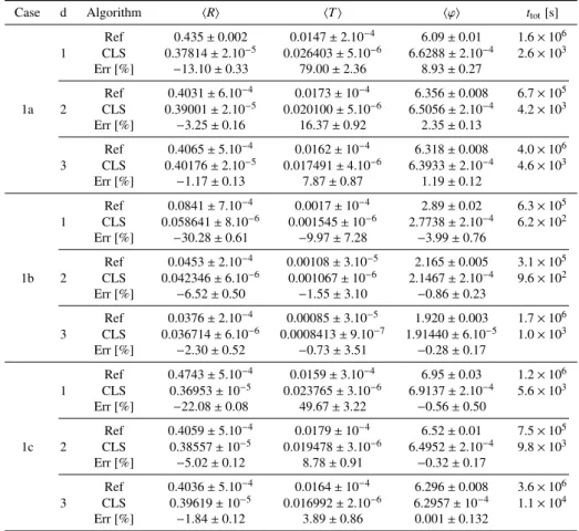
The simulation results for the total scalar flux hϕi, the
trans-mission coefficient hTi and the reflection coefficient hRi are
provided in Tabs. 3 to 5 for the benchmark cases corresponding to suite I, and in Tabs. 6 to 8 for the benchmark cases corre-sponding to suite II, respectively. The reference solutions are
290
taken from reference (28).
The CLS results have been obtained with both Tripoli-4 R
and Mercury Monte Carlo codes by following the procedure
de-scribed above. We will denote by σCLS[O] the resulting
statis-tical uncertainty associated to each physical observable O. For
295
the Tripoli-4 R CLS simulations of the d-dimensional
bench-mark configurations we have used 109 particles (103 replicas
with 106particles per replica). Mercury is a Monte Carlo
par-ticle transport code being developed at Lawrence Livermore National Laboratory (32; 33). The Monte Carlo
Levermore-300
Pomraning CLS algorithm was previously implemented in Mer-cury (25) in a manner consistent with the algorithmic descrip-tions in (9; 2) and Sec. 4. The Mercury Levermore-Pomraning implementation has been demonstrated (25) to accurately re-produce the independent one-dimensional slab geometry Monte
305
Carlo Levermore-Pomraning results in (2). We modelled the three-dimensional benchmark suites I and II using the Mercury
Levermore-Pomraning CLS implementation with 109 particle
histories. We obtained results that are generally statistically
equivalent to the Tripoli-4 R CLS results to typically within
310
three standard deviations for the reflection and transmission
co-efficients and the scalar flux distributions (agreement to
typi-cally four to five digits). For this paper, we will present only
the Tripoli-4 R simulation results. Computer times for the
ref-erence and CLS solutions are also provided in the same tables:
315
not surprisingly, the CLS approach is much faster than the ref-erence method, since a single transport simulation is needed.
As a general remark, the accuracy of CLS with respect to ref-erence solutions increases with increasing system dimensional-ity d. This is expected on physical grounds, since the higher d
320
and the smaller is the impact of the spatial correlations: a par-ticle undergoing back-scattering is less likely to cross exactly the same material interface as the one crossed during the pre-vious flight. In other words, the approximations introduced in the CLS algorithm by neglecting spatial correlations will have
325
a weaker effect on particle transport. Nonetheless, simulation
results show a few exceptions among the examined configura-tions. Moreover, the accuracy of CLS also generally improves when increasing the tessellation density, i.e., decreasing the av-erage chord length: configurations pertaining to case 1 globally
show a better agreement than those of case 2, and those of case 2 show a better agreement than those of case 3.
The effects of system dimensionality on the discrepancies
be-tween CLS and exact solutions are stronger for configurations with smaller average chord lengths. This behaviour is again
335
consistent with the fact that increasing the chord length induces larger chunks of materials, and for chunks that span a large frac-tion of the entire geometry the impact of dimensionality must be rather weak: in this regime, particle transport is mostly influ-enced by the material volume fractions (i.e., the coloring
prob-340
ability).
The behaviour of suite II configurations is quite similar to that of suite I configurations, and no specific trend due to the
source and/or initial conditions can be easily detected.
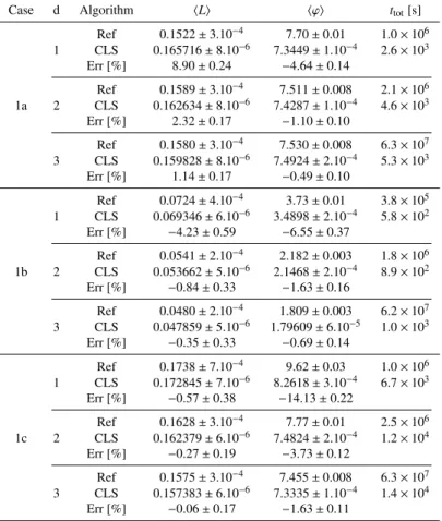
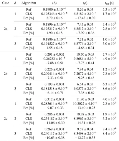
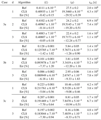
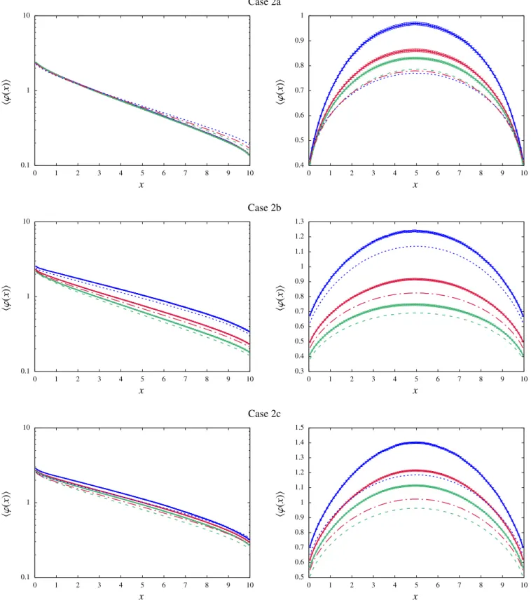
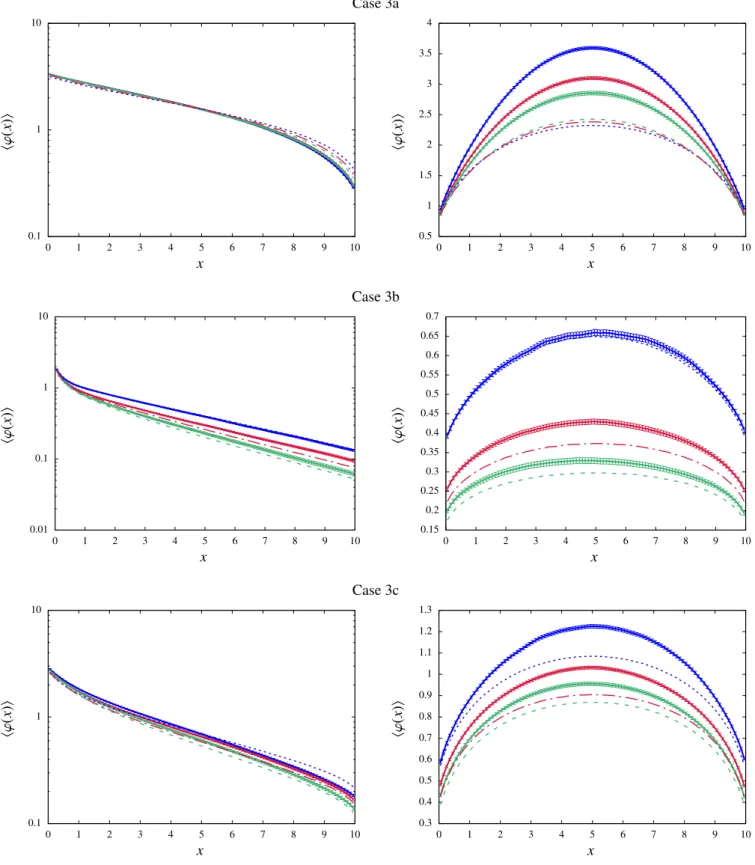
The spatial scalar flux hϕi within the box is illustrated in Figs. 1 to 3 for case 1 to case 3, respectively. The discrep-ancies between CLS and reference solutions for this observable have the same behaviour as for the scalar quantities described above. The discrepancy decreases with increasing system di-mensionality and with decreasing average chord length. For
dense geometries (case 1) the effects of dimensionality on the
discrepancy are rather strong, and become less appreciable for
less dense geometries. The kind of source and/or initial
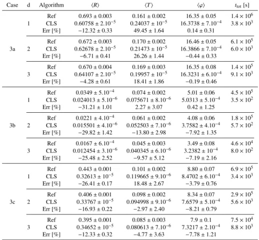
condi-tions plays again a minor role. This analysis is confirmed by plotting the differences ∆[hϕ(x)i] between reference and CLS solutions (see Figs. 4 to 6 for case 1 to case 3, respectively).
Since both reference and CLS solutions are affected by a
sta-tistical uncertainty, the error bars on∆[hϕ(x)i] have been
com-puted by taking the combined variance
σ[∆[O]] = qσ2[hOi]+ σ2
CLS[O] (28)
for each observable O.
345
6. Conclusions
The Chord Length Sampling algorithm efficiently provides
approximate ensemble-averaged observables corresponding to the Levermore-Pomraning model for Markovian binary mixing. The interfaces between the constituents of the random medium
350
are sampled on-the-fly during the particle displacements by drawing the distances to the following material boundaries from a distribution depending on the mixing statistics: the corre-lations on particle trajectories induced by the spatial disorder are thus neglected. Comparisons of CLS solutions with respect
355
to reference results are mandatory in order to quantify the de-gree of approximations introduced in these models. For Markov mixing, a number of benchmark problems have been proposed in the literature for this purpose, but so far analyses have been conducted in one-dimensional media of the rod or slab type.
360
Based on the set of reference solutions for particle transport in two and three dimensional random media with Markov statis-tics that we have derived in a series of recent papers, in this work we have compared CLS simulation results to the refer-ence solutions for the classical benchmark problem proposed
365
by Adams, Larsen and Pomraning, and recently revisited by
Brantley, for particle propagation in stochastic media with bi-nary Markov mixing. In particular, we have examined the evo-lution of the particle flux, the transmission coefficient and the
reflection coefficient as a function of the benchmark
configura-370
tions and of the system dimension d.
Two main trends have been detected: the accuracy of CLS al-gorithm with respect to reference solutions generally increases with increasing system dimensionality. Moreover, the accuracy of the CLS algorithm increases for decreasing average chord
375
length, i.e., for denser stochastic tessellations. The impact of dimensionality is particularly relevant for case 1 configurations (which have smaller chord lengths), and progressively dimin-ishes for configurations having larger material chunks. The considerations presented in this paper, although derived strictly
380
speaking for the Adams, Larsen and Pomraning benchmark considered here, seem to be quite general.
This work represents a first step towards extensive compar-isons between CLS and reference solutions for Markov
mix-ing statistics in higher dimensions. Furthermore, extension
385
of these comparisons to reference solutions for other types of d-dimensional mixing statistics based on spatial tessellations (such as the Poisson-Voronoi model presented in (29)) would be interesting topics for future research.
Acknowledgements
390
TRIPOLI-4 R is a registered trademark of CEA. C. Larmier,
A. Zoia and F. Malvagi wish to thank ´Electricit´e de France
(EDF) for partial financial support. Work of P. Brantley per-formed under the auspices of the U. S. Department of Energy by Lawrence Livermore National Laboratory under Contract
DE-395
AC52-07NA27344.
References
[1] Adams ML, Larsen EW, Pomraning GC. Benchmark results for particle transport in a binary Markov statistical medium. J Quant Spectrosc Radiat Transfer 1989;42:253-66.
400
[2] Brantley PS. A benchmark comparison of Monte Carlo particle trans-port algorithms for binary stochastic mixtures. J Quant Spectrosc Radiat Transfer 2011;112:599-618.
[3] Pomraning GC. Linear kinetic theory and particle transport in stochastic mixtures. River Edge, NJ, USA: World Scientific Publishing; 1991.
405
[4] Larsen EW, Vasques R. A generalized linear Boltzmann equation for non-classical particle transport. J Quant Spectrosc Radiat Transfer 2011:112;619-31.
[5] Levermore CD, Pomraning GC, Sanzo DL, Wong J. Linear transport the-ory in a random medium. J Math Phys 1986;27:2526-36.
410
[6] Sanchez R. Linear kinetic theory in stochastic media. J Math Phys 1988;30:2498-2511.
[7] Levermore CD, Pomraning GC, Wong J. Renewal theory for transport processes in binary statistical mixtures. J Math Phys 1988;29:995-1004. [8] Zimmerman GB. Recent developments in Monte Carlo techniques.
415
Lawrence Livermore National Laboratory Report UCRL-JC-105616; 1990.
[9] Zimmerman GB, Adams ML. Algorithms for Monte Carlo particle trans-port in binary statistical mixtures. Trans Am Nucl Soc 1991:66;287. [10] Haran O, Shvarts D, Thieberger R. Transport in 2D scattering stochastic
420
media: simulations and models. Phys Rev E 2000:61;6183-89.
[11] Torquato S. Random heterogeneous materials: microstructure and macro-scopic properties. New York, USA: Springer-Verlag; 2002.
[12] Barthelemy P, Bertolotti J, Wiersma DS. A L´evy flight for life. Nature 2009:453,495-98.
425
[13] Davis AB, Marshak A. Photon propagation in heterogeneous opti-cal media with spatial correlations. J Quant Spectrosc Radiat Transfer 2004:84;3-34.
[14] Kostinski AB, Shaw RA. Scale-dependent droplet clustering in turbulent clouds. J Fluid Mech 2001:434;389-98.
430
[15] Malvagi F, Byrne RN, Pomraning GC, Somerville RCJ. Stochastic radia-tive transfer in partially cloudy atmosphere. J Atm Sci 1992:50;2146-58. [16] Tuchin V. Tissue optics: light scattering methods and instruments for
medical diagnosis. Cardiff, UK: SPIE Press; 2007.
[17] Brantley PS, Gentile NA, Zimmerman GB. Beyond
Levermore-435
Pomraning for implicit Monte Carlo radiative transfer in binary stochas-tic media. In: Proceedings of M&C 2017 - International Conference on Mathematics & Computational Methods Applied to Nuclear Science & Engineering, Jeju, Korea. April 16-20, 2017 [on USB].
[18] Zuchuat O, Sanchez R, Zmijarevic I, Malvagi F. Transport in renewal
440
statistical media: benchmarking and comparison with models. J Quant Spectrosc Radiat Transfer 1994;51:689-722.
[19] Su B, Pomraning GC. Modification to a previous higher order model for particle transport in binary stochastic media. J Quant Spectrosc Radiat Transfer 1995;54:779-801.
445
[20] Donovan TJ, Sutton TM, Danon Y. Implementation of Chord Length Sampling for transport through a binary stochastic mixture. In: Proceed-ings of the nuclear mathematical and computational sciences: a century in review, a century anew, Gatlinburg, TN. La Grange Park, IL: American Nuclear Society; April 6-11, 2003 [on CD-ROM].
450
[21] Donovan TJ, Danon Y. Application of Monte Carlo chord-length sam-pling algorithms to transport through a two-dimensional binary stochastic mixture. Nucl Sci Eng 2003;143:226-39.
[22] Sahni DC. Equivalence of generic equation method and the phenomeno-logical model for linear transport problems in a two-state random
scatter-455
ing medium. J Math Phys 1989:30; 1554-9.
[23] Sahni DC. An application of reactor noise techniques to neutron transport problems in a random medium. Ann Nucl Energy 1989:16;397-408. [24] Brantley PS, Martos JN. Impact of spherical inclusion mean chord length
and radius distribution on three-dimensional binary stochastic medium
460
particle transport. In: Proceedings of the international conference on mathematics, computational methods & reactor physics (M&C2011), Rio de Janeiro, RJ, Brazil; May 8-12, 2011 [on CD-ROM].
[25] Brantley PS. Benchmark investigation of a 3D Monte Carlo Levermore-Pomraning algorithm for binary stochastic media. Trans Am Nucl Soc
465
2014;111:655-58. Anaheim, CA; November 9-13 2014. [on CD-ROM]. [26] Brantley PS, Palmer TS. Levermore-Pomraning model results for an
in-terior source binary stochastic medium benchmark problem. In: Pro-ceedings of the international conference on mathematics, computational methods & reactor physics (M&C2009), Saratoga Springs, New York.
470
La Grange Park, IL: American Nuclear Society; May 3-7, 2009 [on CD-ROM].
[27] Brantley PS. A comparison of Monte Carlo particle transport algo-rithms for binary stochastic mixtures. In: Proceedings of the international conference on mathematics, computational methods & reactor physics
475
(M&C2009), Saratoga Springs, New York. La Grange Park, IL: Amer-ican Nuclear Society; May 3-7, 2009 [on CD-ROM].
[28] Larmier C, Hugot FX, Malvagi F, Mazzolo A, Zoia A. Benchmark so-lutions for transport in d-dimensional Markov binary mixtures. J Quant Spectrosc Radiat Transfer 2017:189;133148.
480
[29] Larmier C, Zoia A, Malvagi F, Dumonteil E, Mazzolo A. Monte Carlo particle transport in random media: The effects of mixing statistics. J Quant Spectrosc Radiat Transfer 2017:196;27086.
[30] Larmier C, Dumonteil E, Malvagi F, Mazzolo A, Zoia A. Finite-size effects and percolation properties of Poisson geometries. Phys Rev E
485
2016:94;012130.
[31] Brun E, Damian F, Diop CM, Dumonteil E, Hugot FX, Jouanne C, Lee YK, Malvagi F, Mazzolo A, Petit O, Trama JC, Visonneau T, Zoia A. TRIPOLI-4, CEA, EDF and AREVA reference Monte Carlo code. Ann Nucl Energy 2015:82;151-60.
490
[32] Brantley PS, Bleile RC, Dawson SA, McKinley MS, O’Brien MJ, Pozulp MM, Procassini RJ, Richards DF, Sepke SM, Stevens DE, Walsh JA. Mer-cury User Guide: Version 5.6. Lawrence Livermore National Laboratory Report LLNL-SM-560687 (Modification #12) 2017.
[33] Brantley PS, Bleile RC, Dawson SA, Gentile NA, McKinley MS, O’Brien
495
MJ, Pozulp MM, Richards DF, Stevens DE, Walsh JA, Childs H. LLNL Monte Carlo Transport Research Efforts for Advanced Computing Archi-tectures. In: Proceedings of M&C 2017 - International Conference on Mathematics & Computational Methods Applied to Nuclear Science & Engineering, Jeju, Korea. April 16-20, 2017 [on USB].
500
[34] Santal´o LA. Integral geometry and geometric probability. Reading, MA, USA: Addison-Wesley; 1976.
[35] Miles RE. Random polygons determined by random lines in a plane. Proc Nat Acad Sci USA 1964: 52; 901-7.
[36] Miles RE. The random division of space. Suppl Adv Appl Prob
505
1972:4;243-66.
[37] Switzer P. Random set process in the plane with Markov property. Ann Math Statist 1965:36;1859-63.
[38] Ambos AYu, Mikhailov GA. Statistical simulation of an exponentially correlated many-dimensional random field. Russ J Numer Anal Math
510
Modelling 2011:26;263-73.
[39] Lepage T, Delaby L, Malvagi F, Mazzolo A. Monte Carlo simulation of fully Markovian stochastic geometries. Prog Nucl Sci Techn 2011:2;743-48.
Case d Algorithm hRi hT i hϕi ttot[s] Ref 0.435 ± 0.002 0.0147 ± 2.10−4 6.09 ± 0.01 1.6 × 10⁶ 1 CLS 0.37814 ± 2.10−5 0.026403 ± 5.10−6 6.6288 ± 2.10−4 2.6 × 10³ Err [%] −13.10 ± 0.33 79.00 ± 2.36 8.93 ± 0.27 Ref 0.4031 ± 6.10−4 0.0173 ± 10−4 6.356 ± 0.008 6.7 × 10⁵ 1a 2 CLS 0.39001 ± 2.10−5 0.020100 ± 5.10−6 6.5056 ± 2.10−4 4.2 × 10³ Err [%] −3.25 ± 0.16 16.37 ± 0.92 2.35 ± 0.13 Ref 0.4065 ± 5.10−4 0.0162 ± 10−4 6.318 ± 0.008 4.0 × 10⁶ 3 CLS 0.40176 ± 2.10−5 0.017491 ± 4.10−6 6.3933 ± 2.10−4 4.6 × 10³ Err [%] −1.17 ± 0.13 7.87 ± 0.87 1.19 ± 0.12 Ref 0.0841 ± 7.10−4 0.0017 ± 10−4 2.89 ± 0.02 6.3 × 10⁵ 1 CLS 0.058641 ± 8.10−6 0.001545 ± 10−6 2.7738 ± 2.10−4 6.2 × 10² Err [%] −30.28 ± 0.61 −9.97 ± 7.28 −3.99 ± 0.76 Ref 0.0453 ± 2.10−4 0.00108 ± 3.10−5 2.165 ± 0.005 3.1 × 10⁵ 1b 2 CLS 0.042346 ± 6.10−6 0.001067 ± 10−6 2.1467 ± 2.10−4 9.6 × 10² Err [%] −6.52 ± 0.50 −1.55 ± 3.10 −0.86 ± 0.23 Ref 0.0376 ± 2.10−4 0.00085 ± 3.10−5 1.920 ± 0.003 1.7 × 10⁶ 3 CLS 0.036714 ± 6.10−6 0.0008413 ± 9.10−7 1.91440 ± 6.10−5 1.0 × 10³ Err [%] −2.30 ± 0.52 −0.73 ± 3.51 −0.28 ± 0.17 Ref 0.4743 ± 5.10−4 0.0159 ± 3.10−4 6.95 ± 0.03 1.2 × 10⁶ 1 CLS 0.36953 ± 10−5 0.023765 ± 3.10−6 6.9137 ± 2.10−4 5.6 × 10³ Err [%] −22.08 ± 0.08 49.67 ± 3.22 −0.56 ± 0.50 Ref 0.4059 ± 5.10−4 0.0179 ± 10−4 6.52 ± 0.01 7.5 × 10⁵ 1c 2 CLS 0.38557 ± 10−5 0.019478 ± 3.10−6 6.4952 ± 2.10−4 9.8 × 10³ Err [%] −5.02 ± 0.12 8.78 ± 0.91 −0.32 ± 0.17 Ref 0.4036 ± 5.10−4 0.0164 ± 10−4 6.296 ± 0.008 3.6 × 10⁶ 3 CLS 0.39619 ± 10−5 0.016992 ± 2.10−6 6.2957 ± 10−4 1.1 × 10⁴ Err [%] −1.84 ± 0.12 3.89 ± 0.86 0.001 ± 0.132
Case d Algorithm hRi hT i hϕi ttot[s] Ref 0.235 ± 0.003 0.0975 ± 9.10−4 7.63 ± 0.02 9.4 × 10⁵ 1 CLS 0.18051 ± 10−5 0.12841 ± 10−5 7.8140 ± 10−4 2.1 × 10³ Err [%] −23.21 ± 0.93 31.75 ± 1.26 2.41 ± 0.27 Ref 0.226 ± 0.002 0.0955 ± 7.10−4 7.57 ± 0.02 3.6 × 10⁵ 2a 2 CLS 0.18972 ± 10−5 0.11403 ± 10−5 7.7288 ± 10−4 3.0 × 10³ Err [%] −16.21 ± 0.80 19.43 ± 0.87 2.06 ± 0.21 Ref 0.223 ± 0.002 0.0935 ± 8.10−4 7.55 ± 0.02 1.2 × 10⁵ 3 CLS 0.20043 ± 10−5 0.105624 ± 9.10−6 7.6615 ± 2.10−4 3.1 × 10³ Err [%] −9.96 ± 0.98 12.91 ± 0.97 1.52 ± 0.22 Ref 0.285 ± 0.002 0.193 ± 0.003 11.65 ± 0.08 6.2 × 10⁵ 1 CLS 0.21827 ± 10−5 0.17938 ± 10−5 10.7138 ± 5.10−4 5.4 × 10² Err [%] −23.47 ± 0.45 −7.03 ± 1.23 −8.04 ± 0.60 Ref 0.196 ± 0.001 0.143 ± 0.002 9.00 ± 0.06 2.5 × 10⁵ 2b 2 CLS 0.16674 ± 10−5 0.13377 ± 10−5 8.3763 ± 4.10−4 8.8 × 10² Err [%] −14.78 ± 0.63 −6.40 ± 1.08 −6.98 ± 0.60 Ref 0.161 ± 0.002 0.119 ± 0.002 7.76 ± 0.07 6.3 × 10⁴ 3 CLS 0.14223 ± 10−5 0.10996 ± 10−5 7.2609 ± 2.10−4 9.3 × 10² Err [%] −11.72 ± 0.90 −7.34 ± 1.43 −6.40 ± 0.81 Ref 0.4304 ± 8.10−4 0.185 ± 0.002 12.50 ± 0.06 7.5 × 10⁵ 1 CLS 0.28962 ± 10−5 0.19497 ± 10−5 11.3443 ± 4.10−4 3.3 × 10³ Err [%] −32.72 ± 0.12 5.44 ± 1.23 −9.28 ± 0.45 Ref 0.3669 ± 6.10−4 0.176 ± 0.002 11.39 ± 0.05 3.3 × 10⁵ 2c 2 CLS 0.27853 ± 10−5 0.16713 ± 10−5 10.1679 ± 3.10−4 5.6 × 10³ Err [%] −24.09 ± 0.12 −5.00 ± 0.83 −10.76 ± 0.39 Ref 0.3438 ± 6.10−4 0.165 ± 0.002 10.76 ± 0.06 8.7 × 10⁴ 3 CLS 0.27693 ± 10−5 0.15031 ± 10−5 9.6048 ± 2.10−4 8.9 × 10³ Err [%] −19.44 ± 0.13 −8.78 ± 1.00 −10.75 ± 0.48
Case d Algorithm hRi hT i hϕi ttot[s] Ref 0.693 ± 0.003 0.161 ± 0.002 16.35 ± 0.05 1.4 × 10⁶ 1 CLS 0.60758 ± 2.10−5 0.24037 ± 10−5 16.3738 ± 7.10−4 3.8 × 10³ Err [%] −12.32 ± 0.33 49.45 ± 1.64 0.14 ± 0.31 Ref 0.672 ± 0.003 0.170 ± 0.002 16.46 ± 0.05 6.1 × 10⁵ 3a 2 CLS 0.62678 ± 2.10−5 0.21473 ± 10−5 16.3866 ± 7.10−4 6.0 × 10³ Err [%] −6.71 ± 0.41 26.26 ± 1.44 −0.44 ± 0.33 Ref 0.670 ± 0.004 0.169 ± 0.003 16.35 ± 0.08 1.4 × 10⁵ 3 CLS 0.64107 ± 2.10−5 0.19957 ± 10−5 16.3231 ± 6.10−4 9.1 × 10³ Err [%] −4.28 ± 0.61 18.41 ± 1.86 −0.19 ± 0.46 Ref 0.0349 ± 5.10−4 0.074 ± 0.002 5.01 ± 0.06 4.5 × 10⁵ 1 CLS 0.024013 ± 5.10−6 0.075671 ± 8.10−6 5.0313 ± 5.10−4 3.5 × 10² Err [%] −31.21 ± 1.01 2.27 ± 3.07 0.42 ± 1.25 Ref 0.0221 ± 4.10−4 0.061 ± 0.002 4.08 ± 0.06 1.8 × 10⁵ 3b 2 CLS 0.015501 ± 4.10−6 0.052503 ± 7.10−6 3.7582 ± 4.10−4 5.7 × 10² Err [%] −29.82 ± 1.42 −13.80 ± 2.98 −7.92 ± 1.35 Ref 0.0167 ± 6.10−4 0.045 ± 0.003 3.49 ± 0.08 4.6 × 10⁴ 3 CLS 0.012454 ± 3.10−6 0.040345 ± 6.10−6 3.2382 ± 10−4 8.0 × 10² Err [%] −25.48 ± 2.52 −9.57 ± 5.12 −7.19 ± 2.16 Ref 0.443 ± 0.001 0.101 ± 0.002 8.80 ± 0.07 6.9 × 10⁵ 1 CLS 0.32613 ± 10−5 0.119665 ± 9.10−6 8.4702 ± 6.10−4 3.4 × 10³ Err [%] −26.41 ± 0.17 18.48 ± 2.67 −3.79 ± 0.76 Ref 0.406 ± 0.001 0.098 ± 0.002 8.34 ± 0.07 2.9 × 10⁵ 3c 2 CLS 0.33767 ± 10−5 0.094998 ± 9.10−6 7.6579 ± 5.10−4 5.6 × 10³ Err [%] −16.93 ± 0.22 −2.97 ± 2.40 −8.21 ± 0.79 Ref 0.395 ± 0.001 0.085 ± 0.003 7.9 ± 0.1 7.5 × 10⁴ 3 CLS 0.34652 ± 10−5 0.080613 ± 7.10−6 7.3217 ± 2.10−4 8.8 × 10³ Err [%] −12.33 ± 0.32 −4.77 ± 3.63 −7.78 ± 1.21
Case d Algorithm hLi hϕi ttot[s] Ref 0.1522 ± 3.10−4 7.70 ± 0.01 1.0 × 10⁶ 1 CLS 0.165716 ± 8.10−6 7.3449 ± 1.10−4 2.6 × 10³ Err [%] 8.90 ± 0.24 −4.64 ± 0.14 Ref 0.1589 ± 3.10−4 7.511 ± 0.008 2.1 × 10⁶ 1a 2 CLS 0.162634 ± 8.10−6 7.4287 ± 1.10−4 4.6 × 10³ Err [%] 2.32 ± 0.17 −1.10 ± 0.10 Ref 0.1580 ± 3.10−4 7.530 ± 0.008 6.3 × 10⁷ 3 CLS 0.159828 ± 8.10−6 7.4924 ± 2.10−4 5.3 × 10³ Err [%] 1.14 ± 0.17 −0.49 ± 0.10 Ref 0.0724 ± 4.10−4 3.73 ± 0.01 3.8 × 10⁵ 1 CLS 0.069346 ± 6.10−6 3.4898 ± 2.10−4 5.8 × 10² Err [%] −4.23 ± 0.59 −6.55 ± 0.37 Ref 0.0541 ± 2.10−4 2.182 ± 0.003 1.8 × 10⁶ 1b 2 CLS 0.053662 ± 5.10−6 2.1468 ± 2.10−4 8.9 × 10² Err [%] −0.84 ± 0.33 −1.63 ± 0.16 Ref 0.0480 ± 2.10−4 1.809 ± 0.003 6.2 × 10⁷ 3 CLS 0.047859 ± 5.10−6 1.79609 ± 6.10−5 1.0 × 10³ Err [%] −0.35 ± 0.33 −0.69 ± 0.14 Ref 0.1738 ± 7.10−4 9.62 ± 0.03 1.0 × 10⁶ 1 CLS 0.172845 ± 7.10−6 8.2618 ± 3.10−4 6.7 × 10³ Err [%] −0.57 ± 0.38 −14.13 ± 0.22 Ref 0.1628 ± 3.10−4 7.77 ± 0.01 2.5 × 10⁶ 1c 2 CLS 0.162379 ± 6.10−6 7.4824 ± 2.10−4 1.2 × 10⁴ Err [%] −0.27 ± 0.19 −3.73 ± 0.12 Ref 0.1575 ± 3.10−4 7.455 ± 0.008 6.3 × 10⁷ 3 CLS 0.157383 ± 6.10−6 7.3335 ± 1.10−4 1.4 × 10⁴ Err [%] −0.06 ± 0.17 −1.63 ± 0.11
Case d Algorithm hLi hϕi ttot[s] Ref 0.1900 ± 3.10−4 8.26 ± 0.03 5.3 × 10⁶ 1 CLS 0.195346 ± 9.10−6 6.8189 ± 2.10−4 1.7 × 10³ Err [%] 2.79 ± 0.16 −17.43 ± 0.30 Ref 0.1896 ± 3.10−4 7.45 ± 0.03 3.4 × 10⁵ 2a 2 CLS 0.193217 ± 9.10−6 6.8517 ± 2.10−4 2.8 × 10³ Err [%] 1.90 ± 0.18 −7.99 ± 0.36 Ref 0.1886 ± 3.10−4 7.21 ± 0.02 1.0 × 10⁵ 3 CLS 0.191527 ± 9.10−6 6.8774 ± 2.10−4 3.0 × 10³ Err [%] 1.55 ± 0.18 −4.66 ± 0.31 Ref 0.291 ± 0.002 10.70 ± 0.05 2.7 × 10⁵ 1 CLS 0.26783 ± 10−5 9.8684 ± 5.10−4 4.9 × 10² Err [%] −7.88 ± 0.51 −7.78 ± 0.41 Ref 0.226 ± 0.001 7.94 ± 0.04 1.2 × 10⁵ 2b 2 CLS 0.209414 ± 9.10−6 7.2072 ± 4.10−4 7.8 × 10² Err [%] −7.33 ± 0.51 −9.25 ± 0.48 Ref 0.193 ± 0.001 6.54 ± 0.05 6.3 × 10⁴ 3 CLS 0.181518 ± 9.10−6 6.0577 ± 2.10−4 8.6 × 10² Err [%] −6.14 ± 0.71 −7.38 ± 0.69 Ref 0.312 ± 0.001 11.90 ± 0.03 4.0 × 10⁵ 1 CLS 0.283614 ± 9.10−6 10.3022 ± 4.10−4 2.8 × 10³ Err [%] −9.07 ± 0.33 −13.40 ± 0.25 Ref 0.286 ± 0.001 10.38 ± 0.03 1.9 × 10⁵ 2c 2 CLS 0.254187 ± 8.10−6 8.8967 ± 3.10−4 5.2 × 10³ Err [%] −11.06 ± 0.30 −14.31 ± 0.26 Ref 0.269 ± 0.001 9.57 ± 0.04 8.4 × 10⁴ 3 CLS 0.240117 ± 8.10−6 8.3498 ± 2.10−4 8.4 × 10³ Err [%] −10.63 ± 0.38 −12.72 ± 0.33
Case d Algorithm hLi hϕi ttot[s] Ref 0.4111 ± 6.10−4 27.5 ± 0.2 2.0 × 10⁶ 1 CLS 0.40935 ± 1.10−5 19.3460 ± 8.10−4 4.3 × 10³ Err [%] −0.42 ± 0.15 −29.52 ± 0.39 Ref 0.4102 ± 6.10−4 24.2 ± 0.2 6.9 × 10⁵ 3a 2 CLS 0.40967 ± 1.10−5 19.5145 ± 7.10−4 7.4 × 10³ Err [%] −0.14 ± 0.15 −19.20 ± 0.51 Ref 0.4083 ± 7.10−4 22.4 ± 0.2 1.6 × 10⁵ 3 CLS 0.40807 ± 1.10−5 19.7173 ± 6.10−4 1.1 × 10⁴ Err [%] −0.05 ± 0.18 −12.24 ± 0.77 Ref 0.128 ± 0.001 5.84 ± 0.05 1.4 × 10⁵ 1 CLS 0.125785 ± 7.10−6 5.7673 ± 6.10−4 3.1 × 10² Err [%] −1.42 ± 1.02 −1.26 ± 0.90 Ref 0.101 ± 0.001 3.81 ± 0.05 5.3 × 10⁴ 3b 2 CLS 0.093978 ± 7.10−6 3.3419 ± 4.10−4 5.2 × 10² Err [%] −7.37 ± 1.20 −12.20 ± 1.16 Ref 0.086 ± 0.002 2.95 ± 0.06 1.6 × 10⁴ 3 CLS 0.080949 ± 6.10−6 2.6747 ± 1.10−4 7.8 × 10² Err [%] −6.18 ± 1.81 −9.33 ± 1.83 Ref 0.223 ± 0.001 10.46 ± 0.05 4.2 × 10⁵ 1 CLS 0.211761 ± 8.10−6 9.5120 ± 6.10−4 3.8 × 10³ Err [%] −5.04 ± 0.56 −9.08 ± 0.46 Ref 0.207 ± 0.001 8.81 ± 0.05 1.7 × 10⁵ 3c 2 CLS 0.191469 ± 7.10−6 7.8470 ± 5.10−4 6.7 × 10³ Err [%] −7.70 ± 0.64 −10.94 ± 0.51 Ref 0.197 ± 0.002 8.16 ± 0.06 4.8 × 10⁴ 3 CLS 0.183044 ± 7.10−6 7.4839 ± 1.10−4 1.1 × 10⁴ Err [%] −7.30 ± 0.94 −8.33 ± 0.71
Case 1a 0.01 0.1 1 10 0 1 2 3 4 5 6 7 8 9 10 hϕ (x )i x 0.3 0.4 0.5 0.6 0.7 0.8 0.9 1 0 1 2 3 4 5 6 7 8 9 10 hϕ (x )i x Case 1b 0.001 0.01 0.1 1 10 0 1 2 3 4 5 6 7 8 9 10 hϕ (x )i x 0.1 0.15 0.2 0.25 0.3 0.35 0.4 0.45 0 1 2 3 4 5 6 7 8 9 10 hϕ (x )i x Case 1c 0.01 0.1 1 10 0 1 2 3 4 5 6 7 8 9 10 hϕ (x )i x 0.3 0.4 0.5 0.6 0.7 0.8 0.9 1 1.1 1.2 0 1 2 3 4 5 6 7 8 9 10 hϕ (x )i x
Figure 1: Ensemble-averaged spatial scalar flux for the benchmark configurations: Case 1. Left column: suite I configurations; right column: suite II configurations. Blue lines correspond to d= 1, red lines to d = 2 and green lines to d = 3. Solid lines represent the benchmark solutions (quenched disorder approach), dotted or dashed lines represent the solutions from the Chord Length Sampling algorithm (annealed disorder approach).
Case 2a 0.1 1 10 0 1 2 3 4 5 6 7 8 9 10 hϕ (x )i x 0.4 0.5 0.6 0.7 0.8 0.9 1 0 1 2 3 4 5 6 7 8 9 10 hϕ (x )i x Case 2b 0.1 1 10 0 1 2 3 4 5 6 7 8 9 10 hϕ (x )i x 0.3 0.4 0.5 0.6 0.7 0.8 0.9 1 1.1 1.2 1.3 0 1 2 3 4 5 6 7 8 9 10 hϕ (x )i x Case 2c 0.1 1 10 0 1 2 3 4 5 6 7 8 9 10 hϕ (x )i x 0.5 0.6 0.7 0.8 0.9 1 1.1 1.2 1.3 1.4 1.5 0 1 2 3 4 5 6 7 8 9 10 hϕ (x )i x
Figure 2: Ensemble-averaged spatial scalar flux for the benchmark configurations: Case 2. Left column: suite I configurations; right column: suite II configurations. Blue lines correspond to d= 1, red lines to d = 2 and green lines to d = 3. Solid lines represent the benchmark solutions (quenched disorder approach), dotted or dashed lines represent the solutions from the Chord Length Sampling algorithm (annealed disorder approach).
Case 3a 0.1 1 10 0 1 2 3 4 5 6 7 8 9 10 hϕ (x )i x 0.5 1 1.5 2 2.5 3 3.5 4 0 1 2 3 4 5 6 7 8 9 10 hϕ (x )i x Case 3b 0.01 0.1 1 10 0 1 2 3 4 5 6 7 8 9 10 hϕ (x )i x 0.15 0.2 0.25 0.3 0.35 0.4 0.45 0.5 0.55 0.6 0.65 0.7 0 1 2 3 4 5 6 7 8 9 10 hϕ (x )i x Case 3c 0.1 1 10 0 1 2 3 4 5 6 7 8 9 10 hϕ (x )i x 0.3 0.4 0.5 0.6 0.7 0.8 0.9 1 1.1 1.2 1.3 0 1 2 3 4 5 6 7 8 9 10 hϕ (x )i x
Figure 3: Ensemble-averaged spatial scalar flux for the benchmark configurations: Case 3. Left column: suite I configurations; right column: suite II configurations. Blue lines correspond to d= 1, red lines to d = 2 and green lines to d = 3. Solid lines represent the results from the benchmark (quenched disorder approach), dotted or dashed lines represent the results from the Chord Length Sampling algorithm (annealed disorder approach).
Case 1a −0.15 −0.1 −0.05 0 0.05 0.1 0.15 0 1 2 3 4 5 6 7 8 9 10 ∆ [h ϕ( x) i] x −0.06 −0.05 −0.04 −0.03 −0.02 −0.01 0 0.01 0.02 0.03 0 1 2 3 4 5 6 7 8 9 10 ∆ [h ϕ( x) i] x Case 1b −0.07 −0.06 −0.05 −0.04 −0.03 −0.02 −0.01 0 0.01 0 1 2 3 4 5 6 7 8 9 10 ∆ [h ϕ( x) i] x −0.04 −0.035 −0.03 −0.025 −0.02 −0.015 −0.01 −0.005 0 0.005 0 1 2 3 4 5 6 7 8 9 10 ∆ [h ϕ( x) i] x Case 1c −0.25 −0.2 −0.15 −0.1 −0.05 0 0.05 0 1 2 3 4 5 6 7 8 9 10 ∆ [h ϕ( x) i] x −0.25 −0.2 −0.15 −0.1 −0.05 0 0.05 0 1 2 3 4 5 6 7 8 9 10 ∆ [h ϕ( x) i] x
Figure 4: Discrepancy∆[hϕ(x)i] between the ensemble-averaged spatial flux hϕ(x)i obtained with Poisson tessellations (quenched disorder approach) and that obtained with the Chord Length Sampling algorithm (annealed disorder approach) for the benchmark configurations: Case 1. Left column: suite I configurations; right column: suite II configurations. Blue lines correspond to d= 1, red lines to d = 2 and green lines to d = 3. Error bars are computed as in Eq. (28).
Case 2a −0.1 −0.08 −0.06 −0.04 −0.02 0 0.02 0.04 0.06 0 1 2 3 4 5 6 7 8 9 10 ∆ [h ϕ( x) i] x −0.25 −0.2 −0.15 −0.1 −0.05 0 0.05 0 1 2 3 4 5 6 7 8 9 10 ∆ [h ϕ( x) i] x Case 2b −0.16 −0.14 −0.12 −0.1 −0.08 −0.06 −0.04 −0.02 0 0 1 2 3 4 5 6 7 8 9 10 ∆ [h ϕ( x) i] x −0.12 −0.1 −0.08 −0.06 −0.04 −0.02 0 0 1 2 3 4 5 6 7 8 9 10 ∆ [h ϕ( x) i] x Case 2c −0.3 −0.25 −0.2 −0.15 −0.1 −0.05 0 0.05 0 1 2 3 4 5 6 7 8 9 10 ∆ [h ϕ( x) i] x −0.25 −0.2 −0.15 −0.1 −0.05 0 0 1 2 3 4 5 6 7 8 9 10 ∆ [h ϕ( x) i] x
Figure 5: Discrepancy∆[hϕ(x)i] between the ensemble-averaged spatial flux hϕ(x)i obtained with Poisson tessellations (quenched disorder approach) and that obtained with the Chord Length Sampling algorithm (annealed disorder approach) for the benchmark configurations: Case 2. Left column: suite I configurations; right column: suite II configurations. Blue lines correspond to d= 1, red lines to d = 2 and green lines to d = 3. Error bars are computed as in Eq. (28).
Case 3a −0.2 −0.15 −0.1 −0.05 0 0.05 0.1 0.15 0.2 0 1 2 3 4 5 6 7 8 9 10 ∆ [h ϕ( x) i] x −1.4 −1.2 −1 −0.8 −0.6 −0.4 −0.2 0 0 1 2 3 4 5 6 7 8 9 10 ∆ [h ϕ( x) i] x Case 3b −0.06 −0.05 −0.04 −0.03 −0.02 −0.01 0 0.01 0.02 0 1 2 3 4 5 6 7 8 9 10 ∆ [h ϕ( x) i] x −0.07 −0.06 −0.05 −0.04 −0.03 −0.02 −0.01 0 0.01 0 1 2 3 4 5 6 7 8 9 10 ∆ [h ϕ( x) i] x Case 3c −0.25 −0.2 −0.15 −0.1 −0.05 0 0.05 0.1 0 1 2 3 4 5 6 7 8 9 10 ∆ [h ϕ( x) i] x −0.16 −0.14 −0.12 −0.1 −0.08 −0.06 −0.04 −0.02 0 0 1 2 3 4 5 6 7 8 9 10 ∆ [h ϕ( x) i] x
Figure 6: Discrepancy∆[hϕ(x)i] between the ensemble-averaged spatial flux hϕ(x)i obtained with Poisson tessellations (quenched disorder approach) and that obtained with the Chord Length Sampling algorithm (annealed disorder approach) for the benchmark configurations: Case 3. Left column: suite I configurations; right column: suite II configurations. Blue lines correspond to d= 1, red lines to d = 2 and green lines to d = 3. Error bars are computed as in Eq. (28).