Algorithms and complexity results for discrete probabilistic reasoning tasks

(1)

Discrete Probabilistic Reasoning Tasks

Doctoral Dissertation submitted to the

Faculty of Informatics of the Università della Svizzera Italiana in partial fulfillment of the requirements for the degree of

Doctor of Philosophy

presented by

Denis Deratani Mauá

under the supervision of

Jürgen Schmidhuber and Marco Zaffalon and Cassio Polpo de

Campos

(2)

(3)

Fabio Crestani Università della Svizzera Italiana, Switzerland Fabian Kuhn Università della Svizzera Italiana, Switzerland Thomas D. Nielsen Aalborg University, Denmark

Serafín Moral Univesity of Granada, Spain

Dissertation accepted on 17 September 2013

Research Advisor Co-Advisor

Jürgen Schmidhuber Marco Zaffalon and Cassio Polpo de Campos

PhD Program Director Antonio Carzaniga

(4)

presented in this thesis is that of the author alone; the work has not been sub-mitted previously, in whole or in part, to qualify for any other academic award; and the content of the thesis is the result of work which has been carried out since the official commencement date of the approved research program.

Denis Deratani Mauá

Lugano, 17 September 2013

(5)

(6)

(7)

Abstract

Many solutions to problems in machine learning and artificial intelligence in-volve solving a combinatorial optimization problem over discrete variables whose functional dependence is conveniently represented by a graph. This thesis ad-dresses three types of these combinatorial optimization problems, namely, the

maximum a posteriori inference in discrete probabilistic graphical models, the

selection of optimal strategies for limited memory influence diagrams, and the computation of upper and lower probability bounds in credal networks.

These three problems arise out of seemingly very different situations, and one might believe that they share no more than the graph-based specification of their inputs or the underlying probabilistic treatment of uncertainty. However, correspondences among instances of these problems have long been noticed in the literature. For instance, the computation of probability bounds in credal net-works can be reduced either to the problem of maximum a posteriori inference in graphical models, or to the selection of optimal strategies in limited memory influence diagrams. Conversely, both the maximum a posteriori inference and the strategy selection problems can be reduced to the computation of a probabil-ity bound in a credal network. These reductions suggest that much insight can be gained by carrying out a joint study of the practical and theoretical computa-tional complexity of these three problems.

This thesis describes algorithms and complexity results for these three classes of problems. In particular, we develop a new anytime algorithm for the maxi-mum a posteriori problem. Not only the algorithm is of practical relevance, as we show that it compares favorably against a state-of-the-art method, but it is the base of the proof of polynomial-time approximability of the two other prob-lems. We characterize the tractability of the strategy selection problem accord-ing to the input parameters, and we show that the strategy selection problem can be solved in polynomial time in singly connected diagrams over binary vari-ables and univariate utility functions, and that relaxing any of these assumptions makes the problem NP-hard to solve or even approximate within any bound.

We also investigate the theoretical complexity of computing upper and lower v

(8)

probability bounds in credal networks. We show that the complexity of the problem depends on the irrelevance concept adopted, but is in general NP-hard even in polytree-shaped networks, and even in trees if we assume strong inde-pendence. We also show that there is a particular type of inference that can be solved in polynomial time in imprecise hidden Markov models, whether we assume epistemic irrelevance or strong independence.

(9)

Acknowledgements

This work would not have been possible without the financial aid of the Swiss National Science Foundation through the grants no. 200020_134759/1 and 200020_116674/1, and without the consent and supervision of Jürgen Schmid-huber. It would not have been as fruitful as I believe it was without the close guidance, the patience and the expertise of Cassio Polpo de Campos and Marco Zaffalon. It certainly would not have been as pleasant without the companies of Alessandro Antonucci, Alessio Benavoli, Giogio Corani, Alessandro Giusti, Cas-sio Polpo de Campos, Francesca Mangili and Fu Shuai, with whom I have shared not only an office and with some co-authorship in papers, but ideas, laughs, doubts and experiences. Indeed, I own to the whole group – PhD students, Re-searchers, Engineers and Staff – my very enjoyable four-year stay at IDSIA, and I would (and perhaps should) explicitly acknowledge many other people whose company provided me with great pleasure, and whose help was at times much needed, but I wanted to be brief here; excuse me for that. The final version of this manuscript received much valuable feedback from the dissertation commit-tee members, for which I am very grateful. At last, I would have not been able to accomplish this work without all the financial, emotional and motivational support that I received from my parents, and for that I thank them.

(10)

(11)

Chapter 1 Introduction

Many solutions to problems in machine learning and artificial intelligence in-volve solving a combinatorial optimization problem over variables whose func-tional dependence is conveniently represented by a graph. Three of these opti-mization problems are the maximum a posteriori inference in discrete

probabilis-tic graphical models (specifically, in Bayesian and Markov networks, [Park and

Darwiche, 2004]), the selection of optimal strategies for limited memory

influ-ence diagrams [Lauritzen and Nilsson, 2001], and the computation of upper and

lower probability bounds in credal networks [Cozman, 2000].

Arguably, the most studied of these three classes of problems is the prob-lem of maximum a posteriori inference, which consists in finding an assignment of the values of a given subset of the variables in the model that maximizes their marginal joint probability. The theoretical computational complexity of this task has been largely determined by Park and Darwiche [2004] and de Campos [2011], in terms of the shape of the underlying graph, the cardinality of variable domains and the number of latent variables (i.e., variables which are marginal-ized out from the model). In particular, de Campos [2011] showed that the problem is NP-hard to approximate even in tree-shaped Bayesian networks, un-less the cardinality of the variables is assumed bounded, in which case it admits a fully polynomial-time approximation scheme. On the practical side, many effi-cient approximate algorithms have been devised [Dechter and Rish, 2003; Park and Darwiche, 2004; Liu and Ihler, 2011; Jiang et al., 2011; Meek and Wexler, 2011]. These algorithms however are not able to provide a solution with a given accuracy using a given limited amount of computational resources (i.e., time and memory). To remedy this situation, we develop in Chapter 2 an anytime algo-rithm to the problem, which we show empirically to compare favorably against the only other anytime procedure for the problem we are aware of. The key

(14)

feature of our algorithm is the trade-off between efficiency and accuracy, which is achieved by designing a multiplicative approximation scheme whose accuracy and complexity is determined by the user (hence, part of the input). Besides its practical relevance, the anytime algorithm is the base for proving approx-imability results regarding the complexity of the two other classes of problems. Indeed, the fully polynomial-time approximation scheme of de Campos [2011] can be seen as a special case of our anytime algorithm for networks of bounded treewidth and bounded variable cardinality.

The second class of problems we study is the selection of optimal strategies for limited memory influence diagrams. Influence diagrams are intuitive and concise representations of decision making situations [Howard and Matheson, 1984]. A decision-making problem usually involves both controllable and non-controllable quantities, which in the formalism of influence diagrams are repre-sented, respectively, by action and state variables. A strategy is a mapping from state variables into action variables, which completely determines the behavior of an agent (or a team of cooperative agents) acting under the model. The spec-ification of an influence diagram and a suitable strategy uniquely determines a joint probability distribution over the state variables, and a rational agent tries to select a strategy that maximizes expected utility over these probability distri-butions. In principle, an optimal action at a given decision step might depend on all previous actions and observations, which leads to an exponentially large strategy. To avoid such an exponential complexity, Lauritzen and Nilsson [2001] proposed using limited memory influence diagrams, in which the information available to each local decision is explicitly determined as part of the input, and hence under the control of the model builder. They showed the existence of a class of limited memory influence diagrams for which the optimal strategy re-mains the same if we relax the constraint on the size of admissible strategies, that is, allowing each local decision to be made based on the full history of actions and observations does not increase expected utility. They named those diagrams

soluble, showed that membership of a diagram in the class of soluble diagrams

can be verified in polynomial time, and developed an algorithm that finds an op-timal strategy for a soluble diagram in time exponential in the treewidth of the underlying graph; the algorithm is thus polynomial time on soluble diagrams of bounded treewidth. In Chapter 3, we investigate the theoretical complexity of this problem in terms of the diagram shape, the cardinality of variable domains, and the structure of the utility function. We conclude that optimal strategies can be found in polynomial time in diagrams of bounded treewidth over binary state variables and with a univariate utility function, and that relaxing any of these conditions results in an NP-hard problem. This shows that the class of soluble

(15)

diagrams is a very restrictive one, and even structurally simple diagrams can be difficult to solve. We also show that relaxing optimality does make the problem easier, as we prove that a provably good strategy can be found in polynomial-time in (non-soluble) diagrams of bounded treewidth over variables of bounded cardinality, and that the same task is NP-hard in case variables assume arbitrarily many values.

The third class of problems we consider involves credal networks, which are graphical models whose numerical parameters are imprecisely specified through sets of probabilities [Cozman, 2000]. The set-valued quantification allows for the distinction of uncertainty and indeterminacy, the former being the result of (partial) ignorance about facts, and the latter being the incapability of acting under severe uncertainty. Arguably, this distinction facilitates the knowledge elicitation from experts [Walley, 2000; Antonucci et al., 2007], and allows for more realistic models of one’s beliefs [Walley, 1991]. A credal network deter-mines a closed and convex set of joint probability distributions of the variables in the model. The updating problem is to compute the maximum and minimum values for the posterior probability of a given variable taking on a certain value over all the joint distributions determined by the network. The theoretical com-plexity of the updating problem depends on the precise characterization of the set of joint distributions induced by a credal network. This joint set is usually precisely characterized by assigning a proper semantics to the arcs of the net-work graph. Two common approaches are to assume that the graph encodes a set of either strong independence or epistemic irrelevance assessments. The former implies that the joint set arises out of a finite combination of precisely specified Bayesian networks all of which have a graph structure that coincides with that of the credal network. The latter takes imprecision as a core feature of the model, and describes the joint set as a rational extension to a larger domain of the assessments about local domains provided by the set-valued specifications in the input; the distributions in the joint set need not be related to any Bayesian network sharing the exact same graph structure of the credal network.

De Campos and Cozman [2005] showed that under strong independence the updating problem is NP-hard to approximate even in singly connected net-works of bounded treewidth, unless all the variables are binary, in which case the problem can be solved in polynomial time by the 2U algorithm of Fagiuoli and Zaffalon [1998b]. Under epistemic irrelevance, de Cooman et al. [2010] showed that the problem can be solved in polynomial time if the underlying graph is a tree. In Chapter 4, we extend these results and show that updating singly connected credal networks is NP-hard under either type of irrelevance, even if the root variables are binary and non-root variables are ternary. We also

(16)

show that under strong independence the problem is NP-hard already in trees, but that a particular type of query can be answered in polynomial time in hidden Markov models, a special class of tree-shaped credal networks well-suited for the analysis of time series. Finally, we show that a fully polynomial-time approxima-tion scheme for the problem exists if we assume that both the network treewidth and the variable cardinalities are bounded, and adopt strong independence.

These three classes of problems arise out of seemingly very different situa-tions, and one might believe that they share no more than the graph-based spec-ification of the models or the probabilistic treatment of uncertainty. However, correspondences among instances of these problems have long been noticed in the literature. Provided that the specification of the credal network satisfies cer-tain conditions such as sets being represented by their extreme points and strong independence being adopted, Cano et al. [1994] showed that this problem can be efficiently reduced to the computation of a maximum posteriori inference in a properly designed Bayesian network. De Campos and Cozman [2005] showed that the converse is also true, that is, maximum a posteriori inference in Bayesian networks can be efficiently reduced to an updating problem in a credal network that satisfies the conditions of the previous reduction. Antonucci and Zaffalon [2006, 2008] and de Campos and Ji [2008] studied the correspondence between updating credal networks and selecting optimal strategies in limited memory in-fluence diagrams. In particular, they showed that the updating problem in credal networks satisfying the same conditions and the strategy selection problem in limited memory influence diagrams can be efficiently reduced one to another.

The existence of efficient reductions between instances of these three dif-ferent classes of problems brings important consequences, both practical and theoretical. On the practical side, the reductions enable algorithms developed for one problem to be directly used to solve the other, thus enriching the toolsets for solving each of the three problems. On the theoretical side, they lead to a dif-ferent interpretation of each problem, as seen from the viewpoint of the reduced problem. For instance, Antonucci and Zaffalon [2008] used the reduction of the updating problem in credal networks into the strategy selection problem in lim-ited memory influence diagrams to propose a decision-theoretic representation of credal networks, by which the imprecision in the numerical parameters is seen as a decision problem. This decision-theoretic representation of credal networks allows for the logical constraints in the set-valued specification of parameters to be graphically and intuitively expressed in the language of influence diagrams. Also, the reductions allow complexity results for one problem to be immediately derived from results about another problem. For example, by reducing the up-dating problem into a maximum a posteriori inference problem, we can show

(17)

that the former is an NPPP_{-hard problem, as this is the case for the latter [Park} and Darwiche, 2004]. These correspondences however do not render redundant the parametrized complexity results obtained for each class of problems, as the reductions usually do not preserve all of the structure of the original problem. For example, the reduction from an updating problem in credal networks into a maximum a posteriori inference transforms a tree-shaped credal network into a graphical model whose graph structure is not a tree. Other reductions insert cycles that were previously absent, or do not preserve approximation.

To sum up, this dissertation describes a new anytime algorithm for the com-putation of maximum a posteriori inference in discrete probabilistic graphical models (more precisely, in Bayesian and Markov networks), and contains a study about the computational complexity of the problems of selecting optimal strate-gies in limited memory influence diagrams, and computing upper and lower posterior probabilities in credal networks. Correspondence between these three different problems are used to prove both positive and negative complexity re-sults, justifying their joint treatment.

1.1 Contributions

The following is a summary of the most important contributions of this work, annotated with references to the publications where they (partially) appeared previously.

1. We develop a new anytime algorithm for the maximum a posteriori infer-ence problem in graphical models. The algorithm is carefully analyzed and is shown empirically to be very competitive. Most of this part appeared previously in

Mauá, D. D. and de Campos, C. P. [2012]. Anytime marginal MAP inference, Proceedings of the 28th International Conference

on Machine Learning (ICML).

2. We develop an algorithm to find optimal strategies in limited memory in-fluence diagrams. We show empirically that the algorithm, which has ex-ponential worst-case running time performance, is able to solve exactly much bigger instances than the current state-of-the-art solvers. By using this algorithm, we are able to evaluate the performance of approximate algorithms on more realistic inputs. This work appeared in

(18)

Mauá, D. D. and de Campos, C. P. [2011]. Solving decision problems with limited information, Advances in Neural

Informa-tion Processing Systems 24 (NIPS), pp. 603–611.

3. We show that the problem of selecting an optimal strategy in limited mem-ory influence diagram is NP-hard to solve in multiply connected diagrams over binary variables and a single value node, and in singly connected dia-grams with ternary variables and a single value node. Moreover, we prove the problem to be NP-hard to approximate within any constant bound even in singly connected diagrams of bounded treewidth and a single value node. These results appeared in

Mauá, D. D., de Campos, C. P. and Zaffalon, M. [2012]. Solving limited memory influence diagrams, Journal of Artificial

Intelli-gence Research 44: 97–140.

4. We prove the existence of a fully polynomial-time approximation scheme for the strategy selection problem for diagrams of bounded treewidth over variable of bounded cardinality. This appeared in

Mauá, D. D., de Campos, C. P. and Zaffalon, M. [2012]. The complexity of approximately solving influence diagrams,

Pro-ceedings of the 28th Conference on Uncertainty in Artificial Intel-ligence (UAI), pp. 604–613.

5. Complementing previous results, we show that the strategy selection prob-lem is NP-hard to solve even in singly connected diagrams over binary variables, unless there is a single value node, in which case we show the problem can be solved in polynomial time. This result has been submitted to a journal and is currently under review.

6. We study the parametrized complexity of the updating problem in credal networks. We show that under strong independence the problem is NP-hard even in trees. More generally, the problem is NP-NP-hard even in poly-trees over binary root variables and ternary non-root variables, whether we assume strong independence or epistemic irrelevance. These results appeared in

Mauá, D. D., de Campos, C. P., Benavoli, A. and Antonucci, A. [2013]. On the complexity of strong and epistemic credal

(19)

net-works, Proceedings of the 29th Conference on Uncertainty in

Arti-ficial Intelligence (UAI), pp. 391–400.1

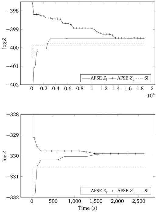
7. We prove the existence of a fully polynomial-time approximation scheme for the updating problem in credal networks of bounded treewidth over variables of bounded cardinality, and assuming strong independence. We show empirically that the approximation outperforms a state-of-the-art ap-proach for the problem. These results appeared in

Mauá, D. D., de Campos, C. P. and Zaffalon, M. [2011]. A fully polynomial time approximation scheme for updating credal networks of bounded treewidth and number of variable states,

Proceedings of the Seventh International Symposium on Imprecise Probability: Theories and Applications, pp. 277–286.

and

Mauá, D. D., de Campos, C. P. and Zaffalon, M. [2012]. Updat-ing credal networks is approximable in polynomial time,

Inter-national Journal of Approximate Reasoning 53(8): 1183–1199.

In order to keep the length of this dissertation reasonable, work on closely related subjects performed during the course of the author’s Ph.D. studies had to be omitted from this account, such as the evaluation of classifiers based on credal networks [Zaffalon et al., 2011, 2012], and the design of multilabel classifiers based on ensembles of Bayesian networks [Antonucci et al., 2013a].

1.2 Organization of the thesis

The rest of this document is organized in three chapters, each containing the results about one of the three classes of problems described. Chapter 2 contains the discussion on the problem of selecting maximum a posteriori configurations in discrete probabilistic graphical models. The complexity analysis of the strat-egy selection problem in limited memory influence diagrams is then presented in Chapter 3. The complexity results of updating credal networks are reported in Chapter 4. Finally, the overall conclusions of this work, together with directions on future work, are laid out in Chapter 5.

(20)

(21)

Chapter 2 Maximum a posteriori inference

Finding a mode of a probability distribution over a large number of discrete vari-ables, a task more commonly known as maximum a posteriori (MAP) inference, is a building block of many solutions to important applications such as image segmentation and categorization, 3D image reconstruction, natural language parsing, statistical machine translation, speech recognition, sentiment analysis, protein design, and multi-component fault diagnosis, to name but a few.

To allow for efficient manipulation and tractable inference, probability dis-tributions need to be concisely encoded. A class of models that achieves this goal is the class of probabilistic graphical models. These are multivariate models where irrelevance assessments between sets of variables are concisely described by means of a graph whose nodes are identified with variables [Pearl, 1988; Koller and Friedman, 2009]. Graphical models are usually distinguished accord-ing to whether their underlyaccord-ing graphical structure is directed. Bayesian

net-works are models in which a directed acyclic graph is used to represent a set of local Markov conditions: a variable is independent of the variables associated to

non-descendant non-parent nodes given the variables associated to its parents.

Markov random fields, on the other hand, encode independence assessments by

means of undirected graphs. In these models, the local Markov condition states that given (the variables associated to) its neighbors a variable is independent of its non-neighbors.

Although the type of graphical model chosen (i.e., directed or undirected) might greatly affect the complexity of specifying the requisite numerical param-eters of the model, it has little effect on the complexity of maximum a posteriori inference in discrete models. Indeed, by including new variables and/or setting some evidence, every Bayesian network can be efficiently transformed into an equivalent Markov network that assigns the same probability value for all

(22)

able assignments, and the converse is also true. Moreover, most algorithms can be applied equally to either class of graphical models. For these reasons, we shall not pursue the distinction between directed or undirected models in this chapter, and we shall adopt the language of factor graphs as a unifying visual representation of either type of model.

Probabilistic models often include latent variables, that is, variables that are not directly observable and yet are understood as important for modeling the phenomenon at hand. The inclusion of latent variables helps in eliciting the model from experts, and decreases the number of parameters required to cap-ture reasonably well the dependencies in the model, which can prevent over-fitting when learning models from data and lead to better results [Kwoh and Gillies, 1996; Binder et al., 1997; Friedman, 1998; Elidan et al., 2000; Zhang, 2004; Elidan and Friedman, 2005; Wang et al., 2013]. For instance, in determin-ing the premium of a car insurance application, the drivdetermin-ing skills and attitude of the applicant are important features which cannot be directly observed (by the analyst). Yet it is believed that these features strongly determine the likeli-hood of e.g. a driver being involved in a car accident and at the same time are strongly influenced by other personal factors such as the driver’s age [Binder et al., 1997]. Neglecting these features from the model drastically increases the number of parameters required to model the correlations between variables, which makes the model more difficult to specify and less effective [Friedman, 1998].

The problem of finding a mode of a discrete probabilistic graphical model is notoriously hard, and the presence of latent variables increases its computational complexity. For instance, the decision version of the MAP inference problem is NPPP_{-complete if the model contains (arbitrarily many) latent variables, while} the same problem is “only” NP-complete if latent variables make up a bounded fraction of the variables [Shimony, 1994; Park and Darwiche, 2004]. When the underlying graph is a tree, the problem with (arbitrarily many) latent variables is NP-complete [Park and Darwiche, 2004], whereas the same problem can be solved in polynomial time in the absence of latent variables [Koller and Fried-man, 2009]. Also finding a provably good approximation in trees of bounded degree is NP-hard in the presence of latent variables [Park and Darwiche, 2004] (however, a fully polynomial-time approximation scheme exists if the number of states per variable is assumed bounded, de Campos [2011]). Table 2.1 lists some of the known complexity results of the MAP inference problem in Bayesian networks (analogous results can be stated for Markov networks). Polytrees and loopy networks are defined in Chapter 3.

(23)

approxi-Table 2.1. Parametrized complexity of the MAP problem in Bayesian networks.

topology treewidth max. variable cardinality

complexity

“naive” tree one unbounded NP-complete

tree one five NP-complete

polytree two two NP-complete

polytree two unbounded NP-complete

loopy unbounded two NPPP_-complete

mate solutions. Recently, there has been a growing interest in the problem, with the development of many new approximate algorithms. Most of these algorithms provide solutions that can be arbitrarily poor, which might prevent the user of such algorithms from fully understanding the effects of approximate inference in the bigger picture of the application, that is, to know whether better results could be obtained by improving the quality of inference, or if it is the model or methodology that are fundamentally flawed. This is the case of message-passing and beam-search algorithms [Park and Darwiche, 2003; Dechter and Rish, 2003; de Campos et al., 2003; Yuan et al., 2004; Huang et al., 2006; Yuan and Hansen, 2009; Liu and Ihler, 2011; Jiang et al., 2011]. Such worries have very recently been addressed by Meek and Wexler [2011] and Cheng et al. [2012], who de-signed algorithms that are able to provide bounds within which the (probabil-ity of the) true solution is to be found.1 _{Moreover, these algorithms allow for} some trade-off between the tightness of the bounds and the amount of compu-tational resources (memory and time) used. Thus, loose bounds can justify an increase in processing time dedicated to inference if the final results turn out to be unsatisfactory, whereas tight bounds can reassure the quality of an efficient approximate inference algorithm. Moreover, bounds are necessary to account for alternative explanations in case conclusions are to be drawn from the result of the inference, as in scientific discovery (e.g., in finding associations between genes or proteins).

In the rest of this chapter, we briefly review some of the approaches to solve

1_{Some approximate methods such as the systematic search of Park and Darwiche [2003], the}

mini-bucket scheme of Dechter and Rish [2003] and the tree-reweighted variant of Liu and Ihler [2011] provide a “side guarantee”, that is, they are either inner or outer approximations. We can obtain an algorithm that provides bounds for the mode probability by combining an inner and an outer approximation algorithm.

(24)

the problem and present a new algorithm for the computation of MAP inferences in discrete graphical models of bounded treewidth (Section 2.2). The algorithm provides an assignment to the variables of interest and bounds on its posterior probability. In other words, the algorithm returns a solution and an estimate of its error relative to the optimal solution (i.e., the MAP assignment). The restric-tion to bounded treewidth models is necessary to enable efficient evaluarestric-tion of solutions, that is, to enable polynomial-time computation of the probability of a given assignment to the variables of interest. The algorithm is then extended into an anytime procedure, that is, an algorithm that is capable of monotonically improving the quality of its output as more time is granted (Section 2.3). We show asymptotic convergence and theoretical error bounds for any fixed number of steps of the algorithm. In Section 2.4, the performance of these algorithms is evaluated in experiments with real and synthetic models, and compared against the state-of-the-art systematic search algorithm of Park and Darwiche [2003]. Concluding remarks appear in Section 2.5.

Most of the content of this chapter is based on the work published in Refer-ence [Mauá and de Campos, 2012].

2.1 Graphical models and the MAP assignment problem

Consider a set X = {X1, . . . , Xn} of categorical variables, and an indexing set

S ⊆ [n] def= {1, . . . , n}. We call φ a factor if it is a mapping of the assignments

x_S def_{= {x}_i : i ∈ S} of a subset X_S_{= {X}_i : i ∈ S} of the variables into non-negative real numbers, in which case we call the corresponding variable-indexing set S its

scope. A (probabilistic) graphical model over X is a collection Φ = {φ1, . . . , φm}

of factors whose scopes S1, . . . , Smsatisfy S1∪· · · ∪ Sm=[n]. The model concisely

defines a probability measure on the sigma-field of subsets E of joint assignments xdef_{= {x}₁, . . . , x_n} to X by P(E)def=X x∈E 1 Z Y i∈[m] φi(xSi) , (2.1) where Z = Px Q

i∈[m]φi(xSi) is a normalizing constant known as the partition

function. We often write φ_i_{(x) to denote φ}_i_(x_S_i_{), leaving the domain implicit, if}

no ambiguity arises. If XS is a subset of variables, and xS a possible assignment of

values, the notations P(XS= xS) and P(xS) are used to denote the probability of

the event E = {x0_{: x}0

S = xS} induced by the joint assignments whose projection

(25)

φ1

φ₂ φ₃

φ4

X₁ X₂

X₃ X4

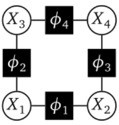
Figure 2.1. The factor graph of the graphical model in Example 2.1. The factor graph of a graphical model Φ is a bipartite graph whose nodes are identified either with factors φ in Φ or with variables Xi in X. The graph

contains an edge {φ, Xi} if i is in the scope of φ. The following example helps

in illustrating the concepts introduced thus far.

Example 2.1. Consider a graphical model Φ = {φ₁, φ₂, φ₃, φ₄} over four binary

variables X1, X2, X3 and X4, where the factors are specified by the tables below.

X₁ X₂ φ1(X1, X2) 0 0 10 1 0 0.1 0 1 0.1 1 1 10 X₁ X₃ φ2(X1, X3) 0 0 5 1 0 0.2 0 1 0.2 1 1 5 X2 X4 φ3(X2, X4) 0 0 5 1 0 0.2 0 1 0.2 1 1 5 X3 X4 φ4(X3, X4) 0 0 0.5 1 0 20 0 1 1 1 1 2.5

The corresponding factor graph is shown in Figure 2.1. The partition function is

Z = X

x1,x2,x3,x4

φ1(x1, x2)φ2(x1, x3)φ3(x2, x4)φ4(x3, x4) = 1224.384 ,

and P(X1=1, X2=1, X3=1, X4=1) = 10 · 5 · 5 · 2.5/Z = 0.5104607704.

We say that a variable Xi in X is a decision variable if its value is to be

deter-mined.2 _{The set D indexes the decision variables in X. The variables not indexed} 2_{The term “decision variable” can lead one to think that such a variable necessarily represents}

a quantity which can be controlled in the real world. This is however not the case, and such variables are often related to uncontrollable events.

(26)

by D are called latent variables, and are indexed by H (thus D ∪ H = [n] and

D ∩ H = ;). The MAP assignment problem consists in finding3

d∗∈ argmax d P(XD=d) = argmax d X x Y i∈[m] φi(x) Y j∈D δXj=dj(x) , (2.2) where δXj=dj def

= δ(xj− dj) denotes the Kronecker delta function that is one if

xj= dj, and zero otherwise. Note that in our terminology, δXj=dj is a factor with

scope {j}.

For any assignment ddef_{= {d}j : j ∈ D} to the decision variables, we can

inter-pret the argument of the maximization in (2.2), that is, the expression X x Y i∈[m] φi(x) Y j∈D δXj=dj(x) ,

as the probability measure defined by the augmented graphical model Φd =

Φ ∪S

j∈D{δXj=dj}. This probability measure assigns zero probability to joint

as-signments that are not consistent with d, and thus the partition function of the augmented model is Zd= P x Q i∈[m]φi(x) Q

j∈DδXj=dj(x). In other words, there

is a one-to-one correspondence between assignments d to the decision variables (which are the candidate solutions to the MAP assignment problem) and graph-ical models Φd=Φ ∪

S

j∈D{δXj=dj}, and the quality of each assignment d is given

by the partition function Zd of the corresponding graphical model Φd. This way,

we can re-state the MAP assignment problem as a search over graphical mod-els Φd instead of a search over assignments. Assume without loss of generality

that D = {1, . . . , k}, for some integer k < n, and H = {k + 1, . . . , n}, and define

K_i_={φ_i_{} for i = 1, . . . , m, and K}_j+m_={δ_X_j_=x_j : x_j _{∼ X}_i_{} for each decision j ∈ D.}4 Each combination of factors φ₁, . . . , φ_m+k from sets K₁, . . . , K_m+k, respectively, specifies the graphical model Φd corresponding to an assignment d to the

deci-sion variables. Let M = {{φ1, . . . , φm+k} : φi ∈ Ki} denote all graphical models

obtained in such a way. Finding a MAP assignment d∗ _{∈ argmax}

dP(XD= d) is

equivalent to finding a graphical model Φ∗_{∈ argmax} Φ∈M P x Q φ∈Φφ(x). An as-signment d∗_{= {d}∗

j : j ∈ D} is a MAP assignment if and only if there is a model

Φ∗ = {φ∗1, . . . , φm+k∗ } in M such that P x Q φ∈Φ∗φ(x) = max_Φ∈M P x Q φ∈Φφ(x) 3_{The formulation of the MAP assignment problem with delta functions is unusual, but it is}

important for the results and algorithm we devise later on.

4_{The notation x}

i∼ Xi denotes that xiis an element of the sample space of possible values of

(27)

and d∗_{= argmax}

d

Q

j∈Dφ∗j+k(dj) (or equivalently, if d∗j = argmaxdjφ

∗

j+k(dj) for

every j ∈ D).

Example 2.2. Consider the graphical model in Example 2.1, and suppose that D= {2, 3} and H ={1, 4}. The probability of each assignment to the decision variables

is shown in the table below. The rightmost column contains the unnormalized probabilities P0_(x 2, x3) = Z · P(x2, x3). X₂ X₃ _P(X₂, X3) P0(X2, X3) 0 0 0.11 135.054 1 0 0.2 251.25 0 1 0.01 12.75 1 1 0.67 825.33

Thus, {X2=1, X3=1} is the single MAP assignment.

To reformulate this MAP assignment problem as a search over graphical mod-els, consider the factors δX2=x2 and δX3=x3 for every MAP assignment {x2, x3}. Let

K₁ _{= {φ}₁_{}, K}₂ _{= {φ}₂_{}, K}₃ _{= {φ}₃_{}, K}₄ _{= {φ}₄_{}, K}₅ _{= {δ}_X₂₌₁, δX2=0} and K6 =

{δX3=1, δX3=0}. Each combination of factors ψ1, . . . , ψ6 ∈ K1, . . . , K6 corresponds

to the graphical model Φd induced by the assignment

d_=argmax

x1,x2

ψ5(x2)ψ6(x3) .

Let M be the family of all such graphical models Φd. An assignment {x∗₂, x₃∗} is a

MAP assignment if and only if there is model Φ∗

d= {ψ∗1, . . . , ψ∗6} in the set argmax Φ∈M X x1,x2,x3,x4 Y i∈[6] ψi(x) such that x∗ 2 = argmaxx2ψ ∗ 5(x2) and x3∗= argmaxx3ψ ∗ 6(x3). Hence, Φ∗={φ1, . . . , φ4, δX2=1, δX3=1}

is the solution equivalent to the MAP assignment {X2 = 1, X3 = 1}, and ZΦ∗ =

825.33.

2.2 Approximate algorithms for the MAP assignment

problem

In this section, we review some of the approaches to evaluation and selection of approximate MAP assignments, and present a new algorithm that provides bounds on the quality of the solution.

(28)

2.2.1 Clique-tree computation

We start by reviewing clique-tree algorithms, which can be used among other things to compute (not necessarily efficiently) MAP assignments in graphical models or to evaluate the unnormalized probability of a given assignment. Many algorithms use clique trees to organize data and schedule computations, and this is also the case for the algorithm we develop later on.

Clique-tree algorithms first appeared as methods to compute marginal prob-abilities in Bayesian networks [Lauritzen and Spiegelhalter, 1988; Shenoy and Shafer, 1988]. Motivated by the fact that computations in tree-shaped graphical models are usually efficient and straightforward [Pearl, 1988], clique-tree algo-rithms re-cast any graphical model as a tree. The efficiency of the computations in a clique tree is a function of the resemblance of the original graph to a tree.

Formally, let T be a tree over [m] such that each node i is associated to a set Ci ⊆ [n] and C1∪ · · · ∪ Cm= [n] for some positive integer n. We call T

a clique tree if for i = 1, . . . , n the sub-graph obtained by removing from T all nodes j such that i /_{∈ C}j remains connected.5 This condition is known as the

running intersection property, and guarantees that for any path in the tree (i.e.,

a sequence of non-repeating adjacent nodes) either an integer associated to the current node (i.e, some k ∈ Ci) appears for the last time in the path or it also

appears in the set associated to the adjacent node.

Let Φ be a graphical model whose factors φ1, . . . , φk have scopes S1, . . . , Sk,

respectively, and S₁_{∪ · · · ∪ S}_k_{=[n]. We say that (T, {C}₁, . . . , C_m_{}) is a clique tree} for Φ if T is a clique tree over [m], and for each i = 1, . . . , k there is j ∈ [m] such that Si ⊆ Cj. This last condition is called the family preserving property,

and it guarantees that the scope of each factor is covered by some set associated to a node of the clique tree, allowing us to associate each factor in the model to exactly one node in the clique tree. In the following, we assume for ease of exposition and without loss of generality that if T is a clique tree for Φ then

m = k and Si ⊆ Ci for all i, which allows us to unambiguously associate each

factor φ_i to the clique tree node i (for any C_i violating the assumption, we can include a new factor in Φ with domain XCi and image {1}; the running time of

the computations on the clique trees for both models have the same asymptotic growth rate, and the new graphical model induces the same probability mea-sure). This assumption is merely aesthetic, as it prevents us from dealing with

5_{In Chapter 3, we define the much similar concept of tree decomposition of a graph, which}

essentially refers to the same class of objects and could be used here instead. The distinction in terminology is that we see clique trees as objects not necessarily related to any graph, whereas the mention of a tree decomposition implies a reference graph.

(29)

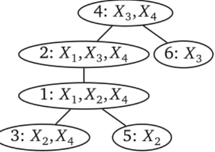
4: X₃, X₄ 2: X1, X3, X4 6: X3 1: X₁, X₂, X₄

3: X2, X4 5: X2

Figure 2.2. A clique tree for the family of graphical modelsM in Example 2.2. two indexing schemes (one for the factors and other for the nodes of the clique tree) and avoids the subsequent overcomplicated notation. The results obtained here do not depend, by any means, on that assumption.

The width of a clique tree is the cardinality of the largest set Ci minus one.

Since the complexity of algorithms that operate on clique trees is usually (at least) exponential in the tree width, one usually seeks to obtain a clique tree of low width. If it exists, a clique tree for a graphical model Φ of a given maximum width k (assumed constant) can be found in time linear in the scopes (but expo-nential in k) [Bodlaender, 1996]. In general, finding a minimum-width clique tree for a given graphical model is an NP-hard problem [Yannakakis, 1981], and one usually resorts to heuristics to obtain low-width trees, such as the minimum fill-in heuristic [Kjaerulff, 1990; van den Eijkhof et al., 2007].

Example 2.3. The tree in Figure 2.2 is a clique tree for any graphical model Φ_din

the family M in Example 2.2. The nodes 1, . . . , 4 are associated, respectively, with the factors φ₁, . . . , φ₄, whereas the nodes 5 and 6 are associated to factors δX2=x2

and δX3=x3, respectively, for some x2, x3. Note that S2 = {1, 3} ⊂ C2 = {1, 3, 4}.

The tree has width two, and one can show that there is no other suitable clique tree of smaller width.

The basic computation scheme with clique trees is the FACTOR-ELIMINATION

procedure in Algorithm 1, which computes the partition function of a graphical model Φ={φ1, . . . , φm} associated to a clique tree T over [m].6 Note that CPa(r)= ; in line 5. In a nutshell, the algorithm roots the tree in an arbitrary node (line 1), and then propagates messages containing the factors µi from the leaves

towards the root (lines 3–7). If r is the root node, we say that a node p of

6_{The algorithm is also known as the} _COLLECT _{algorithm [Shenoy and Shafer, 1988] and} JUNCTION-TREE PROPAGATIONalgorithm [Jensen and Nielsen, 2007], and is closely related to

vari-able elimination [Dechter, 1999], fusion in valuation algebras [Kohlas, 2003] and nonserial dynamic programming [Bertele and Brioschi, 1972].

(30)

Algorithm 1 FACTOR-ELIMINATION

Require: A clique tree T over a graphical model Φ = {φ1, . . . , φm}

Ensure: Z =P_XQ_i∈[m]φi

1: select a node r as root 2: label all nodes as inactive

3: whilethere is an inactive node i do

4: select an inactive node i with all children active

5: compute µ_i₌P X_Ci\CPa(i)φi Q j∈Ch(i)µj 6: label i as active 7: end while 8: Z =µ_r

the clique tree is the parent of a neighboring node i if p is closer to r. In this case, we also say that i is a child of p. The set of children and descendants of

i are denoted respectively by Ch(i) and De(i). Note that every node but the

root r has a single parent. The notation in line 5 representing the sum-marginal of a product of factors will be commonly used in the following discussion, and represents the factor µi over XCi∩CPa(i) such that

µi(x0) = X x∼X_Ci: x_Ci∩CPa(i)=x0 φi(xSi) Y j∈Ch(i) µj(xCi∩Cj) , (2.3) for all x0 _{∼ X}

Ci∩CPa(i). The propagation of messages halts when the root has

re-ceived one message from each child, in which case the partition function is ob-tained by Z = µr. The algorithm runs in O(msw+1) time, where s = maxi|{xi ∼

X_i_{}| is the maximum number of values a variable in the model can assume, and}

w = maxi|Ci| − 1 is the width of the clique tree. Thus when the width w is

bounded, the computations take polynomial time. Let h(i) def= S

j∈De(i)∪{i}Cj \ CPa(i) be the set of variable indexes that appear either in the set associated to node i or in any of its descendants. Due to the running intersection property, the factors containing only variables indexed by elements of h(i) are not involved in any computations performed in the loop of FACTOR-ELIMINATION after node i has been processed (i.e., after it has been

labeled as active). Consequently, it can be shown [Koller and Friedman, 2009] that for i = 1, . . . , m the factor µi satisfies

µi= X X_h(i) φi Y j∈De(i) φj. (2.4)

(31)

Since h(r)=[n] by definition of clique trees, the correctness of the computations follows from applying this result to the root: Z = µr =PX

Q

i∈[m]φi. Hence,

we can evaluate the quality of a candidate solution d to the MAP assignment problem by building a clique tree T for the corresponding graphical model Φd

and then running FACTOR-ELIMINATION, which produces Z_d₌P_XQ_φ_∈Φdφ. The

same clique tree structure can be used to evaluate different candidates.

Example 2.4. Consider the MAP problem in 2.2 and the clique tree T in Figure 2.2

as described in Example 2.3. We can evaluate the assignment d={X2=1, X3=0} by

running FACTOR-ELIMINATION with inputs T and Φ_d _{= {φ}₁, . . . , φ₄, δ_X

2=1, δX3=0} ,

which obtains Zd=

P

X1,X2,X3,X4

Q8

i=1φiδX2=1δX3=0 ∝ P(X2= 1, X2= 0). The same

clique tree could be used to evaluate e.g. the MAP assignment d={X2= 1, X3 = 1}

by running FACTOR-ELIMINATIONwith factors Φ_d_{= {φ}₁, . . . , φ₄, δ_X₂₌₁, δ_X₃₌₁}.

The algorithm can be straightforwardly modified to find a MAP assignment when there are no latent variables (i.e., when H =;) by substituting sums with maximizations in the computation of factors µ_i, obtaining aFACTOR-MAXIMIZATION

version of the algorithm in which µi= maxX_Ci\CPa(i)φi

Q

j∈Ch(i)µj (the correctness

of the procedure follows from the commutativity of maximization and product on the real numbers, Koller and Friedman [2009]). Indeed, a common approx-imation to MAP inference is to augment the decision set to D0_{= D ∪ H and run}

FACTOR-MAXIMIZATION, which then computes a lower bound on the value of

orig-inal MAP assignment problem. This idea naturally suggests a greedy approach to the computation of MAP assignments in the presence of latent variables (i.e.,

H 6= ;), which consists in redefining the factors µi so that latent variables are

summed out while decision variables are maximized. AFACTOR-MAX-ELIMINATION

version of the algorithm computes messages

µi=max X_Di X X_Hi φi Y j∈Ch(i) µj,

where D_i_=(C_i_{∩ D) \ C}_Pa(i)and H_i_=(C_i_{∩ H) \ C}_Pa(i). This approach has been pro-posed by Park and Darwiche [2003] as a cheap way of obtaining upper bounds on subsets of MAP assignments, which allows for a branch-and-bound proce-dure. Recently, iterative variants of this procedure that propagate messages in all directions until some convergence criteria is met have been proposed and justified as approximations by variational inference [Liu and Ihler, 2011; Jiang et al., 2011]. All these approaches retain the efficiency of message-passing al-gorithms for inference in graphical models, but produce only rough estimates to the real value. An exception is the use ofFACTOR-MAX-ELIMINATIONin a tree whose

(32)

root node r contains all decision variables. In this case, the procedure performs maximizations only after all latent variables have been marginalized out, which guarantees the correctness of the procedure for the MAP problem. Enforcing the clique tree to contain a node over all decision variables results in an exponential complexity in the number of decision variables [Park and Darwiche, 2004], un-less the factors in the root node are factorized [Meek and Wexler, 2011]. Thus, this approach is intractable in arbitrary large models. Yet, accuracy and runtime can be traded by “promoting” decision variables towards the root. Given any clique-tree rooted at r we promote a decision variable by including it in a node closer to the root (or in the root node itself), making sure that the running in-tersection property of tree decomposition is respected. Promoting variables can lead to tighter upper bounds, but also to a significant increase in running time [Park and Darwiche, 2004].

As mentioned in the previous paragraph, Park and Darwiche [2003] devel-oped a branch-and-bound procedure to the MAP assignment problem that sys-tematically searches over the space of assignments, running FACTOR-ELIMINATION

to evaluate each candidate solution,FACTOR-MAX-ELIMINATIONwith decision

vari-ables promoted until a given threshold on the width of the clique tree is achieved to obtain upper bounds on partial assignments. This strategy greatly narrows the search space, and makes the approach very competitive in practice. Their algo-rithm also allows for anytime inference, as the search can be stopped at any time returning the best solution found so far, and a better solution can be found with more time. We compare the algorithm we devise later on against theirs. Their algorithm has exponential worst-case running time, which is not surprising as the problem is NP-hard and can be reduced from SAT [Darwiche, 2009].

2.2.2 Propagating sets

Recall from the previous section that we can compare the quality of different can-didate solutions to the MAP assignment problem by running FACTOR-ELIMINATION

with the same clique tree but different indicator factors. More generally, con-sider a collection of sets of factors K1, . . . , Km such that all factors in each set

K_i have the same scope. Let Φ = {φ1, . . . , φm} be a graphical model obtained

by selecting one factor φi from each set Ki, i = 1, . . . , m, and let T be a clique

tree for this model. Then T is also a clique tree for any other graphical model induced by K1, . . . , Km. This is illustrated in the next example.

Example 2.5. Consider the sets of factors K₁, . . . , K₆ defined in Example 2.2, and

(33)

the node i in the clique tree. We also assign sets K₅ _{= {δ}_X₂_=x₂ : x₂ _{∼ X}₂_{} and}

K₆_{= {δ}X3=x3: x3∼ X3} to nodes 5 and 6, respectively, which makes T a clique tree

for all graphical models induced by these sets. Thus, the graphical models induced by the sets K₁, . . . , K6 are the graphical models Φd = {φ1, . . . , φ4, δX2=x2, δX3=x3}

in Example 2.3 that are in one-to-one correspondence with (unnormalized) prob-abilities of MAP assignments. Moreover, T is a suitable clique tree for any such model.

An arguably natural approach to approximately solve a MAP assignment problem, is to use some criteria to select a subset of candidate assignments, and evaluate the quality of each assignment in the subset runningFACTOR-ELIMINATION

on the same clique tree and the corresponding graphical model Φd. TheFACTOR

-SET-ELIMINATION procedure in Algorithm 2 implements such an approach, by

se-lecting assignments while it propagates sets of factors over the clique tree. The algorithm takes a clique tree T over a collection of sets of factors K₁, . . . , Km, and

a list of integers k1, . . . , km, and returns in time polynomial in the largest of those

integers a set of numbers that correspond to the (unnormalized) probabilities of a subset of the assignments, thus performing search and evaluation concurrently. The algorithm resembles FACTOR-ELIMINATION, but instead of propagating a

single message factor µ_i per node, it propagates sets of factors

L_i_{⊆ M}_i def₌    X X_Ci\CPa(i) φi Y j∈Ch(i) µj : φi ∈ Ki, µj∈ Lj    . (2.5)

As we shall see later on, the integer ki provided in the input determines the

maximum cardinality of the set L_i, and thus the worst-case time complexity of the algorithm. A larger value of ki allows more factors to be propagated at node

i, which increases the computational burden and potentially the accuracy of the

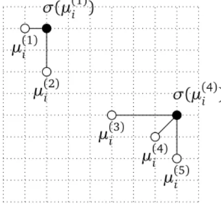
algorithm. The object σ first referred to in line 1 is a function from message factors µ_i into factors σ(µi), where the latter accounts for errors introduced

when discarding elements from Mi so as to keep the cardinality of Li within the

given bound ki. We shall discuss later on how the elements σ(µi) in lines 6

and 16 are obtained. The pruning operations in lines 8 and 18 return a subset

L_i _{⊆ M}_i of cardinality k_i and recompute the upper bounds σ(µi) to account for

the discarded elements. So, if ki ≥ |Mi|, the pruning operation returns Li= Mi.

The algorithm outputs lower and upper bounds Zl and Zu, respectively, to the

maximum partition function Z∗_{= max{}P

X

Q

i∈[m]φi : φi ∈ Ki} of a graphical

(34)

corre-Algorithm 2 FACTOR-SET-ELIMINATION

Require: A clique tree T over the sets of factors K₁, . . . , K_m and positive integers

k₁, . . . , k_m

Ensure: Zl ≤ Z∗≤ Zu

1: select a node r as root and let σ be an empty dictionary 2: for allleaf node i do

3: let M_i be an empty set 4: for allφi∈ Ki do 5: add µ_i ₌P X_Ci\CPa(i)φi to Mi 6: _{set σ(µ}_i_{) ← µ}_i 7: end for 8: L_i _{= prune(M}_i, σ_i, k_i₎ 9: end for

10: label leaves as active and internal nodes as inactive

11: whilethere is an inactive node do

12: select an inactive node i whose children are all active 13: let M_i be an empty set

14: for allφi∈ Ki, µj ∈ Lj, j ∈ Ch(i) do

15: add µ_i ₌P X_Ci\CPa(i)φi Q j∈Ch(i)µj to Mi 16: set σ(µ_i_{) ←}P X_Ci\CPa(i)φi Q j∈Ch(i)σ(µj) 17: end for 18: L_i _{= prune(M}_i, σ, k_i₎ 19: label i as active 20: end while 21: Z_l _{= max{µ}_r: µr ∈ Lr} 22: Z_u_{= max{σ(µ}_r_{) : µ}_r_{∈ L}_r_}

spondence of factors µi ∈ Li computed by this algorithm to those computed with

FACTOR-ELIMINATION.

Theorem 2.1. For i = 1, . . . , m, any µi ∈ Li satisfies µi=PX_h(i)φi

Q

j∈De(i)φj for

some combination of φ_i_{∈ K}_i and φ_j _{∈ K}_j _{for all j ∈ De(i).}

Proof. First, note that the definition of µ_i in FACTOR-SET-ELIMINATION is identical

to the definition in FACTOR-ELIMINATION. Assume the pruning operations are not

performed, that is, that prune(Mi, σi, ki) returns Mi. Then it is not difficult to

see that µi matches the computation in FACTOR-ELIMINATION for some graphical

model induced by K1, . . . , Km. But since the pruning operation returns a subset

(35)

The following result follows immediately from the above theorem.

Corollary 2.1. Z_l₌P_XQ_i∈[m]φi for some combination of factors (φ1, . . . , φm) ∈

K₁_{× · · · × K}_m.

If the algorithm is run with factor sets K1, . . . , Km that induce graphical

mod-els corresponding to different assignments to decision variables as explained in Section 2.1, the numbers Z_l and Z_u returned are lower and upper bounds for the MAP assignment probability Z∗_{= max}

dP(XD= d). In fact, if ki= |Mi| for all

i = 1, . . . , m, the algorithm is equivalent to an exhaustive search over the space

of assignments, and thus returns Zl= Z∗. Moreover, the value of Zl is actually

achieved by some assignment, and hence denotes the value of a feasible solu-tion. The assignment corresponding to Zl can be obtained by tracking back the

indicator factors δi, i ∈ D that were propagated to generate the number µr= Zl,

as in the following example.

Example 2.6. Consider the sets of factors K1, . . . , K6 in Example 2.5, and the clique

tree T in Figure 2.2. Let us simulate a run of FACTOR-SET-ELIMINATION on inputs

K₁, . . . , K₆, T and k₁, . . . , k₆, with integers k_i set to some sufficiently high value so

that no pruning takes effect (i.e., Li = Mi for all i). This also makes the upper

bounds tight, that is, σ(µi) = µi for any µi in Mi and Li, i = 1, . . . , 6.

First, for i = 1, . . . , 6, we associate to each node i the set Ki. Suppose node 4 is

selected as root. Then, 3,5 and 6 are leaf nodes, while 1 and 2 are internal nodes. The first loop of the algorithm processes all the leaf nodes, obtaining the sets

M₃_{= {φ}₃_{} , M}₅ _{= {φ}₅: φ5∈ K5} = {δX2=1, δX2=0} ,

M6= {φ6: φ6∈ K3} = {δX3=1, δX3=0} .

The second loop processes the remaining nodes. In the first iteration of the loop, the algorithm selects node 1 (as it is the only being inactive and having all children active at this stage), and computes

M₁₌ ( X X2 φ₁µ₂µ₃: µ₂ _{∈ L}₂, µ₃_{∈ L}₃ ) = ( X X2 φ₁φ₃δ_X₂₌₁,X X2 φ₁φ₃δ_X₂₌₀ ) .

Next, the algorithm selects node 2 and computes

M₂₌ ( X X1 φ1µ1: µ1∈ L1 ) = ( X X1 φ2 X X2 φ1φ3δX2=1, X X2 φ1φ3δX2=0 ) .

(36)

Finally, node 4 is selected, which causes the computation of M₄₌ ( X X3,X4 φ₄µ₂µ₃: µ₂_{∈ L}₂, µ₃_{∈ L}₃ ) = ¨ X X3,X4 φ4 X X1 φ2 X X2 φ1φ3δX2=1 ! δX3=1, X X3,X4 φ4 X X1 φ2 X X2 φ1φ3δX2=0 ! δX3=1, X X3,X4 φ4 X X1 φ2 X X2 φ1φ3δX2=1 ! δX3=0, X X3,X4 φ4 X X1 φ2 X X2 φ1φ3δX2=0 ! δX3=0 « .

The algorithm returns the highest of the numbers {µ4 : µ4 ∈ L4}, which according

to Corollary 2.1 and the computations in Example 2.2 is Zl = X X1,X2,X3,X4 Y i∈[4] φ1δX2=1δX3=1= 825.33 .

The MAP assignment can be obtained by labeling each factor with corresponding decision variable assignments (or an empty character if the factor does not corre-spond to a partial assignment of decision variables). To this end, label each factor φi in Ki, i = 1, . . . , 4 with an empty string, and label each factor δXi=xi in Ki, i = 5, 6, with the string “(Xi = xi)”. Then, label each µi in Mi, i = 1, . . . , 6 with

the concatenation of the labels of its constituting factors. An inductive argument suffices to show that e.g. the label of µ(1)

1 = P X2φ1φ2δX2=1 is “(X2= 1)”, the label of µ(2) 2 = P X1φ2 P

X2φ1φ3δX2=0 is “(X2= 0)”, and the label of Zl=max{µ4: µ4∈

L₄_{} is “(X}₂_{= 1)(X}₃_{= 1)”.}

Note that since no “pruning” was performed, the algorithm in the last step maximizes over as many numbers as assignments of decision variables, which is equivalent to an exhaustive search.

The complexity of the algorithm is determined by the number of additions and multiplications needed to compute each factor µi in a set Mi plus the

com-plexity of the pruning operation (which we describe in detail later on). Analo-gously toFACTOR-ELIMINATION, the complexity of computing each µ_i is O(msw+1_).

(37)

contains |Ki|

Q

j∈Ch(i)|Lj| = |Ki|

Q

j∈Ch(i)kj ≤ kc elements, where c is the

maxi-mum number of neighbors of a node. Hence, the algorithm runs in O(kc_msw

). If the clique tree given as input contains a bounded number of neighbors for each node and bounded width, the algorithm runs in time polynomial in the inputs

k₁, . . . , k_m and K₁, . . . , K_m. Note that for any given graphical model of bounded treewidth we can obtain a suitable clique tree of bounded width and bounded number of neighbors per node (e.g., a binary clique tree, Shenoy [1997]).

2.2.3 Pruning messages

As in Example 2.6, without any pruning operation, the FACTOR-SET-ELIMINATION

algorithm amounts to an efficient enumerative scheme, that evaluates all possi-ble solutions while avoiding many redundant computations that would be per-formed by runningFACTOR-ELIMINATIONon each solution. As such, the algorithm

is not applicable to any reasonably large problem. Thus, the algorithm’s effi-ciency heavily depends on the pruning operations, which are responsible for limiting the cardinality of the propagated sets according to the input parame-ters k1, . . . , km. In the following, we discuss how to derive pruning operations

that allow for a trade-off between the quality of the solutions obtained and the computation time as determined by those input parameters.

Pruning by convexification

Consider a set of factors M_i produced duringFACTOR-SET-ELIMINATION which we

wish to prune to produce a smaller set Li whose cardinality is not greater than

the allowed cardinality ki. A factor µ(1)i in Mi is a convex combination of factors

µ(2)_i and µ(3)_i if there is a real 0 ≤ λ ≤ 1 such that µ(1)_i = λµ(2)i + (1 − λ)µ(3)i . A

factor µ_i _{∈ M}_i is an extreme if it is not a convex combination of any two other elements in the set (extremes or not). As the following result shows, convex combinations can be safely discarded from the propagation, as they certainly are outperformed by some extrema.

Proposition 2.1. Let µ(1)_i , µ(2)_i and µ(3)_i be three different factors in a set M_i such

that µ(1)

i is a convex combination of µ(2)i and µ(3)i . Let also µ(1)r be a solution

obtained by propagating µ(1)

i up to the root. Then, there is a solution µr obtained

by propagating either µ(2)

i or µ(3)i up to the root that satisfies µ(1)r < µr.

Proof. Let µ(1) j = P X_{C j\Cp} φjµ(1)i Q k∈Ch(j)\{i}µk, µ(2)j = P X_{C j\Cp} φjµ(2)i Q k∈Ch(j)\{i}µk and µ(3) j = P X_{C j\Cp}φjµ(3)i Q