USING CONSTRAINT SATISFACTION TECHNIQUES AND VARIATIONAL METHODS FOR PROBABILISTIC REASONING
MOHAMED IBRAHIM
DÉPARTEMENT DE GÉNIE INFORMATIQUE ET GÉNIE LOGICIEL ÉCOLE POLYTECHNIQUE DE MONTRÉAL
THÈSE PRÉSENTÉE EN VUE DE L’OBTENTION DU DIPLÔME DE PHILOSOPHIÆ DOCTOR
(GÉNIE INFORMATIQUE) AOÛT 2015
c
ÉCOLE POLYTECHNIQUE DE MONTRÉAL
Cette thèse intitulée:
USING CONSTRAINT SATISFACTION TECHNIQUES AND VARIATIONAL METHODS FOR PROBABILISTIC REASONING
présentée par: IBRAHIM Mohamed
en vue de l’obtention du diplôme de: Philosophiæ Doctor a été dûment acceptée par le jury d’examen constitué de:
M. MULLINS John, Ph. D., président
M. PESANT Gilles, Ph. D., membre et directeur de recherche M. PAL Christopher J., Ph. D., membre et codirecteur de recherche M. DESMARAIS Michel C., Ph. D., membre
DEDICATION
To my beloved mother, the memory of my father and to my lovely wife and children, with endless love and gratitude
ACKNOWLEDGEMENTS
First and foremost, I sincerely offer praise to ALLAH for providing me the health, patience, and knowledge to complete my thesis.
I would like to express my deepest gratitude to my supervisors, Prof. Gilles Pesant and Prof. Christopher Pal, whose expertise, understanding, and patience, added considerably to my graduate experience. I am grateful for everything I learned from them, for their continuous support throughout my study and research, and for providing me with invaluable insights which helped me solve many of the problems I encountered in my research. It was simply impossible producing this thesis without their excellent guidance.
I would like to take this as an opportunity to thank Prof. John Mullins, Prof. Michel Des-marais, and Prof. Peter Van Beek for assigning part of their time to review this dissertation and to serve on my thesis committee.
I would like to acknowledge the Ministry of Higher Education, Egypt and my supervisors for respectively supporting me financially during my Ph.D. which gave me opportunities to complete this thesis.
I also thank all my colleagues, friends, and all the selfless and active workers serving society as well.
Last but certainly not least, I am very thankful to my family: To my mother, Hameeda Ali-Eldin, who somehow convinced me that ‘failure’ is not a dictionary word; to my father, Hamza Ibrahim to whom I never managed to explain what I do but who is always happy for my success, my sister, Marwa Ibrahim, my wife, Zolfa Selmi, and my children, Youssef, Seif and Habiba for their support and encouragement. I love you all so much!
RÉSUMÉ
Cette thèse présente un certain nombre de contributions à la recherche pour la création de systèmes efficaces de raisonnement probabiliste sur les modèles graphiques de problèmes issus d’une variété d’applications scientifiques et d’ingénierie. Ce thème touche plusieurs sous-disciplines de l’intelligence artificielle. Généralement, la plupart de ces problèmes ont des modèles graphiques expressifs qui se traduisent par de grands réseaux impliquant déter-minisme et des cycles, ce qui représente souvent un goulot d’étranglement pour tout système d’inférence probabiliste et affaiblit son exactitude ainsi que son évolutivité.
Conceptuellement, notre recherche confirme les hypothèses suivantes. D’abord, les tech-niques de satisfaction de contraintes et méthodes variationnelles peuvent être exploitées pour obtenir des algorithmes précis et évolutifs pour l’inférence probabiliste en présence de cycles et de déterminisme. Deuxièmement, certaines parties intrinsèques de la structure du modèle graphique peuvent se révéler bénéfiques pour l’inférence probabiliste sur les grands modèles graphiques, au lieu de poser un défi important pour elle. Troisièmement, le re-paramétrage du modèle graphique permet d’ajouter à sa structure des caractéristiques puissantes qu’on peut utiliser pour améliorer l’inférence probabiliste.
La première contribution majeure de cette thèse est la formulation d’une nouvelle approche de passage de messages (message-passing) pour inférer dans un graphe de facteurs étendu qui combine des techniques de satisfaction de contraintes et des méthodes variationnelles. Contrairement au message-passing standard, il formule sa structure sous forme d’étapes de maximisation de l’espérance variationnelle. Ainsi, on a de nouvelles règles de mise à jour des marginaux qui augmentent une borne inférieure à chaque mise à jour de manière à éviter le dépassement d’un point fixe. De plus, lors de l’étape d’espérance, nous mettons à profit les structures locales dans le graphe de facteurs en utilisant la cohérence d’arc généralisée pour effectuer une approximation de champ moyen variationnel.
La deuxième contribution majeure est la formulation d’une stratégie en deux étapes qui utilise le déterminisme présent dans la structure du modèle graphique pour améliorer l’évolutivité du problème d’inférence probabiliste. Dans cette stratégie, nous prenons en compte le fait que si le modèle sous-jacent implique des contraintes inviolables en plus des préférences, alors c’est potentiellement un gaspillage d’allouer de la mémoire pour toutes les contraintes à l’avance lors de l’exécution de l’inférence. Pour éviter cela, nous commençons par la relaxation des préférences et effectuons l’inférence uniquement avec les contraintes inviolables. Cela permet d’éviter les calculs inutiles impliquant les préférences et de réduire la taille effective du réseau
graphique.
Enfin, nous développons une nouvelle famille d’algorithmes d’inférence par le passage de mes-sages dans un graphe de facteurs étendus, paramétrées par un facteur de lissage (smoothing parameter). Cette famille permet d’identifier les épines dorsales (backbones) d’une grappe qui contient des solutions potentiellement optimales. Ces épines dorsales ne sont pas seulement des parties des solutions optimales, mais elles peuvent également être exploitées pour inten-sifier l’inférence MAP en les fixant de manière itérative afin de réduire les parties complexes jusqu’à ce que le réseau se réduise à un seul qui peut être résolu avec précision en utilisant une méthode MAP d’inférence classique. Nous décrivons ensuite des variantes paresseuses de cette famille d’algorithmes.
Expérimentalement, une évaluation empirique approfondie utilisant des applications du monde réel démontre la précision, la convergence et l’évolutivité de l’ensemble de nos algorithmes et stratégies par rapport aux algorithmes d’inférence existants de l’état de l’art.
ABSTRACT
This thesis presents a number of research contributions pertaining to the theme of creating ef-ficient probabilistic reasoning systems based on graphical models of real-world problems from relational domains. These models arise in a variety of scientific and engineering applications. Thus, the theme impacts several sub-disciplines of Artificial Intelligence. Commonly, most of these problems have expressive graphical models that translate into large probabilistic networks involving determinism and cycles. Such graphical models frequently represent a bottleneck for any probabilistic inference system and weaken its accuracy and scalability. Conceptually, our research here hypothesizes and confirms that: First, constraint satisfaction techniques and variational methods can be exploited to yield accurate and scalable algorithms for probabilistic inference in the presence of cycles and determinism. Second, some intrinsic parts of the structure of the graphical model can turn out to be beneficial to probabilistic inference on large networks, instead of posing a significant challenge to it. Third, the proper re-parameterization of the graphical model can provide its structure with characteristics that we can use to improve probabilistic inference.
The first major contribution of this thesis is the formulation of a novel message-passing approach to inference in an extended factor graph that combines constraint satisfaction tech-niques with variational methods. In contrast to standard message-passing, it formulates the Message-Passing structure as steps of variational expectation maximization. Thus it has new marginal update rules that increase a lower bound at each marginal update in a way that avoids overshooting a fixed point. Moreover, in its expectation step, we leverage the local structures in the factor graph by using generalized arc consistency to perform a variational mean-field approximation.
The second major contribution is the formulation of a novel two-stage strategy that uses the determinism present in the graphical model’s structure to improve the scalability of probabilistic inference. In this strategy, we take into account the fact that if the underlying model involves mandatory constraints as well as preferences then it is potentially wasteful to allocate memory for all constraints in advance when performing inference. To avoid this, we start by relaxing preferences and performing inference with hard constraints only. This helps avoid irrelevant computations involving preferences, and reduces the effective size of the graphical network.
Finally, we develop a novel family of message-passing algorithms for inference in an extended factor graph, parameterized by a smoothing parameter. This family allows one to find the
“backbones” of a cluster that involves potentially optimal solutions. The cluster’s backbones are not only portions of the optimal solutions, but they also can be exploited for scaling MAP inference by iteratively fixing them to reduce the complex parts until the network is simplified into one that can be solved accurately using any conventional MAP inference method. We then describe lazy variants of this family of algorithms. One limiting case of our approach corresponds to lazy survey propagation, which in itself is novel method which can yield state of the art performance.
We provide a thorough empirical evaluation using real-world applications. Our experiments demonstrate improvements to the accuracy, convergence and scalability of all our proposed algorithms and strategies over existing state-of-the-art inference algorithms.
TABLE OF CONTENTS DEDICATION . . . iii ACKNOWLEDGEMENTS . . . iv RÉSUMÉ . . . v ABSTRACT . . . vii TABLE OF CONTENTS . . . ix
LIST OF TABLES . . . xiii
LIST OF FIGURES . . . xiv
LIST OF SYMBOLS AND ABBREVIATIONS . . . xviii
LIST OF APPENDICES . . . xix
CHAPTER 1 INTRODUCTION . . . 1
1.1 Overview and Motivations . . . 1
1.2 Problem Statement and Limitations . . . 1
1.2.1 Problem 1 . . . 2
1.2.2 Problem 2 . . . 4
1.2.3 Problem 3 . . . 4
1.3 Research Questions and Objectives . . . 6
1.4 Summary of the Contributions . . . 7
1.5 Organization of the Dissertation . . . 9
CHAPTER 2 BACKGROUND . . . 11
2.1 Basic Notation and Definitions . . . 11
2.2 Probabilistic Graphical Models . . . 14
2.2.1 Ising Models . . . 15
2.2.2 Markov Logic Networks . . . 16
2.2.3 Factor Graphs . . . 17
2.3 Probabilistic Reasoning over Graphical Models . . . 19
2.3.2 Markov Chain Monte Carlo Methods . . . 22
2.3.3 Local Search Methods . . . 23
2.4 Constraint Satisfaction Techniques for Analyzing Constraint Problems . . . . 25
2.4.1 Constraint Satisfaction Problems . . . 25
2.4.2 Clustering Phenomenon and Geometry of the Solution Space . . . 27
2.4.3 The Survey Propagation Model of Satisfiability . . . 29
2.4.4 Decimation Based on Survey Propagation . . . 30
2.5 Variational Approximation Methods . . . 31
2.5.1 Variational Expectation Maximization . . . 31
2.5.2 Variational Mean Field approximation . . . 32
CHAPTER 3 LITERATURE REVIEW . . . 33
3.1 Message-Passing Techniques for Computing Marginals . . . 33
3.1.1 Studying Message-passing’s convergence . . . 33
3.1.2 Damped Message-passing . . . 35
3.1.3 Re-parameterized Message-passing . . . 35
3.1.4 Message passing and variational methods . . . 35
3.1.5 Scalable Message Passing . . . 36
3.2 Integrating Constraint Satisfaction techniques with Message Passing . . . 37
3.2.1 Constraint Propagation Based Methods . . . 37
3.2.2 Survey Propagation Based Methods . . . 38
3.3 Solving Maximum-A-Posteriori Inference Problems . . . 38
3.3.1 Systematic and Non-Systematic Search Methods . . . 39
3.3.2 Message-Passing-Based Methods . . . 40
3.3.3 Scalable MAP Methods . . . 41
CHAPTER 4 IMPROVING INFERENCE IN THE PRESENCE OF DETERMINISM AND CYCLES . . . 42
4.1 GEM-MP Framework . . . 42
4.2 GEM-MP General Update Rule for Markov Logic . . . 56
4.2.1 Hard-update-rule . . . 57
4.2.2 Soft-update-rule. . . 64
4.3 GEM-MP versus LBP . . . 68
4.4 GEM-MP Algorithm . . . 69
4.5 GEM-MP Update Rules for Ising MRFs . . . 70
4.6 Experimental Evaluation . . . 71
4.6.2 Metrics . . . 74
4.6.3 Methodology and Results . . . 75
4.7 Discussion . . . 91
CHAPTER 5 EXPLOITING DETERMINISM TO SCALE INFERENCE . . . 95
5.1 Scaling Up Relational Inference via PR . . . 95
5.1.1 The PR Framework . . . 96
5.2 PR-based Relational Inference Algorithms . . . 98
5.2.1 PR-BP . . . 98
5.2.2 PR-MC-SAT . . . 99
5.3 Combining PR with Lazy Inference . . . 99
5.4 Experimental Evaluations . . . 100 5.4.1 Metrics . . . 101 5.4.2 Methodology . . . 101 5.4.3 Datasets . . . 102 5.4.4 Results . . . 103 5.5 Discussion . . . 111
CHAPTER 6 IMPROVING MAP INFERENCE USING CLUSTER BACKBONES 113 6.1 WSP-χ Framework . . . . 113
6.1.1 Factor Graph Re-parameterization . . . 113
6.1.2 WSP-χ Message-Passing . . . . 117
6.1.3 A Family of Extended Factor Graphs . . . 118
6.1.4 Derivation of WSP-χ’s Update Equations . . . . 120
6.2 Using WSP-χ for MAP Inference in Markov Logic . . . . 126
6.3 Combining WSP-χ with Lazy MAP Inference . . . 129
6.4 Experimental Evaluation . . . 129
6.4.1 Methodology . . . 131
6.4.2 Metrics . . . 132
6.4.3 Results . . . 132
6.5 Discussion . . . 146
CHAPTER 7 CONCLUSION AND FUTURE WORK . . . 148
7.1 GEM-MP Inference Approach . . . 148
7.2 Preference Relaxation Scaling Strategy . . . 149
7.3 WSP-χ Family of Algorithms . . . 149
7.5 Future Work . . . 150 REFERENCES . . . 153 APPENDICES . . . 167
LIST OF TABLES
Table 2.1 An excerpt of the knowledge base for the Cora dataset. The atoms SameBib and SameAuthor are unknown. Ar() is an abbreviation for atom Author(), SAr() for SameAuthor(), and SBib() for SameBib(). a1, a2 represent authors and r1, r2, r3 represent citations. . . 11
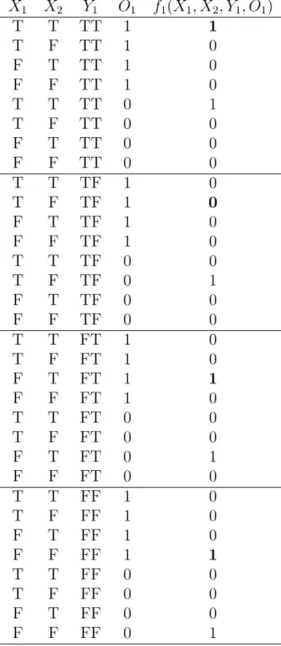
Table 4.1 Factor f1 in the original factor graph (left). Its corresponding extended
factor ˆf1 in the extended factor graph (right). When the activation
node O1 = 1, the bold values are cases in which the extended factor ˆf1
preserves the same value of f1. Otherwise it assigns a value 0. When
the activation node O1 6= 1, the matches between Y1 and (X1, X2) are
cases in which ˆf1 assigns a value 1. Otherwise it assigns a value 0. . . 46
Table 4.2 General update rules of GEM-MP inference for Markov logic. These rules capture relationships between ground atoms with each other, and therefore it does not necessitate explicitly passing messages between atoms and clauses. . . 67 Table 4.3 Average F1 scores for the GEM-MP, MC-SAT, Gibbs, LBP, LMCSAT,
and L-Im inference algorithms on Cora, Yeast, and UW-CSE at the end of the allotted time. . . 79 Table 5.1 Average Construction (with and without PR) and Inference times (mins.),
memory (MB) and accuracy (CLL) metrics of Propositional grounding and PR-based MC-SAT inference algorithms on the Yeast data set over 200 objects, the UW-CSE data set over 150 objects, and the Cora data set over 200 objects. . . 112 Table 6.1 (Left) The joint probabilities of complete assignments {1, 0, 1} and
{1, 1, 1} in the original factor graph. (Right) The (solution cluster-based) joint probabilities of their corresponding configurations ρX in the extended factor graph, where ˆwc(resp. ˆwd) are the weights
associ-ated with the factors fc (resp. fd) that are satisfied by the underlying
complete assignments. . . 117 Table 6.2 The percentage of the frozen ground atoms (i.e., cluster backbones)
that are fixed (fixed%) and the average cost of unsatisfied clauses (Cost) for a family of WSP-Dec at different choices of smoothing pairs (χ,γ) on Cora, Web-KB, and Yeast. The cooling parameter y assigned a value 2 and the threshold takes a value 0.2. . . . 145
LIST OF FIGURES
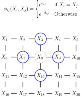
Figure 1.1 A preliminary experiment illustrates the effects of cycles and deter-minism on the convergence behaviour of LBP in Cora dataset (Singla and Domingos, 2006a) (left) and Yeast dataset (Singla and Domingos, 2006a) (right). These datasets and their models are publicly available at the alchemy website: http://alchemy.cs.washington.edu/data/ . . . 3 Figure 2.1 A 2D lattice represented as undirected graphical model. The red node
X8 is independent of the other black nodes given its neighbors (blue
nodes) . . . 15 Figure 2.2 Grounded factor graph obtained by applying clauses in Table 2.1 to
the constants: {Gilles(G), Chris(C)} for a1 and a2; {C1, C2} for r1,
r2, and r3. The factor graph involves: 12 ground atoms in which 4
are evidence (dark ovals) and 8 are non-evidence (non-dark ovals); 24 ground clauses wherein 8 are hard (Fh = {f
1, · · · , f8}) and 16 are soft
(Fs= {f
9, · · · , f24}). . . 18
Figure 2.3 A depiction of the LBP’s message-passing process on a simple factor graph consists of four variables {X1, . . . , X4} and four factors {f1, . . . , f4}.
It shows how LBP passes two types of messages: from variables to fac-tors (in red) and from facfac-tors to variables (in blue). . . 21 Figure 2.4 A notional depiction of the clustering phenomenon. It shows how the
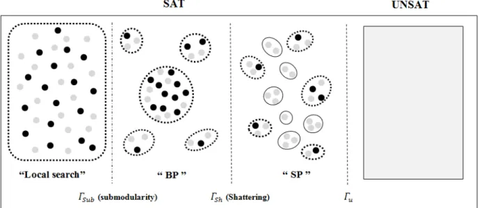
space between solutions varies as Γ increases. Solutions are depicted as solid circles, while unsatisfying assignment or near-solution (which satisfy almost all, but not all, of the clauses) appear as fainter circles. Within the limitations of a two-dimensional representation, the place-ment of assignplace-ments represents their Hamming distances. Thus, two assignments are considered adjacent if they have very small Hamming distance (e.g., they differ by a single variable). In addition, dotted outlines group adjacent assignments into arbitrary clusters of interest, while solid outlines group assignments into metastable clusters (Kilby et al., 2005; Chavas et al., 2005), which have no solutions. Finally, un-der each phase transition of the solution space, the solving technique that is widely used in the literature to find a solution relatively quickly, is indicated. . . 28
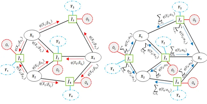
Figure 4.1 An example factor graph G (left) which is a fragment of the Cora example in Figure 2.2, that involves factors F = {f1, f2, f3, f4} and
three random variables {X1, X2, X3} representing query ground atoms
{SBib(C2, C2), SBib(C2, C1), SBib(C1, C2)}. The extended factor graph
ˆ
G (right) which is a transformation of the original factor graph after adding auxiliary mega-node variables Y = {y1, y2, y3, y4}, and auxiliary
activation-node variables O = {O1, O2, O3, O4}, which yields extended
factors ˆF = nfˆ1, ˆf2, ˆf3, ˆf4
o
. . . 43
Figure 4.2 Illustrating message-passing process of GEM-MP. (left) Eq(X )-step mes-sages from variables-to-factors; (right) Eq(Y)-step messages from factors-to-variables. . . 52
Figure 4.3 Illustrating how each step of the GEM-MP algorithm is guaranteed to increase the lower bound on the log marginal-likelihood. In its “Mq(Y) -step”, the variational distribution over hidden mega-node variables is maximized according to Eq. (4.15). Then, in its “Mq(X )-step”, the variational distribution over hidden X variables is maximized according to Eq. (4.16). . . 55
Figure 4.4 Average CLL as a function of inference time for GEM-MP, MC-SAT, LBP, Gibbs, LMCSAT, and L-Im algorithms on Cora. . . 76
Figure 4.5 Average CLL as a function of inference time for GEM-MP, MC-SAT, LBP, Gibbs, LMCSAT, and L-Im algorithms on Yeast. . . 77
Figure 4.6 Average CLL as a function of inference time for GEM-MP, MC-SAT, LBP, Gibbs, LMCSAT, and L-Im algorithms on UW-CSE. . . 78
Figure 4.7 The impact of gradual zones of determinism on the accuracy of GEM-MP, MC-SAT and LBP algorithms for Cora dataset. . . 81
Figure 4.8 The impact of gradual zones of determinism on the accuracy of GEM-MP, MC-SAT and LBP algorithms for Yeast dataset. . . 82
Figure 4.9 The impact of gradual zones of determinism on the accuracy of GEM-MP, MC-SAT and LBP algorithms for UW-CSE dataset. . . 83
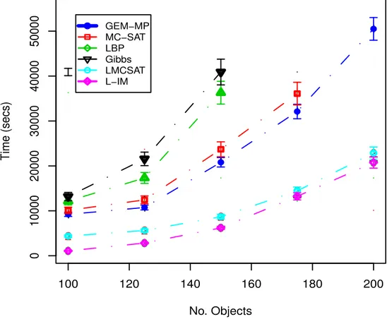
Figure 4.10 Inference time vs. number of objects in Cora. . . 84
Figure 4.11 Inference time vs. number of objects in Yeast. . . 85
Figure 4.12 Inference time vs. number of objects in UW-CSE. . . 86
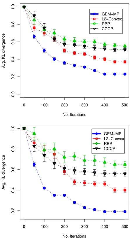
Figure 4.13 The results of 20 × 20 grids of Ising model: The cumulative percentage of convergence (Convergence %) vs. number of iterations at determin-ism Zone1 [0% − 20%] (Top) and at determindetermin-ism Zone2 [20% − 40%] (Bottom). . . . 89
Figure 4.14 The results of 20 × 20 grids of Ising model: The average KL-divergence (KL) metric vs. number of iterations at determinism Zone1 [0% − 20%] (Top) and at determinism Zone2 [20% − 40%] (Bottom). . . . 90 Figure 4.15 From Top to middle: The average CLL of GEM-MP-random (x-axis)
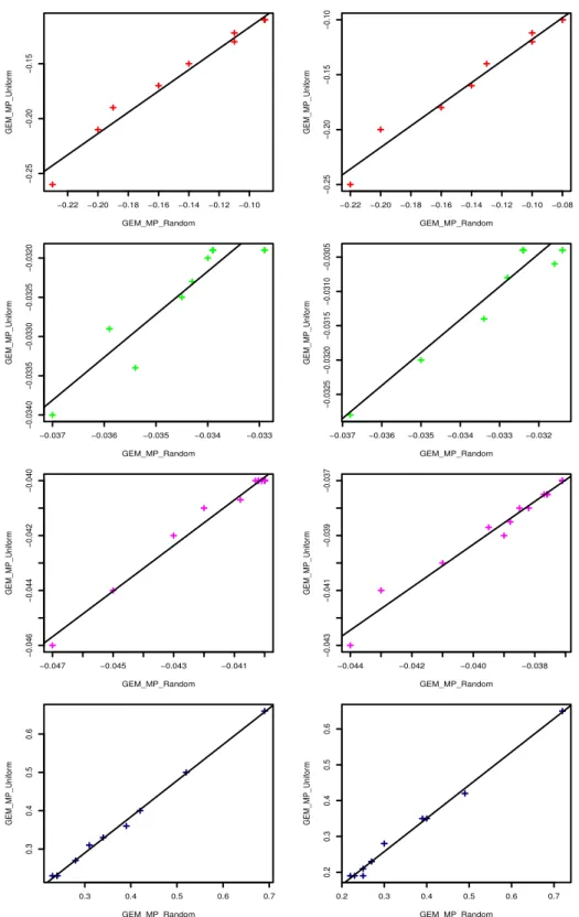
vs. the average CLL of GEM-MP-Uniform (y-axis) for Cora (red), Yeast (green) and UW-CSE (magenta) at two determinism zones, re-spectively. Bottom: the average KL-divergence of GEM-MP-random vs. the average KL-divergence of GEM-MP-Uniform for 20 × 20 grids of Ising model at determinism zone1 [0% − 20%] (left-blue) and at de-terminism zone2 [20% − 40%] (blue) during iterations. . . . 92 Figure 5.1 a) Propositional-BP. b) From left to right, the steps of PR-BP inference
algorithm. . . 100 Figure 5.2 Inference time (secs) vs. number of objects in Yeast at 25% amount of
determinism. . . 104 Figure 5.3 Inference time (secs) vs. number of objects in Yeast at 37.5% amount
of determinism. . . 105 Figure 5.4 Inference time (secs) vs. number of objects in UW-CSE at 9.7% amount
of determinism. . . 106 Figure 5.5 Inference time (secs) vs. number of objects in UW-CSE at 38.9%
amount of determinism. . . 107 Figure 5.6 Inference time (secs) vs. number of objects in Cora at 12.5% amount
of determinism. . . 108 Figure 5.7 Inference time (secs) vs. number of objects in Cora at 25% amount of
determinism. . . 109 Figure 5.8 Inference memory space (bytes) vs. number of objects in Cora at 25%
amount of determinism. . . 110 Figure 5.9 Inference memory space (bytes) vs. number of objects in UW-CSE at
25% amount of determinism. . . 111 Figure 6.1 (Left) An example factor graph G that involves grounding clauses F =
{fa, fb, fc, fd}, and three ground atoms {X1, X2, X3}, where dashed and
solid lines represent “-” and “+” appearance of the atoms, respectively. (Right) The extended factor graph ˆG, after adding auxiliary mega-node vari-ables P = {P1, P2, P3} and auxiliary factor nodes Φ = {ϕ1, ϕ2, ϕ3}, which
yields a set of extended factors ˆF =nfˆa, ˆfb, ˆfc, ˆfd o
. . . 114 Figure 6.2 Cost vs. Time: average cost of unsatisfied clauses (smaller is better)
Figure 6.3 Cost vs. Time: average cost of unsatisfied clauses (smaller is better) against time for Cora at 250 objects. . . 134 Figure 6.4 Cost vs. Time: average cost of unsatisfied clauses (smaller is better)
against time for Cora at 1000 objects. . . 135 Figure 6.5 Cost vs. Time: average cost of unsatisfied clauses (smaller is better)
against time for WebKB at 50 objects. . . 136 Figure 6.6 Cost vs. Time: average cost of unsatisfied clauses (smaller is better)
against time for WebKB at 250 objects. . . 137 Figure 6.7 Cost vs. Time: average cost of unsatisfied clauses (smaller is better)
against time for WebKB at 1000 objects. . . 138 Figure 6.8 Cost vs. Time: average cost of unsatisfied clauses (smaller is better)
against time for Yeast at 50 objects. . . 139 Figure 6.9 Cost vs. Time: average cost of unsatisfied clauses (smaller is better)
against time for Yeast at 250 objects. . . 140 Figure 6.10 Cost vs. Time: average cost of unsatisfied clauses (smaller is better)
against time for Yeast at 1000 objects. . . 141 Figure 6.11 Cost vs. cooling parameter: average cost of unsatisfied clauses (smaller
is better) against different values of cooling parameter y of WSP-Dec algorithm for Cora. . . 142 Figure 6.12 Cost vs. cooling parameter: average cost of unsatisfied clauses (smaller
is better) against different values of cooling parameter y of WSP-Dec algorithm for WebKB. . . 143 Figure 6.13 Cost vs. cooling parameter: average cost of unsatisfied clauses (smaller is
better) against different values of cooling parameter y of WSP-Dec algorithm for Yeast. . . 144
LIST OF SYMBOLS AND ABBREVIATIONS
BP Belief Propagation
CCC Double loop (Concave-Convex) Procedure CLL average Conditional Log marginal-Likelihood CS Constraint Satisfaction
GAC Generalized arc Consistency
GEM-MP Generalized arc consistency Expectation Maximization Message Pass-ing
Gibbs MCMC (Gibbs Sampling)
KL The average Kullback-Leibler divergence LBP Loopy Belief Propagation
L-IM Lifted MCMC (Importance Sampling)
L2-Convex Sequential Message Passing on the Convex-L2 Bethe Free Energy MAP Maximum-A-Posteriori Inference
MAR Marginal Inference
MAX-SAT Maximum Satisfiablility Problem MRF Markov Random Field
MF Mean Field Approximation MLN Markov Logic Network
ML Machine Learning
pAc Probabilistic Arc-Consistency PR Preference Relaxation
PGAC Probabilistic Generalized Arc-Consistency PGM Probabilistic Graphical Model
PG Propositional Grounding
SAT Propositional Satisfiability Problem SP Survey Propagation
SRL Statistical Relational Learning RBP Residual Belief Propagation
VEM Variational Expectation Maximization
WSP-χ Family of Weighted Survey Propagation Algorithms WSP-Dec WSP-χ Inspired Decimation
LIST OF APPENDICES
CHAPTER 1 INTRODUCTION
We provide here an overview of our research and the motivation behind it. Next, we explain our research problems and formalize our objectives through some concise research questions. We then summarize our contributions and conclude with an outline of this thesis.
1.1 Overview and Motivations
Graphical models that involve cycles and determinism are applicable to a growing number of applications in different research communities, including machine learning, statistical physics, constraint programming, information theory, bioinformatics, and other sub-disciplines of ar-tificial intelligence. Accurate and scalable inference within such graphical models is thus an important challenge that impacts a wide number of communities. Inspired by the sub-stantial impact of statistical relational learning (SRL) (Getoor and Taskar, 2007), Markov logic (Richardson and Domingos, 2006) is a powerful formalism for graphical models that has made significant progress towards the goal of combining the powers of both first-order logic and probability. This allows one to address relational and uncertain dependencies in data. However, for the second part of the goal, and in practice, inference always tends to give poor results in the presence of both cycles and determinism and can be problematic for learning when using it as a subroutine.
Furthermore, commonly in SRL models it has been convenient to convert formulas to conjunc-tive normal form (CNF) and to propositionalize the theory to a grounded network of clauses wherein any probabilistic inference can be applied for reasoning about uncertain queries. In such cases, the logical structure within the network can be problematic for certain inference procedures and often represents a major bottleneck when faced with instances close to the satisfiability threshold. This situation in fact frequently occurs in SRL instances of real-world applications. In addition, this approach can be very time consuming: the grounded network is typically large, which slows down inference, and this also can be problematic, especially for the scalability of inference.
1.2 Problem Statement and Limitations
Our dissertations here revolve around improving the accuracy and scalability of inference for three problems related to computing marginal probabilities (marginals for short) and MAP assignments on graphical models that involve cycles and determinism within an underlying
probabilistic network of a size such that inference in the network poses problems for all known methods.
1.2.1 Problem 1
To compute marginals, loopy belief propagation (LBP) is a commonly used message-passing algorithm for performing approximate inference in graphical models in general, including models instantiated by an underlying Markov Logic. However, LBP often exhibits erratic behavior in practice. In particular, it is still not well understood when LBP will provide good approximations in the presence of cycles and when models possess both probabilistic and deterministic dependencies. Therefore, the development of more accurate and stable message passing based inference methods is of great theoretical and practical interest. Per-haps surprisingly, belief propagation achieves good results for coding theory problems with loopy graphs (Mceliece et al., 1998; Frey and MacKay, 1998). In other applications, how-ever, LBP often leads to convergence problems. In general LBP therefore has the following limitation:
Limitation 1. In the presence of cycles, LBP is not guaranteed to converge.
From a variational perspective, it is known that if a factor graph has more than one cycle, then the convexity of the Bethe free energy is violated. It is known that the local optima of the Bethe free energy correspond to fixed points of LBP, and it has been proven that violating the uniqueness condition for the Bethe free energy generates several fixed points in the space of LBP’s marginal distributions (Heskes, 2004; Yedidia et al., 2005). A graph involving a single cycle has a unique fixed point and usually guarantees the convergence of LBP (Heskes, 2004). From the viewpoint of local search, LBP performs a gradient-descent/ascent search over the marginal space, endeavoring to converge to a fixed point (i.e., local optimum, see Heskes, 2002). Heskes viewpoint is that the problem of non-convergence is related to the fact that LBP updates the unnormalized marginal of each variable by computing a coarse geometric average of the incoming messages received from its neighboring factors (Heskes, 2002). Under Heskes’ line of analysis, LBP can make large moves in the space of the marginals and therefore it becomes more likely to overshoot the nearest local optimum. This produces an orbiting effect and increases the possibility of non-convergence. Other lines of analysis are based on the fact that messages in LBP may circulate around the cycles, which can lead to local evidence being counted multiple times (Pearl, 1988). This, in turn, can aggravate the possibility of non-convergence. In practice, non-convergence occasionally appears as oscillatory behavior when updating the marginals (Koller and Friedman, 2009). The solid black curves in Figure 1.1 are empirical examples that depict the non-convergence of LBP
due to cycles.
Figure 1.1 A preliminary experiment illustrates the effects of cycles and determinism on the convergence behaviour of LBP in Cora dataset (Singla and Domingos, 2006a) (left) and Yeast dataset (Singla and Domingos, 2006a) (right). These datasets and their models are publicly available at the alchemy website: http://alchemy.cs.washington.edu/data/
Determinism also plays a substantial role in reducing the effectiveness of LBP (Heskes, 2004). It has been observed empirically that carrying out LBP on cyclic graphical models with determinism is more likely to result in a two-fold problem of non-convergence or incorrectness of the results (Mooij and Kappen, 2005; Koller and Friedman, 2009; Potetz, 2007; Yedidia et al., 2005; Roosta et al., 2008). A second limitation of LBP could thus be formulated as: Limitation 2. In the presence of determinism (a.k.a. hard clauses), LBP may deteriorate to inaccurate results.
In its basic form LBP also does not leverage the local structures of factors, handling them as black boxes. Using Markov logic as a concrete example, LBP often does not take into consideration the logical structures of the underlying clauses that define factors (Gogate and Domingos, 2011). Thus, if some of these clauses are deterministic (e.g., hard clauses) or have extreme skewed probabilities, then LBP will be unable to reconcile the clauses. This, in turn, impedes the smoothing out of differences between the messages. The problem is particularly acute for those messages that pass through hard clauses which fall inside dense cycles. This can drastically elevate oscillations, making it difficult to converge to accurate results, and leading to the instability of the algorithm with respect to finding a fixed point (see pages 413-429 of Koller and Friedman, 2009, for more details). The solid red curves in Figure 1.1 illustrate empirically the increase in the non-convergence of LBP due to cycles and determinism. On the flip side of this issue Koller and Friedman point out that one can
prove that if the factors in a graph are less extreme — such that the skew of the network is sufficiently bounded — it can give rise to a contraction property that guarantees convergence (Koller and Friedman, 2009).
Although LBP has been scrutinized both theoretically and practically in various ways, most of the existing research either avoids the limitation of determinism when handling cycles, or does not take into consideration the limitation of cycles when handling determinism.
1.2.2 Problem 2
It is common for many real-world problems to have expressive graphical models that combine deterministic and probabilistic dependencies. In the world of SRL, the former often appear in the form of mandatory (i.e. hard) constraints that must be satisfied in any world with a non-zero probability. The latter are typically formulated as preferences (i.e. soft constraints), and dissatisfying them is not impossible, but less probable. Thus, if a query atom X which is involved with a set of constraints C = {H, S} (where H and S are its subsets of hard and soft constraints respectively) violates one of the hard constraints h in H, then its marginal probability will be zero, even if it satisfies its other hard and soft constraints in C − {h}. A variable violates a hard constraint if there is a truth value for that variable such that the constraint is violated in all possible worlds consistent with that truth value assignment to the variable and the evidence. Current inference approaches do not exploit the fact that there is no need to consider irrelevant computations (and memory usage) with soft constraints S, since using only hard constraints H should be sufficient to compute that its marginal probability P (X) is zero.
Limitation 3. In relational domains, where we have millions of query atoms each involved with thousands of constraints, such irrelevant computations greatly weaken the scalability of the inference, especially if most query atoms have a tendency to violate hard constraints. Inspired by the sparseness property of relational domains, the marginal probability of the vast majority of query atoms being true is frequently zero. Potentially this is due to the violation of hard constraints that have at least one false precondition query atom.
1.2.3 Problem 3
To compute MAP assignments, it has been proven that maximum-a-posteriori (MAP) infer-ence is equivalent to solving a weighted MAX-SAT problem (i.e., where one finds the most
probable truth assignment or “MAP” solution that maximizes the total weight of satisfied clauses) (Park, 2002). A simple approach to tackle MAP inference is to use off-the-shelf local search algorithms that are designed to efficiently solve weighted MAX-SAT instances. For example MaxWalkSAT (Kautz et al., 1997; Selman et al., 1993) was recently applied as a conventional MAP inference method in probabilistic graphical models (Richardson and Domingos, 2006). However, it is known that for real world applications, and in relational domains, models are normally translated into grounded networks featuring high densities.1
From the point of view of satisfiability, if the density of the grounded network is close to a satisfiability threshold, then the (MAP) assignments in the solution space are clustered (Mann and Hartmann, 2010). This clustering means that the (MAP) assignments belonging to the same cluster are close to each other (e.g., in terms of Hamming distance). It has been shown that such clustering in the solution space exists not only for uniform random satisfi-ability, but also for some structured satisfiability instances that follow realistic and natural distributions (Hartmann and Weigt, 2006; Zhang, 2004; Gomes et al., 2002; Parkes, 1997), similar to real-world problems that are modeled as MLNs (e.g., social networks, as shown by Kambhampati and Liu (2013)). In general, using local search algorithms for MAP inference frequently has the following limitations due to the clustering of the solution space:
Limitation 4. Usually, the existence of many clusters is an indication of a rugged en-ergy landscape, which then also gives rise to many local optima. This often hinders the performance of most local search algorithms because they can get stuck in a local optimum (Montanari et al., 2004).
Limitation 5. Another possible consequence of the clustering of the solution space is that the search space fractures dramatically with a proliferation of ‘metastable’ clusters (Chavas et al., 2005). This acts as a dynamic trap for local search algorithms, including MaxWalkSAT, since they can get stuck in one such ‘metastable’ cluster at a local optimum (Kilby et al., 2005; Chavas et al., 2005). On the flip side of the issue, if the clauses capture complex structures (e.g., relational dependencies) then the clusters tend to decompose into an exponentially small fraction of (MAP) assignments (Mann and Hartmann, 2010). So there is not even any guarantee of getting into a cluster that contains an optimal solution. Clearly, this all greatly weakens the possibility that a local search can converge to an optimal solution, particularly for SRL applications (Riedel, 2008).
It is well known that techniques such as marginalization-decimation based on the max-product BP algorithm (Wainwright et al., 2004; Weiss and Freeman, 2001), can be used to help local search find an optimal MAP solution, but it is also believed that BP does not
converge due to strong attraction in many directions (Kroc et al., 2009; Khosla et al., 2009). That is, max-product BP fails because its local computations may obtain locally optimal as-signments corresponding to different clusters, but these cannot be combined to find a global MAP solution (Kroc et al., 2009).
Fortunately, it is likely that in each cluster there is a certain fraction of ‘frozen’ ground atoms (Achlioptas and Ricci-Tersenghi, 2009) that are fixed in all (MAP) solutions within the cluster, while the others can be varied subject to some ground clauses. These frozen ground atoms are known as ‘cluster backbones’ (Kroc et al., 2008). Thus, one relatively crude but useful way to obtain a portion of a solution in the cluster is by finding the cluster backbones.
1.3 Research Questions and Objectives
We formalize our objectives through some concise research questions as follows:
• To address Limitations 1 and 2 of LBP discussed above, our first objective is to answer the following research questions:
– (RQ1) Does updating the marginals such that we do not overshoot the nearest fixed point diminish the threat of non-convergence of LBP?
– (RQ2) Are constraint satisfaction techniques able to help address the challenges resulting from determinism in the graphical models?
• To address Limitation 3, and avoid irrelevant computations involving preferences when performing inference, our second objective is to answer the following research question: – (RQ3) Can relaxing soft constraints or preferences be helpful to avoid irrelevant computations involving preferences? That is to say, can performing the inference by using only hard constraints (determinism) be exploited to reduce problem size? • To address Limitations 4 and 5 of local search algorithms, which are due to search
space clustering, our third objective is to answer the following research questions: – (RQ4) Can we derive a method to identify backbones in a cluster involving
po-tentially optimal MAP solutions?
– (RQ5) Can the cluster backbones be used to scale MAP inference?
1.4 Summary of the Contributions
Through the research presented in this thesis, we achieve our objectives by answering the research questions above. This has led to our main contributions summarized as follows:
• Generalized arc-consistency Expectation-Maximization Message-Passing (GEM-MP), a novel message-passing algorithm for applying variational ap-proximate inference to graphical models.
In GEM-MP, we first re-parameterized the factor graph in such a way that the infer-ence task (that could be performed by LBP inferinfer-ence on the original factor graph) is equivalent to a variational EM procedure. Then, we take advantage of the fact that LBP and variational EM can be viewed in terms of different types of free energy mini-mization equations. We formulate our Message-Passing structure as the E and M steps of a variational EM procedure (Beal and Ghahramani, 2003; Neal and Hinton, 1999). This variational formulation leads to the synthesis of new rules that update marginals by maximizing a lower bound of the model evidence such that we never overshoot the model evidence (Answering research question RQ1 ). In addition, in the corresponding Expectation step of GEM-MP, the constructed expected log marginal-likelihood has been defined according to the posterior distribution over local entries of the logical clauses that define factors. This enables us to exploit their logical structures by ap-plying a generalized arc-consistency concept (Rossi et al., 2006), and to use that to perform a variational mean-field approximation when updating the marginals. This significantly amends smoothing out the marginals to converge correctly to a stable con-vergent fixed point in the presence of determinism (Answering research question RQ2 ). Our experiments on real-world problems demonstrate the increased accuracy and con-vergence of GEM-MP compared to existing state-of-the-art inference algorithms such as MC-SAT, LBP, and Gibbs sampling, and convergent message passing algorithms such as the Concave-Convex Procedure (CCCP), Residual BP, and the L2-Convex method. • Preference Relaxation (PR), a new two-stage strategy that uses the deter-minism (i.e., hard constraints) present in the underlying model to improve the scalability of relational inference.
The basic idea of PR is to diminish irrelevant computational time and memory, which are due to preference constraints. To do so, in a first stage PR starts by relaxing preferences and performing inference with hard constraints only in order to obtain the zero marginals for the query ground atoms that violate the hard constraints. It then filters these query atoms (i.e., it removes them from the query set) and uses them to
enlarge the evidence database. Then in a second stage preferences are reinstated and inference is performed on a grounded network that is constructed based on both a filtered query set and an expanded evidence database obtained in the first stage. PR substantially reduces the effective size of the constructed grounded network, potentially with a loss of accuracy. (Answering research question RQ3 ). Experiments on real-world applications show how this strategy substantially scales inference with a minor impact on accuracy.
• Weighted Survey Propagation-inspired Decimation (WSP-Dec), a novel fam-ily of message passing algorithms for applying MAP inference to graphical models.
In WSP-Dec, we first describe a novel family of extended factor graphs, specified by the parameter χ ∈ [0, 1]. These factor graphs are re-parameterized in such a way that they define positive joint probabilities over max-cores. These max-cores are natural interpretations of core assignments (Maneva et al., 2007) that satisfy a set of clauses with maximal weights. We then show that applying BP message-passing to this family recovers a family of Weighted SP algorithms (WSP-χ), ranging from pure Weighted SP (WSP-1) to standard max-product BP (WSP-0). The magnetization of the marginals computed by any WSP-χ algorithm can be used to obtain backbones (i.e., frozen ground atoms) of a cluster involving potentially optimal MAP solutions (Answering research question RQ4 ). The cluster backbones are not only a portion of the optimal solutions in the cluster, but they can also be used to enlarge the evidence database and shrink the query set. Therefore, iteratively fixing them results in a reduction of the complex parts of the grounded network, which afterwards can be simplified to a scalable one that is then solved accurately using any conventional MAP method (Answering research question RQ5 ). Hence, integrating WSP-χ as pre-processing with a MaxWalkSAT al-gorithm in a decimation procedure produces a family of Weighted Survey Propagation-inspired decimation (WSP-Dec) algorithms for applying MAP inference to SRL models (Answering research question RQ6 ). Our experiments on real-world applications show the promise of WSP-χ to improve the accuracy and scalability of MAP inference when integrated with local search algorithms such as MaxWalkSAT.
• Lazy-WSP-χ, a novel lazy variant of weighted Survey Propagation for effi-cient relational MAP inference.
In Lazy-WSP-χ, we start by grounding the network lazily, and maintaining only active ground clauses and their active ground atoms that are sufficient to answer the queries. We then call WSP-χ to scale the lazy ground network, which was built using those
active clauses and atoms, by fixing the frozen active atoms. Thus, Lazy-WSP-χ mainly differs from WSP-χ in both the initial set of underlying query atoms and clauses. Our experiments on real-world applications show how using the lazy variants of WSP-χ greatly improves the scalability of MAP inference.
• Lazy-based inference, a hybrid inference approach that combines PR-based inference with lazy inference to greatly improve the scalability of marginal inference.
One key advantage of our proposed PR strategy is that it can be combined with other state-of-the-art approaches which improve the scalability of inference, such as Lazy and Lifted. In Lazy-PR-based inference, we start by maintaining only the active-awake hard constraints and their atoms. We then call the relational inference on the ground network, which was built using those maintained clauses and atoms. After reaching a fixed point, we filter active-awake query atoms and enlarge the evidence database. The experimental evaluations on real-world applications show that hybridizing Lazy-PR-based inference with relational inference algorithms improves their efficiency for computing marginals.
Through our experimental evaluations in this thesis, we have focused on Markov logic and Ising models, but it is worth noting that all the main proposed techniques (GEM-MP, PR and WSP-χ) and their lazy variants are applicable to other representations of SRL models, including standard graphical models defined in terms of factor graphs.
1.5 Organization of the Dissertation
The remainder of this thesis is organized as follows.
Part I is about the state of the art, and it consists of two chapters:
• Chapter 2 presents the necessary background of the techniques and methods useful to understand this thesis.
• Chapter 3 presents a thorough discussion for the related work relevant to this thesis. Part II consists of three chapters in which we present our contributions:
• Chapter 4 demonstrates our Generalized arc-consistency Expectation-Maximization Message-Passing (GEM-MP) for applying variational approximate inference to graph-ical models in the presence of cycles and determinism. The contents of this chapter are largely extracted from our paper:
Mohamed-Hamza Ibrahim, Christopher Pal and Gilles Pesant. “Improving Message-Passing Inference in the Presence of Determinism and Cycles”. Currently under review in the Machine Learning Journal (MLJ).
• Chapter 5 explains our Preference Relaxation (PR) strategy that uses the determin-ism present in the underlying model to improve the scalability of relational inference. It also demonstrates how to combine PR-based inference with lazy inference. The contents of this chapter are based on our paper:
Mohamed-Hamza Ibrahim, Christopher Pal and Gilles Pesant. “Exploiting determinism to scale relational inference”. Published in Proceedings of the Twenty-Ninth National Conference on Artificial Intelligence (AAAI’15) in 2015 (Ibrahim et al., 2015).
• Chapter 6 demonstrates our Weighted Survey Propagation-inspired Decimation (WSP-Dec), a family of algorithms to handle MAP inference in the presence of clustered search space. It also explains lazy variants of this family of algorithms. The contents of this chapter are largely extracted from our paper:
Mohamed-Hamza Ibrahim, Christopher Pal and Gilles Pesant. “Exploiting Cluster Backbones to Improve MAP Inference in Relational Domains”. Submitted to Journal of Artificial Intelligence Research (JAIR).
Chapter 7 concludes the thesis by revisiting our major contributions and sketching our possible opportunities for future research directions.
CHAPTER 2 BACKGROUND
To set the stage for this thesis, in this chapter we review basic concepts and methods that are necessary to understand our research by using an explanatory example, presented in Table 2.1. This example is an excerpt of the knowledge base for the Cora dataset (Singla and Domingos, 2006a). Suppose that we are given a citation database in which each citation has author, title, and venue fields. We wish to know which pairs of citations refer to the same citation and the same authors (i.e., both the SameBib and SameAuthor relations are unknown). For simplicity, suppose that our goal will be to predict the SameBib ground atoms’ marginals and compute their most probable truth assignment (i.e., MAP solution). The first part of the goal refers to the marginal inference problem and the second refers to the maximum-a-posteriori (MAP) inference problem. At this point, let us first express our prerequisite basic definitions.
Table 2.1 An excerpt of the knowledge base for the Cora dataset. The atoms SameBib and SameAuthor are unknown. Ar() is an abbreviation for atom Author(), SAr() for SameAu-thor(), and SBib() for SameBib(). a1, a2 represent authors and r1, r2, r3 represent citations.
Rule First-order Logic Weight
Regularity ∀a1, a2, ∀r1, r2, Ar(r1, a1)∧Ar(r2, a2)∧SAr(a1, a2) ⇒ SBib(r1, r2) 1.1
Transitivity ∀r1, r2, r3, SBib(r1, r2) ∧ SBib(r2, r3) ⇒ SBib(r1, r3) ∞
Clausal Form
Regularity ¬Ar(r1, a1) ∨ ¬Ar(r2, a2) ∨ ¬SAr(a1, a2) ∨ SBib(r1, r2) 1.1
Transitivity ¬SBib(r1, r2) ∨ ¬SBib(r2, r3) ∨ SBib(r1, r3) ∞
2.1 Basic Notation and Definitions
A first-order knowledge base (KB) is a set of formulas in first-order logic (FOL).
Definition 1 (First-Order Logic (FOL)). The set of terms of FOL (also known as first-order predicate calculus) is defined by the following rules:
• A variable is a term
• If P is a predicate symbol with t1, . . . , tn terms and n ≥ 0, then P (t1, . . . , tn) is an
atomic statement.
In FOL, each formula is a sentential formula (e.g., ∀X ∃Z f (X, Z)), where ∀ is the universal quantifier, and ∃ is the existential quantifier. f (X, Z) is the scope of the respective quantifier, and any occurrence of variable X or Z in the scope of a quantifier is bound by the closest ∀X or ∃Z.
The set of sentential formulas of first-order predicate calculus is defined by the following rules:
• Any atomic statement is a sentential formula
• If f1 and f2 are sentential formulas, then ¬f1, f1∧ f2, f1∨ f2, and f1 ⇒ f2 (f1 implies
f2) are sentential formulas.
In formulas of first-order predicate calculus, all variables are object variables serving as ar-guments of functions and predicates.
Definition 2 (Conjunctive Normal Form (CNF)). A formula is in conjunctive normal form (or clausal normal form) if it is represented as a conjunction of clauses, where a clause is a disjunction of literals- a literal represents either a variable or its negation.
For the purpose of probabilistic (and automated) inference, it is often convenient to convert FOL formulas to a clausal form (CNF).1 For instance, as shown in Table 2.1, we convert
FOL formulas of the explanatory example into a clausal form (CNF).2 This is known as
propositional grounding.
Definition 3 (Propositional grounding (PG)). PG is the process of replacing a first-order Knowledge Base (KB) by an equivalent propositional one (Richardson and Domingos, 2006). In finite domains, inference over a first-order KB can be performed by propositional grounding followed by satisfiability testing. But in order to apply a satisfiability solver we need to create a Boolean variable for every possible grounding of every predicate in the domain and a propositional clause for every grounding of every first-order clause.
1This includes the removal of the existential quantiers by Skolemization, which is not sound in general.
However, in finite domains an existentially quantied formula can simply be replaced by a disjunction of its groundings.
2Note that the weights that are associated with the FOL formulas in Table 2.1 will be used later to extend
the FOL formulation with Markov Logic– one of the most powerful graphical model representations – as will be discussed in Section 2.2.2
After propositional grounding, we get a formula F , which is a conjunction of m ground clauses. We use fi ∈ F to denote a ground clause which is a disjunction of literals built
from X , where X = {X1, X2, . . . , Xn} is a set of n Boolean random variables representing
ground atoms. Each fi is associated with the pair ( ˆwi, Xfi), where ˆwi is its weight and the set Xfi ⊆ X corresponds to the variables appearing in its scope. Both “+” and “−” will be used to denote the positive (true) and negative (false) appearance of the ground atoms. A joker “∗” will be used to denote the “don’t care” state of a variable Xj. That is, the
assignment Xj = ∗ means that the variable Xj is free to take either “+” or “−” since the
clauses containing it should be already satisfied by other variables, and the value of Xj does
not matter. We use Yi as a subset of satisfying (or valid) entries of ground clause fi, and
yk ∈ Yi, k ∈ {1, .., |Yi|} denotes each valid entry in Yi, where the local entry of a factor
is valid if it has non-zero probability. We use fs
i (resp. fih) to indicate that the clause fi
is soft (resp. hard); the soft and the hard clauses are included in the two sets Fs and Fh
respectively. The sets FXj+ and FXj− include the clauses that contain positive and negative literals for ground atom Xj, respectively. Thus FXj = FXj+∪ FXj− denotes the whole of Xj’s clauses, and its cardinality as
FXj
. For each ground atom Xj, we use βXj =
h
βX+j, βX−ji to denote its positive and negative marginal probabilities, respectively. BX denotes the whole
set of X ’s marginals.
Definition 4. For a ground clause fi, we define si,j (resp. ui,j) as the value of a ground
atom Xj ∈ {1, 0} that satisfies (resp. violates) fi. Therefore, fi is satisfied if and only if at
least one of its ground atoms Xj is equal to si,j.
Xs
fi and X
u
fi are used to denote the two disjoint subsets of the ground atoms that are satisfying and violating fi, respectively. Now from the above definition, we have the following sets:
FXj+ = {fi ∈ FXj; si,j = 1}, FXj− = {fi ∈ FXj−; si,j = 0} (2.1a) Fs(j) = {f i ∈ FXj; Xj = si,j}, F u(j) = {f i ∈ FXj; Xj = ui,j} (2.1b) Ffsi(j) = {fk∈ FXj \ {fi}; si,j = sk,j}, F u fi(j) = {fk∈ FXj\ {fi}; si,j 6= sk,j} (2.1c) where we use Fs(j), Fu(j) to denote the two disjoint subsets of the ground clauses that are
satisfied and violated by Xj, respectively. We use Ffsi(j) (resp. F
u
fi(j)) to denote the subset of ground clauses that agree (resp. disagree) with fi about Xj.
Definition 5. (Maneva et al., 2007) We say that a variable Xj is the unique satisfying
variable for a clause fi ∈ F if it is assigned si,j whereas all other variables in the clause
variable for fi. That is to say, it satisfies an indicator function as follows:
CONi,j(Xfi) = Ind(Xj is the unique variable satisfying fi) (2.2) Where Ind(Predicate) returns 1 if the Predicate is true and 0 otherwise. The variable Xj is
said to be unconstrained if it has 0 or 1 value and it violates CONi,j(Xfj) for each clause fi ∈ FXj that involves it, or it has a joker ∗ value.
Definition 6. (Chieu and Lee, 2009) A complete assignment X:
• Satisfies a clause fi if and only if (i) fi contains a constrained variable Xj that is set
to si,j, or (ii) fi contains at least two unconstrained joker variables.
• Violates a clause fi if and only if all its variables Xj ∈ Xfi are set to ua,i.
• Is invalid for a clause fi if and only if exactly one variable Xj takes a joker value ∗
and all its other variables Xk ∈ Xfi\ Xj are set to ui,k.
The complete assignment X is valid for a F if it is valid for all of its clauses. Note that the above definition of the invalid complete assignment reflects the interpretation that the joker value “∗” is a “don’t care” state for variable Xj: clauses involving a variable Xj = ∗
should be already satisfied by other variables, and the value of Xj does not matter. This
in fact means that Xj = ∗ cannot be the last remaining possibility of satisfying any clause.
So, if the other variables violate the clause and the remaining variable Xj is a joker, then
the complete assignment is neither satisfying nor violating the clause because in this case we have two possibilities for Xj = ∗: one makes the complete assignment satisfying and the
other makes it violating. Thus we say that the complete assignment is invalid. In the case where a clause contains two variables set to joker, the clause can be satisfied by either one of these two variables, so the other variable can take the “don’t care” value.
2.2 Probabilistic Graphical Models
Now after expressing the basic notation and definitions, let us recall our goal of solving the marginal and MAP inference problems in the explanatory example. The first step, before carrying out the inference, is to represent the problem as a probabilistic graphical model (PGM). PGM is a graphical model that efficiently defines and describes a probabilistic model (e.g., joint distribution of the variables). PGMs are often classified into two major classes: Bayesian networks (BNs) and Markov random fields (MRFs).
Markov random fields (MRFs), also known as undirected graphical models, compactly rep-resent a joint distribution over X as a product of potentials defined on subsets of variables (see Koller and Friedman, 2009). In order to motivate the use of MRFs, below we describe briefly two MRFs’ models that will be used frequently throughout the thesis:
• Ising Models (Ising)
• Markov Logic Networks (MLNs)
2.2.1 Ising Models
The Ising model is an example of an MRF that arose from statistical physics. It was originally used for modeling the behavior of magnets. In particular, let Xi ∈ {1, 0} represents the spin
of an atom, which can either be spin down (i.e., 0 ↓) or up (i.e., 1 ↑). In some magnets, called ferro-magnets, neighboring spins tend to line up in the same direction, whereas in other kinds of magnets, called anti-ferromagnets, the spins want to be different from their neighbors. We can model this as an MRF by creating a graph in the form of a 2D or 3D lattice, and connect neighboring variables, as in Figure 2.1, by using a set of pairwise clique potentials:
φij(Xi, Xj) = eθij if X i = Xj e−θij Otherwise (2.3)
Figure 2.1 A 2D lattice represented as undirected graphical model. The red node X8 is
independent of the other black nodes given its neighbors (blue nodes)
The 2D Ising models with arbitrary topology are a specific subset of the canonical (pairwise) MRFs. Assume that X = {X1, . . . , Xn} is a set of binary random variables (representing
the spins) that are Bernoulli distributed. In a 2D Ising model I = ((X , E ); θ) we have an undirected graph consisting of the set of all variables X , a set of edges between variables E , and a set of parameters θ = {θi, θij}. The model can be given as
p(X = x) = Zθ−1 energy function z }| { e h P (Xi,Xj )∈Eθij·XiXj+ P Xi∈Xθi·Xi i (2.4a) = Zθ−1 " Y (Xi,Xj)∈E φij(Xi,Xj) z }| { eθij·1(Xi,Xj ) # × " Y Xi∈X φi(Xi) z }| { eθi·Xi # (2.4b)
where Zθ is the normalizing constant. 1(Xi,Xj) is an indicator function that equals one when Xi = Xj. Otherwise it is equal to zero. Both {θi} and {θij} are the parameters of
uni-variate potentials {φi(Xi)} and pairwise potentials {φij(Xi, Xj)}, respectively. Typically,
the parameters {θi} are drawn uniformly from U [−df, df], where df ∈ R. For pairwise
potentials, the parameters {θij} are chosen as η · C where we sample η in the range [−df, df]
having some nodes to agree and disagree with each other. C is also a chosen constant. Higher values of C impose stronger constraints, leading to a harder inference task.
2.2.2 Markov Logic Networks
A Markov Logic Network (MLN) (Richardson and Domingos, 2006) is a set of first-order logic formulas (or CNF clauses), each of which is associated with a numerical weight w. Larger weights w reflect stronger dependencies, and thereby deterministic dependencies have the largest weight (w → ∞), in the sense that they must be satisfied. We say that a clause has deterministic dependency if at least one of its entries has zero probability. With finite sets of constants that are domains to atoms, we can build a Markov logic network that has the following:
• One binary node for each possible grounding of each atom appearing in each clause. The value of the node is 1 if the ground atom is true, and 0 otherwise.
• One feature for each possible ground clause fi. The value of this feature is 1 if the
ground formula is true, and 0 otherwise. The weight of the feature is the weight wi
associated with fi, where the weight attached to each ground clause reflects its strength
dependency.
The power of MLNs appears in their ability to bridge the gap between logic and probability theory. Thus it has become one of the preferred probabilistic graphical models for
repre-senting both probabilistic and deterministic knowledge, with deterministic dependencies (for short we say determinism) represented as hard clauses, and probabilistic ones represented as soft clauses.
To understand the semantics of Markov logic, recall the explanatory example in Table 2.1. In this example, Markov logic enables us to model the KB by using rules such as the following: (1) Regularity rules of the type that say “if the authors are the same, then their records are the same.” This rule is helpful but innately uncertain (i.e., it is not true in all cases). Markov logic considers this rule as soft and attaches it to a weight (say, 1.1); and (2) Transitivity rules that state “If one citation is identical to two other citations, then these two other citations are identical too.” These types of rules are important for handling non-unique names of citations. Therefore, we suppose that Markov logic considers these rules as hard and assigns them an infinite weight.3
2.2.3 Factor Graphs
For the purpose of solving inference problems, it is often convenient to convert MRFs into a different representation called factor graph.
Definition 7 (Factor Graphs (FG)). A factor graph is a bipartite graph involving two types of nodes: variables and factors (i.e., constraints or clauses). Associated with each such node is a variable or a factor over variables, respectively. Typically, we will denote a factor graph G = (X ; F ) in terms of its variables X and factors F .
Note that FG introduce additional nodes for representing the potentials of MRFs. This allows the model to be more explicit about the factorization when defining its joint distribution, which can be written as a product of factors as follows:
P (X1, · · · , Xn) = 1 Z Y fi∈F fi(Xfi) (2.5)
Where Z is a normalization constant that enforces the factorization to represent a probability distribution that sums to one. Factor graphs unify directed and undirected graphs with the same representation. Thus they can be used to represent undirected graphs such as MRFs, where the factors will be the potential functions. If the factor graphs are being used to represent directed graphs like BNs, then the factors will be the local conditional distributions of each node, and here the extra normalization term in the joint distribution is not needed.
Figure 2.2 Grounded factor graph obtained by applying clauses in Table 2.1 to the constants: {Gilles(G), Chris(C)} for a1and a2; {C1, C2} for r1, r2, and r3. The factor graph involves: 12
ground atoms in which 4 are evidence (dark ovals) and 8 are non-evidence (non-dark ovals); 24 ground clauses wherein 8 are hard (Fh = {f1, · · · , f8}) and 16 are soft (Fs = {f9, · · · , f24}).
For instance, the Ising models in Eq. (2.4b) can be represented as factor graphs, where vari-ables Xi ∈ X are represented as variable nodes and potentials {φi(Xi)} and {φij(Xi, Xj)}
are represented as factor nodes. Also, Markov logic can be represented as a factor graph. For clarity, let us represent Markov logic for the explanatory example, in Table 2.1, as a factor graph after grounding it using a small set of typed constants (say, for exam-ple, a1, a2 ∈ {Gilles(G), Chris(C)}, and r1, r2, r3 ∈ {Citation1(C1), Citation2(C2)}). The
output is a factor graph that is shown in Figure 2.2, which is a bipartite graph (X , F ), where F = nFh, Fso. This factor graph has a variable node (oval) for each ground atom
Xj ∈ X (here X includes the ground atoms: SBib(C1, C1), SBib(C2, C1), SBib(C2, C2),
SBib(C1, C2), Ar(C1, G), Ar(C2, G), Ar(C1, C), Ar(C2, C), SAr(C, C), SAr(C, G), SAr(G, C),
and SAr(G, G)). If the truth value of the ground atom is known from the evidence database, we mark it as evidence (dark ovals). It also involves a factor node for each hard ground clause fh
i ∈ Fh (bold square) and each soft ground clause fis ∈ Fs (non-bold square), with an edge
linking node Xj to factor fi, if fi involves Xj. This factor graph compactly represents the
joint distribution over X as:
P (X1, · · · , Xn) = 1 λ |Fh| Y i=1 fih(Xfh i) · |Fs| Y i=1 fis(Xfs i) (2.6)
Where λ is the normalizing constant, fis and fih are soft and hard ground clauses respectively, and |Fh| and |Fs| are the number of hard and soft ground clauses, respectively. Note that,
typically, the hard clauses are assigned the same weight (w → ∞). But, without loss of accuracy, we can recast them as factors that allow {0/1} probabilities without recourse to infinity.
2.3 Probabilistic Reasoning over Graphical Models
We now turn to the problem of inference in factor graphs, in which some of the variables are observed (ex. with evidence), and we wish to compute the posterior distributions of one or more subset of other unobserved variables, called query or non-evidence. Hence, the objective of the inference task can be classified into two categories:
• Computing the marginal probability of the query given others as evidence. This is known as a Marginal inference problem. For instance, given the factor graph represented in Figure 2.2, the marginal inference problem can be how to compute the marginal probability of the query atoms X = {SameBib} given some others as evidence E = {Author}: