An analog computer study of hydraulic servomechanism nonlinearlities

AN ANALOG COMPUTER STUDY OF HYDRAULIC SERVOMECHANISM NONLINEARITIES

by

Keith A. Erikson, 1st Lieutenant, USAF B.S. M. E., Kansas State College, 1952 William R. Greenwood, 1st Lieutenant, USAF

B.S. E. E., Purdue University, 1952

Philip J. Bonomo, 1st Lieutenant, USAF

B.S.E. E., Purdue University, 1952

SUBMITTED IN PARTIAL FULFILLMENT OF THE REQUIREMENTS FOR THE DEGREE OF

MASTER OF SCIENCE at the

MASSACHUSETTS INSTITUTE OF TECHNOLOGY 1954 Signature of Authors r '," - -" 4 1 - - - v - ' --- V ,-- - W.; I

-

-.

: fayI I v v-, .¶

-/

c

Dept. of Aeronm,,tical Engineering, Certified by

May 24, 1954 d hesis Supervisor

Chairman, Departmental Committee on Graduate Students

This thesis, written by the authors while affiliated with the Instrumentation Laboratory, M. I. T., has been reproduced by the offset process using printer's ink in accordance with the following basic authorization received by Dr. C. S. Draper, Director of the Instrumentation Laboratory.

COPY

April 7, 1950

Dr. C. S. Draper 33-103

Dear Dr. Draper:

Mr. L. E. Payne has shown to me a recent printed reproduction of a

thesis, in this instance a Master's dissertation, submitted in partial

fulfillment of the requirements for the degree of Master of Science at the Massachusetts Institute of Technology.

The sample shown is printed by the offset press using screened

illus-trations, graphs and other material. For the purposes of the Library which include record and permanent preservation, theses reproduced

in this manner are perfectly satisfactory and in my opinion meet all of the physical requirements of the graduate school insofar as they pertain to the preparation of a thesis.

I note that in the sample submitted the signatures have been reproduced along with the text by photo lithography. It is suggested that for the Library record copy the author, thesis supervisor and chairman of the Departmental Committee on Graduate Students affix their signatures in writing as complete authorization of the study. These can be written above the reproduced signature if desired.

Sincerely yours, (signed) Vernon D. Tate Director of Libraries VDT/jl cc: Dean Bunker Mr. Payne

COPY

-AN -ANALOG COMPUTER STUDY OF HYDRAULIC SERVOMECHANISM NONLINEARITIES by Keith A. Erikson William R. Greenwood Philip J. Bonomo

Submitted to the Department of Aeronautical Engineering on May 24, 1954, in partial fulfillment of the requirements for the degree of Master of Science.

ABSTRACT

As the speed of modern aircraft becomes more extreme, the need

for low apparatus-to-horsepower control equipment, an intrinsic prop-erty of hydraulic servomechanisms, becomes more acute.

Consequent-ly, the inherent nonlinearities of the hydraulic control medium have

as-sumed an important role; generally because of their deleterious effects on system performance, but in certain particular situations, because

they can be utilized to some advantage.

In this report, the operation of a nonlinear elevator control system

is studied with an analog computer; the effects of nonlinear elements

.:--are tabulated for different load conditions and system parameters.

It was found that some nonlinearities could be neglected for certain specified operating conditions. These operating conditions are stated,

and the changes in system performance with variations of load and

sys-tem parameters are recorded.

The main conclusion reached is that the transfer characteristic of the valve must be reproduced very accurately for any extensive

elements such as coulomb friction may at times be safely ignored. Thesis Supervisor: Title: Walter Wrigley Associate Professor of Aeronautical Engineering

May 24, 1954

Professor Leicester F. Hamilton

Secretary of the Faculty

Massachusetts Institute of Technology Cambridge 39, Massachusetts

Dear Professor Hamilton:

In accordance with the regulations of the faculty, we hereby submit a thesis entitled An-Analog Computer Study of Hydraulic

Servomechanism Nonlinearities in partial fulfillment of the

requirements for the degree of Master of Science.

Keith A Erikson

-William R. Greenwood PhilqVJ. Bonomo

--. -Y.! v ...

ACKNOWLEDGEMENT

The authors wish to express their sincere appreciation to the

per-sonnel of the Instrumentation Laboratory, Massachusetts Institute of Technology, who have helped make this study possible. Special thanks

are due to Dr. Walter Wrigley who, as thesis supervisor, inspired and guided the entire project, and to Phil Lapp and Ken Garnjost for their

continuous interest, patience, and encouragement. To Messrs. Sam

Giser and Frank S. Spada, our sincerest gratitude for their

indispen-sable, yet convivial, assistance on the experimental aspect of the prob-lem. And finally, to the librarians of the Instrumentation Laboratory Library and to all of the MIT Technical Publications Division who pat-iently assisted in the reproduction of this work, our warmest thanks.

The graduate work for which this thesis is a partial requirement was performed while the authors were assigned by the U.S. Air Force

Institute of Technology for graduate study at the Massachusetts Institute

of Technology. The thesis was prepared under the auspices of DIC Project 7139, sponsored by the Armament Laboratory of the Wright Air Development Center, through USAF Contract AF 33(616)-2039.

TABLE OF CONTENTS ABSTRACT OBJECT CHAPTER I INTRODUCTION A General B Description

linearities

of Hydraulic Servomechanism

Non-Fig. I-1 Valve flow rate Q, with negligible overlap and underlap; no leakage

Fig. 1-2 (a) Overlap condition (b) Underlap condition Fig. -3 (a) Flow rate with overlap

(b) Flow rate with underlap Fig. I-4 (a) Leakage in overlapped valve

(b) Leakage in underlapped valve

Fig. I-5 Coulomb friction

Fig. -6 Static friction

C Some Possible Approaches to Nonlinearities D General Outline of Procedure

CHAPTER II THEORY A Fluid Flow Analysis

B Analysis of Ideal System

Fig. II-1 Block diagram of ideal hydraulic servo system

Fig. II-2 Schematic of elevator dynamic system (eds)

Fig. II-3 Signal flow diagram of (eds)

Fig. II-4 Schematic of actuator system (as)

Fig. II-5 Signal flow diagram of (as) Fig. II-6 Schematic of valve (v) Fig. II-7 Signal flow diagram of (v) Fig. II-8 Schematic of amplifier (amp) Fig. II-9 Signal flow diagram of (amp)

Page 3 11 13 13 15 16 16 16 16 17 17 18 18 19 19 21 21 21 22 23 24 24 25 26 26 27 27

Fig. Fig. Fig. Fig. II-11 II-12 11-13 11-14

Signal flow diagram of (po)

Schematic of elevator linkage system (els) Signal flow diagram of (els)

Overall signal flow diagram of ideal hydraulic servo system (ihs)

C Analysis of the Nonlinear Hydraulic Servomechanism

Fig. 11-15 Block diagram of nonlinear hydraulic

servo

Fig. II-16 Section of valve

Fig. II-17 Valve equivalent bridge circuit

CHAPTER III APPARATUS

A General Purpose Simulator

B Master Generator C Function Generators D Electronic Multiplier

E Second Order Unit

F Other Equipment

Fig. III-1 View of simulator set-up CHAPTER IV SIMULATION

A Development of Numerical Constants

Fig. IV-1 Schematic of elevator and hinge line B Simulation of Ideal Hydraulic Servo

Fig. IV-2 Tentative simulator diagram for ideal

hydraulic servo

Fig. IV-3(a) Final simulator diagram for idead hydraulic servo

Fig. IV-3(b) Final simulator diagram modified for ideal hydraulic servo

C Simulation of the Nonlinear Hydraulic Servomechanism

Fig. IV-4 Fig. Fig. Fig. IV-5 IV-6 IV-? Fig. IV-8

B lock diagram of nonlinear hydraulic

servo

Analog of amplifier Analog of valve

Analog of lines, actuator, and

mech-anical system

Coulomb friction exerted upon a body with sinusoidal motion

D. Modification of Original Simulator Circuit

Fig.

Fig.

Fig.

IV-9 Mechanical system showing friction at

actuator and elevator

IV-10 Modified analog of lines, actuator, and

mechanical system

IV-11 Final simulator schematic

28 29 29 32 33 33 33 34 37 37 37 38 38 38 38 39 41 41 43 45 47. 48 49 50 50 51 52 53 54 55 55 59 60

CHAPTER V DATA 63

A Ideal Hydraulic Servo 63

Fig. V-1 (A-J) Ideal system responses 65

B Nonlinear Hydraulic Servo 69

Fig. V-2 Function generators transfer characteristics 68 Fig. V-3 (A-DD) Nonlinear system responses 71

C Nonlinear Hydraulic Servo (pick-off at actuator) 82

Fig. V-4 (A-F) Nonlinear system responses (pick-off at

actuator) 83

CHAPTER VI CONCLUSIONS 85

A Discussion of Results 85

Fig. VI-1 Measured percent overshoot versus

magnitude of step input 88

B Recommendations 90

Fig. VI-2 Closed loop control system including

aircraft dynamics 91

APPENDIX A DEFINITIONS 93

A Notation 93

Fig. A-1 [RF] conventions 93

Fig. A-2 Elevator dynamic system (eds) 95 Fig. A-3 Relating function of (eds) 96

B Simulator Symbols 96

Fig. A-4 (a-e) Simulator symbols 97

Fig. A-5 Illustrative simulator schematic 98

C Units 98

APPENDIX B GLOSSARY 101

OBJECT

This report endeavors to examine the nonlinearities in an aircraft elevator position control system, and'.to

study the effects of the nonlinear elements upon overall

system performance. In particular, the operating con-ditions under which the nonlinear effects are either em-phasized or minimized are to be determined.

CHAPTER I

INTRODUCTION

A. General

The increased use of automatic flight control systems in recent years has resulted in a corresponding increase in the utilization of hy-draulically actuated servomechanisms. Used in combination with

elec-trical devices hydraulic servos possess many advantages over purely electromechanical systems (the more important of these, from the

automatic flight control engineer's point of view, being the low

appa-ratus-to-horsepower ratio and relatively rapid response time inherent in hydraulic servos) . Furthermore, the increasing emphasis on

transonic and supersonic aircraft has made the utilization of powered

flight control systems almost mandatory; such aircraft develop center of pressure shifts that cause extremely large control forces, and the maneuverability requirements are such as to make human response

2

time a limiting factor2 _{Hence, the obvious need exists for automatic}

systems of high power amplification for utilization in such aircraft; again, electro-hydraulic servos are most advantageously utilized in such applications.

While the need for hydraulic servo analysis and synthesis maybe obvious, hydraulic servos remain inherently nonlinear and, since "con-temporary control system analysis... deviates with reluctance from the original concept of the completely linear system"3_{, this feature of}

the hydraulic servo may well be regarded as a "stumbling block" in the

full utilization of its capabilities. An objective of this report thus

be-comes a hope that the versatility of the analogue computer may help

* Superscript numbers refer to reference numbers of Bibliography (Appendix C)

overcome those factors that contribute to the quoted reluctance towards hydraulic servomechanism analysis and synthesis.

The present uses and future needs of hydraulic servos are of themselves sufficient incentives for extended studyand analysis of these

systems. However, the very characteristics that tend to discourage full utilization of these systems (i. e., their inherent nonlinearities) are

added incentives towards their study. It has been pointed out in the

lit-erature that there are fundamental limitations on the refinements and

4

improvements that are possible in purely linear systems4_{. While the} accuracy and response time of linear servos have been greatly improv-ed over the years (primarily from improvements of servo motors and controllers), it appears that such improvements have nearly reached

the crest of their development. As demonstrated in the aforementioned reference, the use of nonlinear elements is then the next logical step in

obviating the fundamental limitations on improved linear system design. In fact, it appears that "servo analysis of the future may be directed principally toward introducing nonlinear elements as means of optim-izing control systems, in contrast to the present emphasis upon linear-ization by mechanical and electrical design."3

However, in spite of the fact that future control system design will tend toward nonlinearization, the complexity of nonlinear differen-t ial equadifferen-tions has severely limidifferen-ted differen-the analydifferen-tical approach differen-to differen-this differen-

tech-nique. While some approximate analytical methods have been

devel-oped for the analysis of nonlinear systems3_{' 4 5 6 it is the belief of}

the authors that the analogue computer is a more convenient and accur-ate means of overcoming the difficulties encountered in handling

non-linear differential equations. This is particularly true since the art of

designing electronic function generators has reached the point where

practically all nonlinearities of engineering interest may be accurately and easily simulated.

In summary then, the motivations for a study of this type may be

stated as:

(1) The present and potential future utilization of hydraulic servomechanisms.

(2) The growing tendency toward control system optimization by means of nonlinear elements.

With this general introduction, a discussion of hydraulic servo nonlinearities and of the general procedure used for their study in this report follows.

B. Description of Hydraulic Servomechanism Nonlinearities

To familiarize the reader with hydraulic servo nonlinearities,

those nonlinearities to be studied in this report will now be discussed

in detail.

a. Valve

i. Orifice: The flow rate, Q (expressed in this report by cu. in./sec. ), is proportional to the square root of the pressure de-veloped across the orifice . The pressure dede-veloped across the

or-fice in turn, is dependent upon the load which the fluid is ultimately

driving. Therefore, output motion causes load reactive forces, which, when transmitted through the fluid, affect the orifice differential

pres-sure, the square root of which determines the flow rate.

Q = Ki ~ 1 (assuming p const. ) (-)

This equation assumes negligible overlap and underlap (see below) in the orifice, and could be plotted as follows (Fig. I-l), where "i" is the current (in ma) entering the solenoid and driving the valve spool.

- C%

Fig. I-1. Valve flow rate Q, with negligible overlap and underlap; no leakage.

See Chapter II, Section A.

The square root relationship alone is enough to prohibit rapid analysis

by purely analytic means, especially when it is desired to study the

effects of parameter variations, such as load inertia, viscous and

coulomb damping, and elastic restraint values. Since we have

assum-ed zero overlap and underlap, let us re-examine these two character-istics found in all valves.

2. Overlap and Underlap: If the valve land is of greater or lesser dimension in length than the inlet opening, we have a condition of overlap and underlap, respectively. See Figure I-2(a) and I-2 (b). Valve spool is assumed to be centered.

4 LANDA

Fig. I-2(a) Overlap condition Fig. I-2(b) Underlap condition The valve flow under these conditions may be shown graphically as in Fig. I-3(a) and I-3(b). Again, it is assumed that an input

cur-rent is driving the valve spool. Pressure is assumed constant.

Q

£

lap

I

Fig. I-3(b) Flow rate with under-lap

Q

_-3. Leakage: In the above discussion, the leakage was as-sumed to be negligible; however, in the overlapped valve, the leakage is apparent for both positive and negative values of current. In the underlapped valve, the flow is substantial, even at zero current;

con-sequently, leakage must be considered as that flow which occurs at currents more negative than that required to just close the orifice.

In both cases, the principle is basically the same: the leakage flow establishes a minimum flow beneath which the valve will not operate over a finite range of input current. It has been shown that the leak-age in a given valve is almost independent of the area of contact be-tween the valve land and valve seat. Fig. I-4(a) and I-4(b) show the net effect of leakage with overlap and underlap respectively.

I

Fig. I-4(a) Leakage in over- Fig. I-4(b) Leakage in

under-lapped valve lapped valve

b. Mechanical System

1. Coulomb Friction. This friction is almost constant in value over the operating velocities encountered in hydraulic systems,

and always opposes the motion. It is difficult to treat analytically, since the sign associated with it changes according to the sign of the

L u .4 o L~~~~~~~~L

- x

-0~~~~

(FRICTION TAKEN ₅s/TIME,

POIAIC MOrION)'l

+L (LOCry)

Fig. -5 Coulomb friction

2. Static Friction. This friction, called "stiction", is the

result of breaking the metal "welds" caused by two surfaces being pressed together. It is present only at the start of motion, and may

be nearly eliminated by the use of small, superimposed oscillations, often termed "dither". Fig. I-6 illustrates static friction.

2

-(Rk/C-/OA

8E

K POS TI VE OPPOS11V

K MOTION)

0

C. Some Possible Approaches to Nonlinearities

It is obvious that the most accurate way to study a device with nonlinearities is to examine the piece of equipment itself. No other way is exact, and is a compromise between accuracy on the one hand,

and speed of investigation and flexibility on the other. One such method is to use an analog computer.

One basic approach with the analog computer is to utilize an el-ement having characteristics _{very similar to the device itself, but} with the added conveniences of small size, flexibility, and low cost. Such an element might be the ordinary vacuum tube. For example, in the study of fluid flow problems, two triodes may be used to form a square law resistor in order to study the relation between viscous friction and fluid velocity.

Another approach would be to assume that the device is linear, and that its relating function may be.represented by a simple dynamic

term and/ or a constant sensitivity. This is quite satisfactory, if op-eration is actually to be in a region sufficiently narrow that linearity nearly exists.

Still another way to approximate a nonlinear element would be

to build up a piecewise-linear network which, although consisting of

short, linear segments, would yield acceptable results. Of course,.

the accuracy obtained this way depends upon how many segments are used, and may be as high as the requirements of the problem dictate.. When diodes are used to form the linear segments of this network, a convenient method of adjusting the network for duplicating the nonlinear

element is' established by controlling the bias levels of the diodes.

D. General Outline of Procedure

In this investigation we intend to gain familiarity with the

sys-tem by first treating an ideal case where the valve characteristics are considered linear. The performance equations for this ideal case will

be developed. From this beginning, the valve characherisitcs (i .. e., nonlinearities) can then be inserted by use of function generators and a multiplier. _{A limiter will be employed to simulate coulomb} damp-vne i" I c stln+l {I A 0%__s 1 _s*____ ____

-as A, B. y ioJcAUL. ,L LLtL .a Uu cycle voltage o low amplitude),

I I

will be introduced into the circuit to approximate the conditions actually

encountered in practice as closely as possible.

Since our study is principally one of simulation, this report will be largely concerned with the techniques used in intrumenting the sys-tem on the analog computer. When the system is completely simulated, we may then observe the changes is system response which result from

CHAPTER II THEORY

A. Fluid Flow Analysis

For the purposes.of this report, only the rudimentary equations offluid flow are required for the complete analysis of the hydraulic

servo. The following derivation can be found in any standard fluid

mechanics text7

,

and is briefly summarized here.

The flow Q equals the-area of passage times the velocity of fluid

through the given area. But from Bernoulli's theorem,

Velocity through an orifice = v=

where h is the pressure head,

and h = (pressure)/(density) = p/ p

so v = ~12gp/ p

Q = Aq2gp7-p = ki

Also we may find the volume of fluid compressed by piston acting upon a confined volume of fluid with a I

Then Vc = K

where K is the bulk modulus of the fluid defined as AV

Ap

Differentiating equation (2-5) we get

Vc Qc c QC (2-1) (2-2) (2-3) (2-4) considering a )ressure, p. (2-5) .5 in = p =Kp (2-6)

B. Analysis of Ideal System

servo-mechanism, the analysis of an ideal hydraulic servo will be carried out in detail (an"ideal" hydraulic servo is here defined as one whose

valve characteristic is given by Qv = kiamp); the analysis of the non-_amp

linear system will then be regarded as a modification and refinement

of the ideal system.

The ideal analysis will be developed as follows. The ideal ys-tem is first broken down into a number of convenient components, with each component individually analyzed; each component.is then finally coupled together to give the overall ideal system. The overall system.. with its various components is indicated in Fig. II-1, and the analysis of each component follows. (Note that the servo is assumed to be

ac-tuating an aircraft elevator system. ) More rigorous development of

relating functions for components may be found in the literature8.

Fig. II-1 Block diagram of ideal hydraulic servo system

a. Analysis of Elevator Dynamic System.(eds)

We begin by drawing a schematic diagram of the elevator dynamic system (Fig. II-2).

kefa

I_ 1_

F

I

tdp?

I X(-;t

Fig. II-2 Schematic of elevator dynamic system (eds) In the above diagram, *

m = reflected elevator equivalent mass Cd = equivalent viscous friction coefficient

k = coefficient of aerodynamic restraint

a

k

_er

= linkage elastic restraint coefficient

From this schematic, the system's differential equation is written as

U> I

k x )= mXd +_{C '+k}

(2 -7 )

er( act-d dyn d dyn kadyn (2-7)

then Xdyn Xact k

er

2 mp +Cdp+k+kr a er = [RF ] (eds)[act;Xdyn] / !

F mX dyn +CdXdyn +k a dyn

(2-8)

(2-9)

and

= mp +CdP + k

Xdyn d a = [RF](eds)[xdyn;F]

Units for these symbols are given in Appendix A; also see Appendix A for definition of [RF].

also

From equations (2-8) and (2-10) we obtain the (eds) signal flow diagram (Fig. II-3).

r-

-- -- - - -(ds)

-

-

----Fig. II-3 Signal flow diagram of (eds)

b. Analysis of Actuator System (as)

Proceeding as before, we indicate the actuator system by

a

xEct

Fig. II-4 Schematic of Actuator System (as)

I

In the above,

Sact 1 = actuator sensitivity

khyd = equivalent elastic restraint coefficient of hydraulic lines. From equation (2-6), Qc = 1 c Sact k hyd (2-11) St k [P Sact hyd t

Xact

=

Sact

Xact Qnet Sact [-] = = [ RF] (as)[ F;Q] Qnet dt [ RFJ = act 0° (v (as)[ Qnet;Xact]

From equation (2-14) we obtain the (as) signal flow diagram (Fig. II-5).

Q

_C

Fig. II-5

X.at

Signal flow diagram of (as)

(2-12) (2-13) - Qc) dt (2-14)

r---I

Qr

I I I I I I I I I I I r I I L - --

-c. Analysis of Valve (v)

In the analysis of the valve, we utilize a schematic diagram

(Fig. II-6)

PRESSURE

Fig. II-6 Schematic of Valve (v) Assume

Qv= Samp

_{~vv amp}

(2-15)

(2-16)

Qv

iam p Sv = [ RFJ (v)[ iQ]

This relationship holds for the ideal case only. Actually,

Qv = f (amp'

4

f - _{) For the purposes of the ideal analysis only, this}

inherent nonlinearity is to be temporarily neglected. From equation

(2-16) we obtain the (v) signal flow diagram (Fig. II-7).

r - -

--ia

L-

(-Fig. II-7 Signal flow diagram of (v)

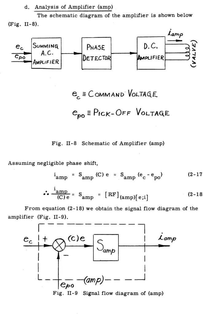
d. Analysis of Amplifier (amp)

The schematic diagram of the amplifier is shown below (Fig. II-8). "IN 41 N. 4 IT .. b %..I e COMM A ND VOLTAG F

ePO =PICK-OFF VOLTAQ.E

Fig. II-8 Schematic of Amplifier (amp)

Assuming negligible phase shift,

i _amp = Sam _amp (C) e

i

o* amp

(C)e

= Samp (ec -ePo_po Samp = [RF] (amp)[e;i]

From equation (2-18) we obtain the signal flow diagram of the

amplifier (Fig. II-9).

e-

omp

-Fig. II-9 Signal flow diagram of (amp)

(2-17) (2-18)

I~~

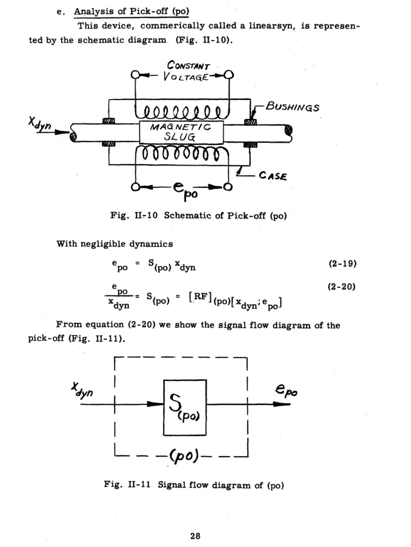
tor P F - - _ - - - .. Q net I I I

e. Analysis of Pick-off (po)

This device, commerically called a linearsyn, is

represen-ted by the schematic diagram.. (Fig. II-10).

CONS, AT

Fig. II-10 Schematic of Pick-off (po) With negligible dynamics

e po S(po) Xdyn (2-19)

e

Xdyn (po)

(2-20) = [RF] (po)[ Xdyn; epo]

From equation (2-20) we show the signal flow diagram of the pick-off (Fig. II-11).

F __ -

- -__

I-

-(p)

-Fig. II-11 Signal flow diagram of (po)

I I

I I

f. Analysis of Elevator Linkage System (els)

This is simply a linkage system for converting the linear

motion of the actuator into radial movement of the elevator at the

hinge line. The schematic diagram is shown in Fig. II-12.

dyb

Fig. II-12 Schematic of elevator linkage system (els) Let Sels

Then

= Linkage ratio of els

6e = Sels Xdyn (2-2 1)

(2-22)

and 6e _

-dy

= S

[ RF]

ri

Xdyn els

(els)[x;6]

Xdyn

From equation (2-22) we have the signal flow diagram of (els) (Fig. II- 13).

L

- -e

Is)

-Fig. II-13 Signal flow diagram of (els)

F--- -7

J

IC

I

g. Analysis of Entire Hydraulic Servo System (Ideal)

Combining the components of sections a through f, as indi-cated by Fig. II-1, the overall signal flow diagram is obtained in Fig. II-14. Using the relating functions of each component, as

prev-iously derived, the [RF] for the overall ideal hydraulic servo is

ob-tained as follows: [ RF (ihs)[ec; 61

[RF] (amp)[ e ;i][RF](v)[i;Q[RF] (as -eds) [Q;x[RF (els)[x ;6

1+ [RF] (amp)[e; i][RF](v)[i;Q][RF] (as-els)[Q;x] F1(els)[x;6] [RF(po)[x;e

(2-23) where: Sact ker

1

P Mnp +CdP+k + ka _{d e r a} [RF](as-eds)[Q;x] S k

1+[9

er

lF

P4jm

2+p

i

1+ _P [ _{P dp+ k +k} mp2+CdP _{_actk hyc d a}+k Lmp~.~C a er (2-24) Sact ker khyd

p[khyd (mp2+CdP+ke r+ka) _{+ ker(mp2+CdP+ka)}

Pjhyd~m rdpk 2

j

(2-25) Sact ker khyd

p[ m(khyd+ker)p +Cd(khyd+ker)P+khyd(k er+ka)+kerk (2-26)

Then:

[RF(ihs)[e ;6]

S S S S k k amp v els actker hyd

p[ mkp2+dkp+khyd(ke r+ka)+kerka

SpoSampSvSactkerkhyd

1+ _(2-28)

P [mkp2+Cdkp+khyd(ker+ka)+kerka]

amp Sv Sel8 Sact ker khyd

pmkp 2+ p+k k+k )+k k +S S S Skk

=

p[dp2 p+khy er+ka)+ker _{po ampSvSactker hyd} (2-29)

[RF] (ihs)[ec; 61

C~~~~~~~~~~~~~~~~~~~~~~~~~~~~

S _{amp v els act er hyd}55S S k k

mkp3_+Cdkp2_{+(khydker+k ka)P+SpoSampSvSactkerkhyd}

RelatingFunction of ideal hydraulic servo, for

command voltage in, elevator deflection out (2-30) For the simulation of the above equation, the reader is re-ferred to Chapter IV.

1-4 Co_to .Cd_C) la_O 0 (D_Co 1.4 Cd -. 0 4 "O_bO -I Cd 0 C) Co Cd 0)

0

I

I

I

to .f4

C. Analysis of the Nonlinear Hydraulic Servomechanism

Starting from the overall system block diagram (Fig. II-15),

each part is analyzed in turn.

Ne

Fig. II-15 Block Diagram of Nonlinear Hydraulic Servo.

a. Amplifier.

For our purposes, this is simply a sensitivity, with no

phase angle (as in ideal analysis). b. Valve.

For convenience, we assume balanced loads and balanced valves, and study only one half of the valve's hydraulic circuit.

Thus, the valve spool and cylinder may be "cut" in two, as shown in

Fig. II-16. D

Fig. II-16 Section of Valve

I

-Now, Qv = Q1 - Q2 and furthermore, Q1 and Q2 are dependent

upon the pressures across the orifices through which they flow.

is,

Q1 = kitA4P and likewise, _{Q2 = ki 17AP}

2

That (2-31) (2-32) where k is a constant, and i is current driving the solenoid.

These square roots are difficult to set up on an analog computer, so a means of approximation will be used. Remembering the balanced conditions of operation, we may draw an equivalent bridge circuit

(Fig. II-17).

PRESUR E

Fig. II-17 Valve Equivalent Bridge Circuit

The point D is at a pressure of Ps /2, where Ps is the supply

5

pressure, assuming Pr = _{0. Dropping the delta prefix on P}

1 and P2

we may express them in terms of Ps and PL where PL is the pres-sure exerted by the load due to interfering moments and load dynam-ics. ZAP1 = P1 = Ps - (Ps+PL) /2 = (PS-P) /2 (2-33) AP2 P = P - P1 = (Ps+PL) /2 kiNF s -Q1 = kli/(Ps-PL)/ 2 .. Q2 = k2i/ (Ps+PL)/2 Approximating, Q1 = kl i P s / 2 1- 2 Ps Q = k i _{Q= k} / P /_{2 Z 2NJ .1_ 1 l+L]P}

In general, _{Qno load} = ki f/PS/2

Therefore, if we':have the curves for Q1 and Q2 at no load, we may obtain the curves for load conditions as follows:

Fs.

(2 -40) (2-41) Q2 = Q2 no load Now, Qv = Q1-Q 2 ( 21 PL) Q2 S Qv [Qln. 1. (2-42) 1 PL n.l. Q2n. 1. ( _{2 P} S 1 PL -2n. 1. 2 P s 1n 2 _] (2-43) (2-44) so, and, I (2-34) (2-35) (2 -36) (2-37) (2 -38) , since PL =0 (2 -39) Q1 = Q1 no load I i 1 I l3 1 Q . Q .1 1+1 P

This may be obtained easily on the analog computer, as seen in Chapter IV.

c. Lines, Actuator, Mechanical System.

For convenience, we shall call this the linkage system,

since it connects the valve output to the elevator by means of fluid flow and mechanical linkages.

The relating function for this system will be written in

terms of Vv in, and xdyn out, for ease in instrumenting it later on_{v ~dyn}

the analog set-up.

[RF] (as-eds)= [RF ]linkage

-

rv

;

x,

(2-45)

-

V

UYI.L"-Sact ker khyd (2-46)

(2-46)' m(khyd+ke r )p + C d (k h y d+k e r)p + k a (k hy d + k e r )+ k e r kh y d

~~~~~~~~~~~~~~~~~~~~~~~~~~~~~~~~~~~~~~~ (For the derivation of equation (2-46), see section II-B. Also

see section II-B for obtaining Fdn )

Coulomb friction will be added when the actual computer

diagrams are considered (Chapter IV), since it is more conveniently

handled then than it is in equation form. d. Pick-off

This, as in the case of the amplifier, is simply a sensitiv-ity, with phase angle considered zero.

For simulation of the above, see Chapter IV.

CHAPTER III APPARATUS

It may be helpful to describe briefly the equipment used in the simulation carried out in this report. (All equipment to be discussed in detail was designed and developed by the MIT Instrumentation Lab-oratory, Analogue Computation Group.. ) The main piece of apparatus,

of course, is the analog computer itself, called the General Purpose

Simulator (GPS). Other items used include a master generator, two function generators, an electronic multiplier, a second order unit,

and assorted smaller units such as an oscilloscope, two limiters, and signal generators.

A. General Purpose Simulator

The simulator used in obtaining data for this report contains 7 integrators, 10 summing amplifiers, 21 potentiometers, and a num-ber of other features that enable one to simulate and solve differential equations of order as high as seven. Two of the aforementioned

po-tentiometers consist of two units ganged together, so that two para-meters may be varied simultaneously at identical values.. This

par-ticular feature was of great help in the present study, since the as-sumption of balanced values implies that the lap and leakage of one orifice equals the lap and leakage of the other.

The integrators have time constants which may be set as high

as 3000, so .that problems may be observed in real time units, as well

as in "slowed down" time.

B. Master Generator

output (Ovolts), and a calibrating line which may be displayed si-multaneously with the problem on the oscilloscope, so that quantity as well as quality of system response may be studied conveniently Another

feature of this generator is that it supplies a time reference. This is

obtained by connecting the generator's time dot intensity output to the "z" input of the scope; the scope's response trace (and the calibrating

line) is then illuminated at periodic time intervals (. 02 seconds in this study), so that time of response, etc., may be readily determined without reference to inaccurate grid overlays.

C. Function Generators

These were simply small electronic units designed for the

pur-pose of duplicating the sensitivity curve of any piece of equipment (in

particular, for duplicating hydraulic valve nonlinearities). Bias levets

may be set so that the operating level of the diodes within the function

generators are such that desired slopes and intercepts are obtained. D. Electronic Multiplier

This multiplier accurately multiplies two arbitrary functions,

and will also supply the sum and difference of the input quantities. The multiplier was very useful in simulating the effect of pressure feedback on the valve characteristics.

E. Second Order Unit

This unit supplies a second order lag adjustable to any desired

damping ratio and natural frequency. Its use obviates the effort and

complexity of wiring two additional integrators.

F. Other Equipment

No mention will be made of the other small units used in the

set-up, since their contribution to the overall problem is not important. For a view of the set-up used, see Fig. III-1. The GPS is seen

in the center. To the left is the electronic multiplier and to the right, placed above the master generator, are the oscilloscope and second

order unit.

For more detailed information regarding this equipment the reader is referred to the bibliography9_.

CHAPTER IV SIMULATION

A. Development of Numerical Constants

a. The actuator sensitivity is equal to the reciprocal of the area of the actuator piston, and can be defined as the derivative of the ratio of output displacement, Xact to fluid flow to the valve, Qact

Or

act2

Sact = pQat

]

1.81 in-2 (measured value). (4-1)

Sact P act

b. The elevator linkage system sensitivity is angular elevator' displacement per unit linear actuator displacement:

6e

Sels e 2.81 deg/in = 0.49 rad/in (4-2)

act

c. The actual elevator deflection would be (Selsxact) minus the loss due to system compliance which is a function of the force on the

actuator. Therefore:

6e = Sels act Sels SerAact 1 (4-3)

where Ser is the mechanical compliance of the linkage between actua-tor and elevaactua-tor, and i, is the pressure drop across the actuaactua-tor. Substituting Eq. (4-1) into Eq. (4-3), we have:

The flow to te actuator is the low out of tne valve less tne 1low loss due to compressibility of the fluid. In the static case where there is no flow from the valve:

S ~~~~~~~~~(4-5)

Qnet Qc Shyd P (4-5)

where Shyd is defined as

=AV

5

Shyd V in5/# (4-6)

(

Substitution of Eq. (4-5) into Eq. (4-4) gives:

{

r

6_{e el Sact hyd PL} + _{Sels er act PL}

PL Sels (Sact Shyd + SerAact) (4-7)

With the piston locked, the actuator, connecting rods, and ele-vator can be assumed to be a second order system with characteristic equation as follows. (Ip +c d p +k) 6e = 0 2 2 or k k ₌ 2 + _{1 (4-8)} ~~n

I c

_d

~ n

where n T (4-9)

k can be defined as the torque at the elevator hinge line due to an applied elevator deflection, 6

e , with piston locked:

Meh

k = eh (4-10)

e

The moment at the hinge line can be described by Fig. IV-1.

.. . . .. '' . ... - ..

VA TOR

£VA To R LŽ5F&"CT/cM/

Meh = Fr=Aact PL r

X

e r e (6e is small for locked piston)

6_{e x ( 1}

els x r r

.'. Meh Aact PL

Sels

Fig. IV-1 Schematic of Elevator and Hinge Line

Substituting the results of Fig. IV-1 and equation (4-7) into equation (4-10), we have:

AactPL els e

or,

Aact PI,

Sels [ P Sels (SactShyd + SeAact)

,. Aact

%

-

_els

S act

e

1 -I

Shyd + SerAact J

then from equations (4-9) and (4-12) Aact I Se1 2 Sact Shyd 1

+ SerAact

) or, since 1 Sact = Aact' APPIED _.1/ / /I&J (4-11) (4-12) (4-13) r I- -4-a V IN Y~~~~~~~ Wn - I I

Wn

1

2 (Sct

+

els (act Shyd

(4-14)

er

With the piston locked, a step displacement was applied to the elevator and the vibration of the elevator about its hinge line (with near zero damping) was recorded as 30 cps. With piston unlocked,

this vibration was recorded as 15cps. The first condition would cor-respond to Shyd = 0.

From equation (4-14) we have:

S 2 S + S 1

act Shyd + Ser 2 S 2

n els

2

Ielev. was known to be 1 100# in =

(4- 15)

2. 85#in sec2 so

Sac Shyd + Ser_{act hyd er} 1

an (2. 85)(0.49)2na

1.46 in - 2 #

n

(4-16)

With the actuator locked (i.e., Shyd 0), n 30cps and:

S = 1.46 = 4.12 x 10 5 in/# 5_{er in (9} (30x 22r)2

k

_er

- - =2.43x104 #/in

_S

(4

er

or 1-17) 1-18) With the becomes:

actuator unlocked, wn = 15cps and equation (4-16)

2act-5

Sact Shyd + _{4. 12 x 10-}

1.46 (15x27r) -2

Since Sact = 1. 81 in2 (see below)

Shy

hyd

d

[1

L

(1l5x27r)

2-

2

4.12xlO 5]

-

= 3.77x10 5 in5

420

(4-20) (4-19)

and

1 (_ _1 1 1 04

khy

1

1

_d

. 8x10_ #/in (4-21)

1~

~ ~

~ ~ ~ ~ ~~~~~~.1

f~ k = ~hhyd Sact 3. 77x10-5 _{o 1.81}

| _{The following constants were obtained by direct measurement:}

amp = 20 ma/volt -2 Sact

-Sct

= 1.81 in S _po = 3. 93 volts/ in Sels - .49 rad/in S = .587 in3/sec V l11d.

B. Simulation of Ideal Hydraulic Servo

The simulation of the ideal [RF] (ihs)[ec;6e] developed in Chapter II serves as an excellent illustration of the technique

employ-ed in simulating higher order differential equations. From Chapter

II, Section B, the above relating function is: [RF] (ihs [ ec ; ]

amp v act elskerkhd

3 2

~~~~~~~~~~~~~(4-22)

(4-22)

d + (khyd er k ka ) p + Spo amp SvSactkerkhyd

Using the values developed in Section A of this chapter, the

various coefficients above are calculated as follows (Cd and ka are to be retained as variable parameters):

Sam_amp p S S _{els act er hyd}Sact ker khyd =

v"* -"-'-sec.ma'"' -i m.

i..,.

~

n

v

= 22x108 #2/v-sec-i2 _(4-23)

= 22 x10 # fv-sec-in (4-23)

SampSvSactSpo ker khyd

(20 ma )(0.

V

i

i) 8m )22

2587

#

34

4 #

587 c )(3. 93 -)(1. 81 in- )(2. 52xlO )(0. 837xlO II-)

sec.ma in in in 2 = 176 x 108 sec - in (4-24) k=ker+khyd =2.52 x 10in +0. khyder+ k k_a 837x0 4 # = 3. 357xl 04 # in in (4-25) 4 #A14# ) = (2.52xl0 -)(0.837xl

_in

-)

_ina

+ (3. 357x104 ) ka = 2. 11x 108 + 3.357x10 4 k_a #smk = (0. ec684 )(3. mk = (0. 684 i )(3.

357xlu 4 )

in (4-26)

2.29x 10

4

_#2sec2

2 in (4-27) Cdk = 3. 357x 104 (ihs)[ ec; 6] [ 2.29xl 04p3+3. 3 57xlO4Cdp2+(2.11xl 08+3. 357x0lOa I a)p+176x108] 22x 104 2.29p3+3.357Cdp2+(2.11x10_p 4+3 357ka)p+176x104_~~~~~a S(ihs)[ 22x104 eC;6] 176x104 0.125 radV -1

.V

(4-29) (4-30) f I iI I Thus, [RF] #2sec Cd 2 in (4-28) 22 x 108 I . . . __

Sels S(ihs)[e ] -' S.--- '-rad 0.49 rad in 3, 93 --in 0.2rad V

From the above:

229-

dt

_{-13.357Cd~+(2.lxl}

+

dtdt

A357C4+(2x104+335 _{3.357k) +176xl 6 = 22x10e}04

(4-32) So that

2.29p 6=22xlO4ec-3_.3 5 7_{Cdp6-(2.xlO +3.357k )p6 -176x1046}

We can now draw a tentative simulator schematic, Fig. IV-2.

H/

Fig. IV-2 Tentative simulator diagram for ideal hydraulic servo

Check:

(4-31)

'I,

2

The loop gain of the actual equation is too high; in order to sim-ulate this equation, the time scale must be changed. Repalce p by

100 p, wo that the time dots on the computer's cathode ray

oscillo-graph (ordinarily 2 seconds apart) now represent 2 sec/100 = 0. 02 sec.

(Time is "slowed down"). With this new time variable, equation (4-33) becomes 2.29p36 =0.22ec-0.03357Cd2_{6(2.11+00003357ka)p6-176x10}4_{6 (4-34)} 29p 6= 2 c_ d a C C Further, let Cd = Cd (4-35) Cd - C _d -100 k k ref and k - a = 5 (4-36) a ka ref 105

Since the gain of potentiometers cannot exceed unity, amplifier gains may be employed to obtain the required numerical values for the con-stants. Fig. IV-2 then becomes Fig. IV-3(a).

Fig. IV-3(a) Final simulator diagram for ideal hydraulic servo

I /c - C c %

Since

V=

Q

C)

E]

; may be obtained from [RF] (Eq. 2-16)

as:

Expanding:

T~p2+

p

X=

V

dy

u

Also since V _{V7T ap} S [p]ec-Cp) _{r P)} it is seen that the above figure represents the ideal servo of Fig. II-14. Numerical constants in the

figure are time and scale factors. See Section A of this Chapter for parameter values.

Fig. IV-3(b) Final simulator diagram modified for ideal hydraulic serve

The above arrangement permits instantaneous observation of 6

(and its various derivitives ) as Cd, ka, and e are varied.

The preceding derivations serve to illustrate simulation

tech-niques; however, the simulator schematic as given in Fig. IV-3(a) should be modified for two reasons:

(1) Ease of parameter variation

(2) Facilitation of addition of nonlinearities

A modified schematic is shown in Fig. IV-3(b) which includes notes explaining the change.

C. Simulation of the Nonlinear Hydraulic Servomechanism

Once again, a piece-by-piece study is helpful, and the block

diagram for the system is repeated (Fig. IV-4).

Fig. IV-4 Block diagram of nonlinear hydraulic servo

a. Amplifier. The amplifier is represented on the analog by an inverter, coupled with a potentiometer for adjusting the gain. The amplifier also has its setting divided by imax, so that the output

is (i/i max), for reasons described later. (The factor 75 involves

m

imax

F

apl

-

j

| V Fig. IV-5 Analog of Amplifier

b. Valve. The valve on the analog computer is -composed of four sections: (1) two function generators which simulate the

es-sential transfer characteristics of the valve orifices, (2) one multi-plier which brings in the effect of pressure drop across the orifices

with increasing load, (3) an integrator to sum up the flow rate, giving a volume of flow out, and (4) a second order unit to account for valve dynamics.

The inputs to the function generators are non-dimensionalized, so that at zero lap the function generators have a gain of unity for large inputs. This unit slope facilitates readjusting the lap and leak-It . age after the sensitivity of the valve has been set to a new value. The

change in sensitivity is then accomplished by adjusting the setting of

the potentiometer in the amplifier analog circuit.

Lap and leakage must also be set on these function generators,

(

addition to the slope at low input currents. ~~~in By utilizing an elec-tronic multiplier, Qv is obtained, which is the flow under load con-ditions from the valve (Fig. IV-6).

L__

Fig. IV-6 Analog of valve

Lap is adjusted by feeding D. C. voltage (adjustable) into the function generator along with i/ima_max x . The leakage may be increased

or decreased by adding or subtracting a D. C. voltage from the output of the function generators. In the actual set-up used, the potentiom-eters were ganged so that lap and leadage could be set for both function generators A and B simultaneously.

Qv is supplied to an integrator, which yields Vv, the valve volume output. Also, a second-order unit is inserted into the input circuit to approximate the valve dynamics (due mostly to the hydraulic amplifier incorporated in the valve).

Dither is added by summing an alternating current with iimax

and applying the resultant current to the function generator.

c. Lines, Actuator, and Mechanical System. The analog

schematic is similar to that developed in the ideal case. (section B),

except that only two integrations are used, since the valve is assumed to have a volume output, rather than a flow rate (as was assumed in

The parameters for this second-order unit were obtained from direct frequency measurements of a typical valve (see Fig.IV-12A).

-_ - - - __ -_ - - __ -- I

I

.

Fig. IV-3(a) ). Also, coulomb friction is added here. (Fig. IV-7)

Fig. IV-:7 Analog of lines, actuator, and mechanical system

The inverter at the lower left hand corner of this diagram

ac-tually serves as a force summing member. The force this member

exerts on the actuator actually causes both the compression of the fluid and pressure drop across the orifices.

The equation represented above is as follows:

C

k-k

2 d a- hvdx

)

P Xdyn+ m1 02p xdyn m.104 dyn= 04 (aSa ctVv-x dyn)

I M-10 . M-1

(k hyd +k er()m4

-(4-37)

Cd k

but Fdy=m.1 Xdynm 20p Xdyn + 4 xdyn (4-38)

10 a0 I I I I I

F khdk

104yder(S V- (4-39)

4 4~~~~( act - dyn

(khyd+k)

10 (kactVv xd y n)

consequently Fdyn may be obtained conveniently from point "A" on

the diagram. Further refinements, as discussed in Section D, were later made in order to better approximate viscous friction effects,

and to relocate the pick-off.

Coulomb friction is simulated by first obtaining pxdyn on the

analog, This quantity is readily available as the output of the first integrator in Fig. IV-7. Now we want the coulomb friction to have a sign which will oppose motion, or expressed another way, we want it to have the same sign as the viscous damping term at the same

instant.

xdyn_/

Fcoulomb = C xdyn (4-40)

Xdynl

where C is a constant for a given system, in pounds of force. The quantity p xdyn (dy n) is amplified greatly, then clipped

at the value set for C. The resultant voltage represents

approx-imately the force exerted by coulomb friction upon. the force summing

member, for example, the actuator piston (Fig. IV-8)

+

C

C

L-I

Fig. IV-8 Coulomb friction exerted upon a body with sinusoidal motion

d. Pick-Off. This is represented by a potentiometer; no diagram is necessary. Dynamics in this device are neglected.

-I ~ D. Modifications of Original Simulator Circuit.

In the process of setting up the computer, it was felt that certain

modifications should be made to investigate the effects of friction at the actuator (as contrasted with the effect of friction at the elevator linkage). Also, it seemed worthwhile to try locating the feedback

pick-off at the actuator (rather than at the elevator linkage), thus

placing part of the system dynamics outside of the loop. The effect of this change on stability and system response time could then be evaluated.

a. Addition of Friction at Actuator. A simple sketch of the mechanical system from valve to elevator is shown in Fig. IV-9.

C.

r

lI

I-'

.

_-- I _{. -}

-

_/F I I

i~~cli

1 XQCF I Xdyn

Fig. IV-9 Mechanical system showing friction at actuator and elevator

In the above figure, point A represents the location of the ac-tuator, and point E represents the location of the elevator. The input

displacement is seen to be VvSact (The actuator sensitivity appears

at this point since the volume output of the valve must be converted to an equivalent displacement). With displacement in-displacement

nut the stiffrnas t'nVV0+0a1lq 1 ,k' I V % -I 1,%rgsc.ap ,-11 in

'

hyd"

merj'

a'

'L'L'6 "A' ^H - t~ l

pounds per inch, making the relative effects of these three constants more easily studied.

If~~

~With VvSact as an input displacement, it is seen that the force

1}~~~~~~~

I C V

r

1% iI iI I i I I i I i'I I i I i

exerted upon A by the hydraulic fluid is

Fhyd = khyd (Vv Sact - act) (4-41)

Tending to oppose motion is C the viscous friction damping coefficient at the actuator (point A)

FC = - Cd xact

The sum of these two forces, equations (4-41) and (4-42), (4-42)

is

Fhyd + FC khyd VvSact _{- v - Cd~~~~~~}X act (P C + khyd)

1

which must be balanced by the load forces transmitted through ker.

The load forces exerted at E are simply Fm + FC + Fk

a

_ Xdyn (mp + Cd2P + k_{a )} (4-44)

where Cd is the viscous friction damping coefficient

2

at the elevator, point E.

For equilibrium conditions, we must have Fhyd + FC

Cd 1

= - (F + FCd

d2

or, substituting the expressions for the various forces in equation

(4-45),

khydVvSact- act (PCdl + khy

1kyd

d ) = Xdyn(mP

We see also from Fig. IV-9 that

xdyn Xact - (compression _{dyn act} of k ~~er) xdyn = Xact Xdy_dynn (mp2 C k

_er

9, (4-43} + Fk ) a (4-45)

+ CdP

C2 + ka ) or, (4-46) P + ka) (4-47) II I

We now have two equations in two unknowns, act and Xdyn Combining equations (4-46) and (4-47) we have

khydVvSact-xdyn (1

d2

a2

m+C k p_{)(PCd +khyd) = xdy}

n(mP + Cd 2P+ka)

+r

ker

or, solving for xdyn/Vv

dyn Vv [(khyd+Cd p)(1t k _{hyd act}S mp +Cd P+ka 2 k zer )+(mp2 +Cd p+kd2 a

which may be expressed in better form as

kerkhydSact/ (khyd+ker+Cd

mp2+Cd P+ka+

2

(khyd+Cd P)ker

(1

To facilitate the addition of Cd to the existing analog wiring

1

diagram with a minimum of rewiring, we rewrite the numerator and the last term of the denominator of eqn. (4-49)

kerkhydSact khyd+k er+Cd p _[ hydker

. khyd+kJer

1 and (khyd+Cd 1 )ker khyd+ker+CdlP_.1 kh k - hyd er

i

Lkhyd+ker [1+ hyd (4-51) (4-48) xdy V v (4-49) 1 i Sact (4-50) I ifI i II

Equation (4-50) indicates that a first-order lag,[ I 1

Cdp

+ 1hyder hyd er must be inserted in series with the potentiometer representing

kerkhyd ₎

er +khyd in the analog circuit. Equation (4-51) shows that the only

other circuit modification is the addition of a first order lead;

CdlP 1+ k1

khyd , in the direct connection between xdydynn and summing amp-lifier R in Fig. IV-10. As seen from this figure, the first order lead

was formed by merely.leaving the direct connection to amplifier R (thereby feeding xdyn into R), obtaining PXdyn at another point in the

Cd

circuit, multiplying it with a potentiometer by( k 1 and finally

hyd C P

connecting that signal to amplifier R (thereby feeding ( 1 ) into R). hyd

The resultant signal coming out of summing amplifier R, neglecting a sign change, is then

CdP

Xdyn ( 1+ 1

khyd

b. Relocation of Pick-Off at Actuator

From equation (4-47) we have

1 +

Xact = Xdyn + kr(mp Xdyn+Cd2 PXdyn +kaXdyn)

It is seen. that the quantity A in Fig. IV-10 is

A = - (mp Xdy(pXdynn +Cd P dyn +ka Xdyn

therefore Xact = Xdyn

i,

39 A

ker

Fig. IV-10 Modified analog of lines, actuator, and mechanical system Xact is thus easily obtained from summing amplifier S as shown.

(Numerical factors refer to scaling, which will not be discussed here. ) Fig. IV-11 is a schematic of the final simulator set-up. Potent-iometer, integrator, and amplifier designations refer to the actual

GPS computer used; Fig. IV-12 gives the frequency response and av-erage leakage characteristic of a typical hydraulic valve.

c.) Cd ea) 0 -l Cd A "-4 o. i *-I o-4 I p 6 i I I z ,I I[

a; -in o C) os,-I_Fq 4 d X 4-X

0>

'

0 V) 0 14 a)~~~~~~~ ( /

L

)

C

)

'4 ~ ~ C.. a)

Lt)

tb lh~~ _7 It Rp Cd~(L 1 14~~~~~~ a) ,-A a) a)bED a) U) a) Cd a ) *a) *1-0Z>c1v

~~~~~~~~~~~~~~~~~~~~~~~~~~~~~~~~~~~~~~~~~~~~~~~~~~~~~~JI--

Z

-\ z

I

co

"

N1 I (1) - I I I _A-A LfL0 _{- -} %"I

CHAPTER V DATA

A. Ideal Hydraulic Servo

Figs. V-1, (A-4, are photographs of various responses obtained

for an "ideal" servo (i. e., one whose valve characteristic is given by Qv = kiamp ); the pick-off is placed at the elevator and the actuator

contains no viscous damping. The system is as represented in Fig. IV-3(b), with all constants as calculated in Chapter IV except for the following parameters which were varied:

1) Sv amp Sact

Sref , where Sreref f = 100

C 2) d , where Cd Cd ref

ref

k 3) a oJk_a aref

, where

ka

ref = 1000 = 10, 000

With this system, optimum response time (measured as

0. 056 secs) was obtained with SvS a m Ppa ct

Sref = 0.1, _Cdrefd = 0.088 k

and a = 0. 05. Values of these parameters selected for response

aref ref

study are:

SvSamp act = 0.4, 0.088, and 0.2

ref Cd Cd = 0.03, 0.1, and 0.4 dref k a k aref = 0.05, 0.30, and 0.60 , k with ka aref aref

the variable on each photograph. hold for each photograph (highest values sponse curves of greatest damping):

SvSampSact Cd

ref ~

C

d

Photo A) B) C) D) E) F) .04 .04 .04

The following conditions k of a

aref

correspond to re-k_a k

aref

.05 .30 .60 rer 03 .10 .40 .088 o 088 . 088 . 03 .10 . 40 05 . 30 60 . 05 30 * 60 05 30 60 .05 . 30 60 05 o 30 . 60 ~m

m U C) (n 0 en S L) U) En -:>

4-' 0C. -I Q) U1) 0 U) a) U, a) rX4

-4 0 c-) (U) i) 0ut a) 4-h U) U) 0_u~ -4_ul e-4 -e4

4-0o 0 ! 4- 4 -0 -4 .- 4 *4h U) Y C)Q C) > ^ ¢ C). · ~- .O~.-b0

0q

o o~ 44-I 0 Q C) 4--~~~~~~.-U1 -4 _CdUCd -> U ) *~O C° U 0. . 0 -4 . E CU _o~ * -o .4~U) U)~~~~~-0 a) s od .

--S --S _{v ampSact} S C _d k_a

S C IF

Sref

_Cdref

ka

_ref

Photo G) .20 .03 .05 30 .60 H) .20 .10 .05 .30 . 60 I) .20 .40 .05 .30 .60

J) Step Input of 2 volts for all the above responses. B. Nonlinear Hydraulic Servo (Pick-Off at Actuator)

Fig. V-2 is a photograph of a typical "valve characteristic" as generated by the function generator used to obtain the nonlinear data that follows.

Figs. V-3,(A-DD)are photographs of the various responses ob-tained for a nonlinear servo; the pick-off is now placed at the actuator

(and hench, elevator dynamics are not included in the closed loop), viscous damping is present at both the elevator and actuator, and cou-lomb damping has been included. Dither has been neglected since its

effect was observed to be negligible. This may be explained on the

basis of the fact that a balanced valve is considered in this problem. The system is as represented in Fig. IV-1 1. The following quantities were varied:

1) Pressure feedback (i. e., the effect of load upon the

differen-tial orifice pressure) under differenc aerodynamic loads;

valve settings were zero lap and .02 leakage.

2) Aerodynamic load with different valve leakage and laD

Dara-meters.

3) Aerodynamic load with various coulomb and viscous damp-ing values. (Valve set at . 04 leakage and. 2 underlap).

4) Magnitude of step input under different aerodynamic load

and valve conditions. !

5) Aerodynamic load with several valve underlap and leakage conditions.

6) Aerodynamic load with different elevator inertias and valve

underlaps (Leakage set at .02). l

7) Aerodynamic load with different valve underlaps (Viscous i

friction lumped at the actuator).

8) Aerodynamic load with different valve underlaps (With

inter-fering moment at the elevator).

With reference to (1) above where the pressure feedback value of 49 is the calculated potentiometer setting; the command voltage was a step of 1. 18 volts. The higher pressure feedback values

cor-respond to the smoothest or most highly damped responses:

k/k

Pressure Feedback

aref Photo A) 0 0 .49 B) .05 0 .49 C) .30 0 .49 0~~~~~~~~~~~~~~~~~~~~~~ D) .60 0 .49

With reference to (2) above with a command voltage step of 1. 18 volts; increasing the load in each case smooths or dampens the response:

U C) 0 0._M U) a) 41 En En S 0) 14 0 0

z

m Wi *-4

aS w 0 C) -u) a) 0 04_v) a) CN_u 4 a) -4A_U) * -4_Cd a) *r. 0

z

b!

0 0 U) 0i) 0 4. U) 5 .9-4 '-4 C 0 z .- 4 r34

-r.

u~ 0 ta U)_o a) 4 U)

.i-I_I.4LO)

C a) 0 z 0

z

U) H-4 0 u c) 0_tQ 04 a} En 4-U) Fat (e *- | ;'4

0 U1 0 u U) (n 0 U)₀ 0) ~l Z_U) Ui) CU ! a> 0 -b

4e1¢ . 0 c) U) 0o_us U) I8_0. in 0) oP-I © ol 0)_r. -) 0 z co bB N

U 0 0 k_c)m m-02 0o_CL ! 0>_a) 4J m 02 02 5.4 cd *-6 0 .- 4 Nz

ka/ka

aref Photo E) F) G) H) 0 .05 .30 .60 0 . 05 . 30 . 60 0 .05 . 30 .60 0 .05 .30 . 60 0 0 ,04 ..04 0 .2 0 .2

With reference to (3) above with a measured frictional ele-vator hinge moment of 111 in.-lbs. corresponding to a voltage of

. 743 volts applied at the first integrator in the mechanical circuit;

the command voltage was a step of 1. 18 volts. The addition of cou-lomb damping in each case dampens the response:

#sec)

kaAe Cd = Cd #c se)Coloumb damping

41aefa d1 2 (volts)

ref

Photo I) 0 50 .743 0 J) .3 50 .743 0 K) 0 25 .743 0 L) .3 . 25 .743 0

With reference to (4) above with viscous damping values of

5#sec.

50 #sin; the highest vali"e of step input corresponds to the highest final response in each cae

final response- in each case.: