An inventory of methods for estimating climate change-informed design water levels for floodplain mapping

(1)

Publisher’s version / Version de l'éditeur:

Vous avez des questions? Nous pouvons vous aider. Pour communiquer directement avec un auteur, consultez la première page de la revue dans laquelle son article a été publié afin de trouver ses coordonnées. Si vous n’arrivez pas à les repérer, communiquez avec nous à [email protected].

Questions? Contact the NRC Publications Archive team at

[email protected]. If you wish to email the authors directly, please see the first page of the publication for their contact information.

https://publications-cnrc.canada.ca/fra/droits

L’accès à ce site Web et l’utilisation de son contenu sont assujettis aux conditions présentées dans le site LISEZ CES CONDITIONS ATTENTIVEMENT AVANT D’UTILISER CE SITE WEB.

Technical Report (National Research Council of Canada. Ocean, Coastal and River Engineering), 2019-03-29

READ THESE TERMS AND CONDITIONS CAREFULLY BEFORE USING THIS WEBSITE. https://nrc-publications.canada.ca/eng/copyright

NRC Publications Archive Record / Notice des Archives des publications du CNRC :

https://nrc-publications.canada.ca/eng/view/object/?id=d72127b3-f93b-48fb-ad82-8eb09992b6b8 https://publications-cnrc.canada.ca/fra/voir/objet/?id=d72127b3-f93b-48fb-ad82-8eb09992b6b8

NRC Publications Archive

Archives des publications du CNRC

For the publisher’s version, please access the DOI link below./ Pour consulter la version de l’éditeur, utilisez le lien DOI ci-dessous.

https://doi.org/10.4224/40001231

Access and use of this website and the material on it are subject to the Terms and Conditions set forth at

An inventory of methods for estimating climate change-informed design water levels for floodplain mapping

(2)

An Inventory of Methods for Estimating

Climate Change-Informed Design Water

Levels for Floodplain Mapping

Report No.: NRC-OCRE-2019-TR-011

Date: March 29, 2019

Author: M.N. Khaliq

Ocean, Coastal and River Engineering Research Centre

(3)

ISBN 978-0-660-30536-3

(4)

Acknowledgements

The work reported here was undertaken within the framework of an inter-departmental agreement between Natural Resources Canada (NRCan) and the National Research Council Canada (NRC). Project co-ordination support from Monica Harvey, from the Climate Change and Adaptation Division of NRCan, and leadership of Mary-Ann Wilson from the same Division is much appreciated. Partial funding for this project came from the Marine Infrastructure, Energy and Water Resources (MIEWR) program of the NRC, which is graciously acknowledged. Enzo Gardin of the NRC provided the much needed contract development support. Review comments from Andrew Cornett, Program Leader of the MIEWR program helped improve the description of various methods reviewed and overall quality of the report. Contributions from Saeideh Kheradmand of NRC/University of Ottawa are much appreciated. Review comments from five anonymous reviewers, designated by NRCan, helped improve this report further.

The information provided in this report is expected to help the engineering consulting community and other professionals involved in climate change impact analysis and decision-making in general and more specifically for flood mapping purposes. The contents are of guidelines nature, representing present state of the knowledge, and should therefore be updated regularly as the adaptation needs of floodplain maps may evolve over time in response to

changing climate conditions and also to conform to new knowledge from the climate science and engineering communities.

(5)

Executive Summary

The federal government of Canada has created the National Disaster Mitigation Program (NDMP) led by Public Safety Canada (PSC) with guidance from Natural Resources Canada (NRCan). The objective of the NDMP is to reduce the impacts of natural disasters in Canada by focusing government investments on recurring floods. For implementation of the NDMP, four domains of interest have been identified by PSC/NRCan – (1) risk assessment, (2) flood mapping, (3) hydrology and hydraulics, and (4) climate change. Through a collaborative inter-departmental agreement, the National Research Council Canada (NRC) – Ocean, Coastal and River Engineering Research Centre (OCRE) was retained to prepare an inventory of methods used for estimating climate change-informed design water levels for floodplain mapping in riverine and coastal environments. This effort is concerned with the above mentioned fourth domain of interest and thus will inform the development of national principles, best-practices, and guidelines on flood mapping for the NDMP. The initiative of developing new guidelines and best practices is being led by NRCan, with support from many federal and provincial

government departments and engineering consulting community. The goal of modernizing Canada’s flood maps is to reduce the adverse impacts of flooding on humans, the environment, cultural heritage, social and economic activities, and new development opportunities as Canadian communities flourish.

For floodplain mapping in riverine environments, statistical frequency analysis is performed on high river flows to obtain a set of design flow values corresponding to selected frequencies of occurrence, commonly interpreted in terms of return periods or annual exceedance probabilities (AEPs). For urban settings, the same statistical approach is used to develop precipitation

intensity-duration-frequency estimates, which are then integrated with urban hydrological models to produce desired design flow values. The estimated design flows are then used in hydraulic models to generate flood extents and levels for the creation of flood inundation, flood hazard and other flood related maps and products. These maps and products are useful for developing flood risk metrics, residential and industrial insurance guidelines, new development plans, and to inform communities about possible flooding scenarios and associated risks. For coastal environments, design water levels are obtained through a suitable combination of various wave characteristics, wave run-up and storm surge elevations. The estimates of desired design water levels corresponding to selected AEPs are obtained using conventional statistical

frequency analysis or joint frequency analysis approaches. The latter is a relatively new

emerging technique. Irrespective of coastal or riverine settings, the estimated design water levels are generally based on historical observations, assuming a stationary climate. It is also assumed that the design water levels derived from historical observations will also be applicable for future periods. However, with the world’s climate projected to change as documented in a series of Intergovernmental Panel on Climate Change (IPCC) reports, these estimates will no longer be representative of future conditions. Therefore, appropriate provisions for climate change need to be considered when developing floodplain maps. There are myriads approaches for

(6)

accomplishing this task and all of the approaches differ from each other in complexity, accuracy, physical relevance, and ease of use. The differences between approaches are driven mainly by the way climate change projections are developed and integrated with impact models, for example hydrological models.

This report presents a review of various approaches that have been developed, proposed or are considered suitable for Canadian conditions to incorporate the effect of climate change on design water levels for developing floodplain maps. To complement this effort, a short review of similar international approaches has also been incorporated. Most of these approaches rely on

projections from Global Climate Models (GCMs), which are the primary tools that climate scientists use to study climate change, and have been used to generate climate data to support IPCC reports (e.g. CMIP3 and CMIP5 simulations). Five major assessment reports have been generated by IPCC, with the most recent report released in 2013. The output from GCMs is subject to various types of uncertainties. For example, GCMs tend to underestimate the variance and persistence noted in observations, and consequently, are thought to generally underestimate climate extremes, which has important implications for design engineers and water resource professionals. According to the IPCC, the uncertainty of projections increases as the planning horizon increases with scenario-related uncertainties dominating other types of uncertainties. However, some investigators have found slightly different results. Tens of thousands of highly trained, independent scientists around the world collect and analyze climate data and develop models of global and regional climate change, which are typically tested using historical data and projected into the future, to support IPCC’s work (IPCC, 2007).

Following a brief introduction in Chapter 1, Chapter 2 of the report presents a general

introduction to climate change and the tools and approaches required to study climate change across multiple spatial and temporal scales, along with short descriptions of climate change scenarios and associated uncertainties. This information was necessary to establish a firm basis for the inventory of methods presented in Chapters 3 and 4, mainly because specialized climate scenario related terminology is frequently used in these chapters. Specifically, Chapter 3 deals with the inventory of methods for estimating climate change-informed design water levels for riverine and urban settings. Chapter 4 presents a similar review as in Chapter 3, but is focused on methods used for coastal environments. A set of thoughtful guidelines is detailed in Chapter 5 to support floodplain mapping studies, specifically from climate change related perspectives. A synthesis of the overall review of various methods discussed in the report and a set of potential recommendations are provided in Chapter 6.

(7)

List of Figures

Figure 1: NRCan’s roadmap for quantitative inclusion of climate change into floodplain

mapping. Source: Sub-Group on Climate Change, Natural Resources Canada. ...5 Figure 2: Projected changes in (a) average global surface temperature and (b) average

precipitation, derived based on CMIP5 GCM simulations, for the 2081–2100 with respect to the 1986–2005 period for two Representative Concentration Pathway (RCP) scenarios. The number of models/simulations used to derive these results is shown at the top right side of each panel. Stipulated areas show regions where at least 90% of the models agree in the sign of change. Figure adapted from IPCC (2013). ...7 Figure 3: Maps of observed precipitation change over land from 1901 to 2010 (left-hand panels)

and 1951 to 2010 (right-hand panels) from the Climatic Research Unit (CRU), Global Historical Climatology Network (GHCN) and Global Precipitation Climatology Centre (GPCC) data sets. Trends in annual accumulation have been calculated only for those grid boxes with greater than 70% complete records and more than 20% data availability in first and last decile of the period. White areas indicate incomplete or missing data. Black plus signs (+) indicate grid boxes where trends are significant (at the 90% confidence interval). Source: IPCC (2013) Supplementary Material. ...8 Figure 4: Annual mean changes in runoff and soil moisture for 2081–2100 relative to 1986–2005

under the RCP8.5. The number of Coupled Model Inter-comparison Project Phase 5

(CMIP5) models to calculate the multi-model mean is indicated in the upper right corner of each panel. Hatching indicates regions where the multi-model mean change is less than one standard deviation of internal variability. Stippling indicates regions where the multi-model mean change is greater than two standard deviations of internal variability and where 90% of models agree on the sign of change. Source: IPCC (2013). ...9 Figure 5: A schematic diagram of climate downscaling to drive impact models for climate

change studies at local and regional scales (adapted and modified from Khaliq, 2018). Abbreviations are described in the text. ... 13 Figure 6: A conceptual depiction of different sources of uncertainties associated with climate

model projections. The abbreviations used in the diagram are: GCM–Global Climate Model; RCP–Representative Concentration Pathway; RCM–Regional Climate Model; SD–

Statistical Downscaling; PS–Parameter Set. ... 19 Figure 7: (a) Flood hazard map for Badger, NL (source: Water Resources Management Division,

Department of Municipal Affairs and Environment, Government of Newfoundland and Labrador) showing flood hazard zones corresponding to 20-year and 100-year flood flow inundation levels. (b) Flood hazard map of Calgary, AB (source: Alberta Environment and Parks, Government of Alberta) showing flood hazard zones corresponding to floodway (where velocity is ≥ 1 m/s and depth is ≥ 1 m) and flood fringe (where velocity is < 1 m/s and depth is < 1m). ... 20 Figure 8: Floodplain map showing spatial patterns of flood depth corresponding to100-year flood

(10)

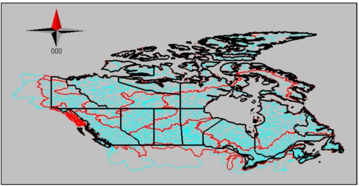
Department of Municipal Affairs and Environment, Government of Newfoundland and Labrador. ... 21 Figure 9: Division of Canada into large and small drainage basins on a map of scale 1:1 million.

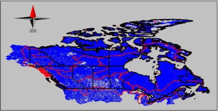
... 24 Figure 10: Canadian map showing large drainage basins and stream segments on a map of scale

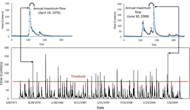
1:1 million. ... 25 Figure 11: Demonstration of extracting annual maximum and peaks-over-threshold (POT)

samples from daily flow time series of Little Pic River near Coldwell, ON for the 1973 to 2011 period (bottom panel). Top two panels show daily flow hydrographs for the years 1976 (left panel) and 2008 (right panel). In simple terms, POT sample will consist of all values exceeding 100 Cumecs (m3/s) threshold. ... 27 Figure 12: Block diagram of atmospheric inputs and typical landscape processes involved in

runoff generation in a watershed, showing the complex nature of nonlinear input-output relationships (structure modified from Arthur and Safer, 2019). The hydrograph at the outlet of the watershed is the net result of all of these processes that are working simultaneously at different spatial and temporal scales. In the diagram, notations T, ET, P, S and Q

respectively stand for temperature, evapotranspiration, precipitation, storage and discharge. ... 28 Figure 13: Integration of climate projections with impact modelling framework for floodplain

mapping. Arrows of different colours demonstrate flow of information from various

component processes. ... 30 Figure 14: Environment and Climate Change Canada’s precipitation IDF relationships for four

selected locations (Kirkland Lake, Ottawa CDA and Pierre Trudeau Airport). ... 46 Figure 15: A generalized process diagram for coastal flood risk mapping for historical and future

(with appropriate projections of various components involved) conditions. Arrows of different colours are used to demonstrate flow of information from various component processes. ... 59 Figure 16: A generalized framework for generating climate change-informed design flows and

water levels for floodplain mapping in riverine and urban environments... 76 Figure 17: A step-wise summary of the proposed framework for undertaking a climate change

(11)

List of Acronyms

Acronym Description

ACASA Atlantic Climate Adaptation Solutions Association AEP Annual Exceedance Probability

AR4 Fourth Assessment Report

AR5 Fifth Assessment Report

BCCA Bias Correction Constructed Analogues

BCCAQ Bias Correction Constructed Analogues with Quantile Mapping Reordering BCSD Bias Corrected Spatial Disaggregation

BR Beta Regression

CAF Canadian Armed Forces

CCA Canonical Correlation Analysis

CD Chart Datum

CI Climate Imprint

CIRNA Crown-Indigenous Relations and Northern Affairs CLASS Canadian Land Surface Scheme

CMIP3 Climate Modelling Inter-comparison Project Phase 3 CMIP5 Climate Modelling Inter-comparison Project Phase 5 CRA Conestoga-Rovers and Associates

CRCM Canadian Regional Climate Model CRD Capital Regional District

CRU Climatic Research Unit

DRDC Defence Research and Development Canada GHCN Global Historical Climatology Network ECCC Environment and Climate Change Canada

FBC Fraser Basin Council

FCL Flood Construction Level

FEMA Federal Emergency Management Agency FMC Federal Flood Mapping Committee FWHA Federal Highway Administration

GCM Global Climate Model

GD Geodetic Datum

GeoHMS Geospatial Hydrologic Modeling System

GEV Generalized Extreme Value

GHGs Greenhouse Gases

GIS Geographic Information System

GLM Generalized Linear Model

GPCC Global Precipitation Climatology Centre

HBV-EC Hydrologiska Byråns Vattenbalansavdelning-Environment Canada HEC Hydrologic Engineering Centre

HHWLT Higher High Water Large Tide HRM Halifax Regional Municipality

HSPF Hydrological Simulation Program - FORTRAN IDF Intensity-Duration-Frequency

(12)

IPCC Intergovernmental Panel on Climate Change KNN-WG K-Nearest Neighbor Weather Generator

KR Kernel Regression

KWL Kerr Wood Leidal

LARS-WG Long Ashton Research Station Weather Generator LiDAR Light Detection and Ranging

MEB-WG Maximum Entropy Bootstrap Weather Generator MIEWR Marine Infrastructure, Energy and Water Resources

NARCCAP North American Regional Climate Change Assessment Project NCEP National Centre for Environmental Prediction

NDMP National Disaster Mitigation Program NHC Northwest Hydraulic Consultants

NHMM Nonhomogeneous Hidden Markov Model NRC National Research Council Canada NRCan Natural Resources Canada

NWSRFS National Weather Service River Forecast System OCRE Ocean, Coastal and River Engineering

PCA Principal Component Analysis PCIC Pacific Climate Impacts Consortium

PCSWM Personal Computer Storm Water Management Model

POT Peaks-Over-Threshold

PRECIS Providing Regional Climates for Impacts Studies

PS Parameter Set

PSC Public Safety Canada

RAS River Analysis System

RCM Regional Climate Model

RCP Representative Concentration Pathway

SSARR Streamflow Synthesis and Reservoir Regulation

SD Statistical Downscaling

SDSM Statistical Downscaling Model

SHE Systeme Hydrologique Europeen

SLR Seal-Level Rise

SRES Special Report on Emissions Scenarios

STARDEX Statistical and Regional Dynamical Downscaling of Extremes for European Regions

SWMM Stormwater Management Model

TLFN Time-Lagged Feed-Forward Neural Network UBCWM University of British Columbia Watershed Model USACE US Army Corps of Engineers

VIC Variable Infiltration Capacity

WG Weather Generator

(13)

1 Introduction

1.1 Background

The federal government of Canada has created the National Disaster Mitigation Program (NDMP) led by Public Safety Canada (PSC) with support from Natural Resources Canada (NRCan) (https://www.publicsafety.gc.ca/cnt/mrgnc-mngmnt/dsstr-prvntn-mtgtn/ndmp/index-en.aspx). The main objective of the NDMP is to reduce the impacts of natural disasters in Canada by focusing government investments on improved floodplain modelling and delineation in order to reduce social and economic damages caused by recurring floods. As stipulated by PSC, this target will be achieved by modernizing Canada’s floodplain maps based on new technological developments, new analysis tools and improved scientific understanding of hydrologic investigations, hydraulic modelling and future climate change, as well as by developing refined geospatial data sets. To support this initiative, a comprehensive review of international and national hydrology and hydraulic guidelines for floodplain mapping was compiled by the National Research Council Canada (NRC) in Khaliq and Fergusson (2016), and that of flood frequency analysis procedures and two-dimensional hydraulic modelling tools in Khaliq (2017) and Khaliq and Piche (2017), respectively. For large lake and coastal settings, a review of high water level modelling and estimation procedures was gathered by the NRC in Murphy and Khaliq (2017). These studies were conducted through inter-departmental

agreements between NRCan and the NRC. Some of the related information is taken directly from these sources to complement the work presented in this report, which is prepared within the framework of another inter-departmental agreement between NRCan and the NRC.

For floodplain delineation and modelling studies, both for riverine and coastal settings,

information on design water levels (corresponding to certain low exceedance probabilities, e.g. 1%, 0.5% or 0.2%, etc.) is generally required. For riverine settings, this information is derived mostly through hydrological investigations combined with hydraulic modelling. The

hydrological investigations pertain to the study/analysis of the rainfall-runoff component of the hydrologic cycle, especially the peak flow values and use of statistical frequency analysis

techniques to obtain design flow estimates at various points of interest within a study region. For urban areas this information is based on precipitation intensity-duration-frequency estimates and urban hydrological model outputs for the area of interest. For coastal settings, information on design water levels is obtained by analyzing various wave characteristics, wave run-up and storm surge elevations. Conventionally, all of the above analyses and investigations are performed using observed historical data or various model outputs assuming a stationary climate. Due to climate change as projected by Global Climate Models (GCMs) and documented in various reports of the Intergovernmental Panel on Climate Change (IPCC) (IPCC, 2007, 2013), the assumption of a stationary climate has become questionable and therefore the applicability of design water level indices, derived from historical observations, has also become questionable. To help account for the effect of future projected climate change on design water levels for

(14)

floodplain mapping, scientists have proposed specific modelling techniques, analysis

frameworks, mitigation and retrofitting approaches, and broad recommendations. This report is focused on the review of various methods, available in Canada, for estimating climate change-informed design flows and water levels for floodplain mapping purposes. Additionally, to provide a broader perspective on this subject, selected internationally proposed approaches have also been reviewed. It is worth pointing out that many human related activities clearly affect the climate system. Most importantly, emissions of greenhouse gases, especially carbon dioxide and methane, are causing more heat to be trapped within earth’s atmosphere. Therefore, the case for significant climate change is compelling in both the empirical observations as well as theoretical predictions. A warmer air mass can hold more water (i.e., warmer air has a higher saturation vapor pressure). Therefore it is reasonable to expect higher amounts of water vapor in the air, leading to intensification of the hydrologic cycle, with impacts ranging from one region to another and from one component of the hydrologic cycle to another.

The Federal Flood Mapping Committee’s (FMC) “Sub-Group on Climate Change” has

developed a preliminary framework, named roadmap (see Figure 1), for incorporating the effect of climate change on floodplain maps in order to support various objectives of the NDMP. The FMC is being led by NRCan and PSC, with members from various federal government

departments, including ECCC (Environment and Climate Change Canada), CAF (Canadian Armed Forces), DRDC (Defence Research and Development Canada), NRC, CIRNA (Crown-Indigenous Relations and Northern Affairs), and INFC (Infrastructure Canada). The Sub-Group on Climate Change includes members from ECCC, Government of Alberta and NRCan. The Sub-Group on Climate Change: (i) provides advice on climate change and floodplain mapping for the FMC, (ii) supports the development of “Federal Floodplain Mapping Guidelines Series” documents, (iii) supports projects that improve the understanding of how climate change affects flooding and floodplain mapping, (iv) engages in consultation activities with other stakeholders and practitioners, and (v) shares information sources, references and relevant projects with all interested parties (Harvey, 2018).

The roadmap was developed following the recommendations that emerged from NRCan’s Workshop on “Climate Change and Floodplain Mapping”, held in Edmonton on March 20 to 21, 2018 and a number of follow up discussions. The review of various methods presented in this report is expected to support various component tasks of this roadmap. For a given situation, a specific method or a combination of different methods can be used to incorporate the effect of climate change into floodplain mapping procedures.

To set the stage for developing climate change informed floodplain maps, a considerable portion of this report is devoted to reviews of climate downscaling and climate change impact

assessment approaches, specifically with reference to estimating climate change informed design flows and water levels for floodplain mapping. In this review, the emphasis is on various

(15)

often used for estimating design flows and water levels. The inclusion of this information was considered necessary since specialized climate and scenario-related terminology has been

frequently used throughout the report. With this information included, the report can be read as a standalone document.

1.2 Objectives

The objectives of this study were to compile the following information:

 An inventory of the methods for estimating climate change-informed design (flood) flows or water levels for floodplain mapping in riverine settings, along with methods for estimating design water levels for urban environments;

 An inventory of the methods for estimating climate change-informed design water levels for floodplain mapping in coastal settings; and

 A synthesis of the reviewed methods to support NRCan’s roadmap for quantitative inclusion of climate change information into floodplain mapping, which, in turn, will inform the development of national principles, best-practices, and guidelines on floodplain mapping in support of the NDMP.

1.3 Organization of the Report

This report is divided into six chapters, including this introduction chapter, and a section on references. An introduction to climate change, climate modelling, emissions scenarios, and downscaling methods is provided in Chapter 2 in order to provide the reader with sufficient background on these topics for developing climate change informed design water levels. Chapter 3 of this report provides a review of various methods used/developed for incorporating the impact of climate change on estimating design flows and water levels for floodplain mapping in riverine settings. This review also considers methods used for estimating precipitation intensity-duration-frequency analyses, which are often integrated with urban runoff estimation models. Chapter 4 presents a similar review as given in Chapter 3, but for coastal settings. This latter review considers mainly the characteristics of waves, wave run-up levels, tides and storm surges used for estimating design water levels for floodplain mapping. Chapter 5 presents a generalized framework to support initiation of a floodplain mapping study, mainly from the perspective of incorporating climate change. Chapter 6 presents an overall synthesis of the review and discusses potential recommendations for updating existing floodplain maps and steps necessary to be followed for undertaking new flood mapping studies, with the inclusion of climate change information. A list of references cited is available at the end of the report.

(16)

The reviews and discussions provided in this document are intended for use by individuals that have some basic understanding of flood-producing mechanisms in riverine and coastal settings, methods pertaining to floodplain analysis and statistical theory involved in the estimation of design floods and water levels, specifically for floodplain mapping purposes. The documents and information sources considered for this report are those which are related to the methods

reviewed and are available in public domain or through dedicated periodicals related to engineering and sciences, as well as those related to climate change science. Where required, references are also provided for obtaining additional information and details on reviewed

methods. The focus of the review is mainly on Canadian studies. However, a selective review of similar international studies is also included in order to provide a broader perspective on the subject. By no means does this report present an exhaustive review of all of the methods available for incorporating the effect of climate change in floodplain mapping procedures. In addition, this report does not evaluate sources of uncertainty associated with the underlying data sets for each reviewed method and it also does not attempt to present feature-to-feature

comparisons of reviewed methods, advantages and disadvantages. Descriptions of various theoretical aspects that underpin reviewed methods are outside the scope of this report. For such descriptions, technical/scientific articles and reports associated with these methods can be referred to. Information on these sources can be found in the references section of the report.

(17)

Figure 1: NRCan’s roadmap for quantitative inclusion of climate change into floodplain mapping. Source: Sub-Group on Climate Change, Natural Resources Canada.

(18)

2 Climate Change, Climate Downscaling and Climate

Projections

2.1 General

Climate has been changing over multiple time scales and therefore climate change can be defined in numerous ways and the definition can also differ from one sector of the society to another and from one discipline to another. Here, following the Intergovernmental Panel on Climate Change (IPCC), climate change is defined as any change caused directly or indirectly by human activity that modifies the global climate and remains over a significant period of time (IPCC, 2013). Climate change can be caused by natural earth processes (e.g. volcanic eruptions, periodic changes in solar irradiance, etc.) or anthropogenic greenhouse gases (GHGs) (e.g. carbon

dioxide, nitrous oxide, methane, etc.) emissions resulting from burning fossil fuels, among other actions. Climate change impacts global and regional climates at various temporal and spatial scales. These impacts are reflected in observations of many climate-related direct and indirect variables and fields such as surface temperature, precipitation, wind speed, atmospheric moisture, snow-cover, sea-ice extent, sea level, and patterns of large scale oceanic and

atmospheric circulations (IPCC, 2013), among others. There is virtually no disagreement among the climate science community that climate change is happening and is primarily caused by human emissions of GHGs. According to the Fourth Assessment Report (AR4) of the IPCC, global surface temperature has increased by 0.74 ± 0.18 °C between 1906 and 2005 (IPCC, 2007). Compared to this, the annual average surface air temperature over Canada has increased by 1.5 ºC between 1950 and 2010 (Warren and Lemmen, 2014). All reports of the IPCC corroborate that the increase in global surface temperature has a direct correlation with

increasing concentrations of GHGs in the atmosphere, resulting from human activities such as burning of fossil fuels and deforestation. Increases in the earth’s surface temperature will cause intensification of the hydrologic cycle and sea levels to rise and drastic changes are expected in the amount, pattern and frequency of precipitation in different regions of the world. Fifth Assessment Report (AR5) of the IPCC has projected that the global surface temperature will increase in the range of 0.3ºC (corresponding to low emissions scenario) to 4.8ºC (corresponding to high emissions scenario) by the end of the 21st_{century, compared to 1986–2005 levels (IPCC,} 2013; see Figure 2).

Changes in precipitation are harder to predict compared with changes in atmospheric temperature and water vapor content because of the huge variability of precipitation in both time and space. However, changes in precipitation can be evaluated from observed historical records. Figure 3, taken from IPCC (2013), shows many areas with increases greater than 25 mm/year per decade while some others are associated with decreases (particularly, Africa and south-east Asia) in precipitation (10 to 25 mm/year per decade).

(19)

Figure 2: Projected changes in (a) average global surface temperature and (b) average precipitation, derived based on CMIP5 GCM simulations, for the 2081–2100 with respect to the 1986–2005 period for two Representative Concentration Pathway (RCP) scenarios. The number of models/simulations used to derive these results is shown at the top right side of each panel. Stipulated areas show regions where at least 90% of the models agree in the sign of change. Figure adapted from IPCC (2013).

Warmer air can hold more water (i.e., due to a higher saturation vapor pressure). Therefore, it is reasonable to expect higher amounts of water vapor in the warmer air. With increasing

temperatures, it naturally follows that a greater proportion of precipitation would fall as rain, rather than snow (IPCC, 2013). Simulating future changes in precipitation is one of the difficult elements of climate modelling because precipitation generating mechanisms are driven by complex, non-linear processes with considerable feedbacks. So climate models are generally not capable of predicting changes in precipitation intensity and frequency of extreme events reliably, other than the likely sign of expected change. All global climate models attempt to capture general trends in precipitation and considerable agreement exists among most models. The IPCC makes the following important statements: (1) changes in the global water cycle in response to the warming over the 21st century will not be uniform. The contrast in precipitation between wet and dry regions and between wet and dry seasons will increase, although there may be regional exceptions; and (2) extreme precipitation events over most of the mid-latitude land masses and over wet tropical regions will very likely become more intense and more frequent by the end of

(20)

this century, as global mean surface temperature increases. According to the projected changes to global average precipitation shown in Figure 2, some regions will experience up to -50%

decreases while some others will experience up to +50% increases by the end of the 21st century, compared to 1986–2005 levels (IPCC, 2013). Certainly there are positive effects of climate change. Warmer temperatures and increased carbon dioxide levels mean increased plant and crop productivity. The places which are expected to receive increased amounts of precipitation, will possibly be relieved from water stress but may experience increased risk of flooding while other places may suffer from additional water stresses and prolonged droughts. Generally speaking, the risks and expected losses associated with climate change are expected to far outweigh the

benefits (IPCC, 2007, 2013).

Figure 3: Maps of observed precipitation change over land from 1901 to 2010 (left-hand panels) and 1951 to 2010 (right-hand panels) from the Climatic Research Unit (CRU), Global Historical Climatology Network (GHCN) and Global Precipitation Climatology Centre (GPCC) data sets. Trends in annual accumulation have been calculated only for those grid boxes with greater than 70% complete records and more than 20% data availability in first and last decile of the period. White areas indicate incomplete or missing data. Black plus signs (+) indicate grid boxes where trends are significant (at the 90% confidence interval). Source: IPCC (2013) Supplementary Material.

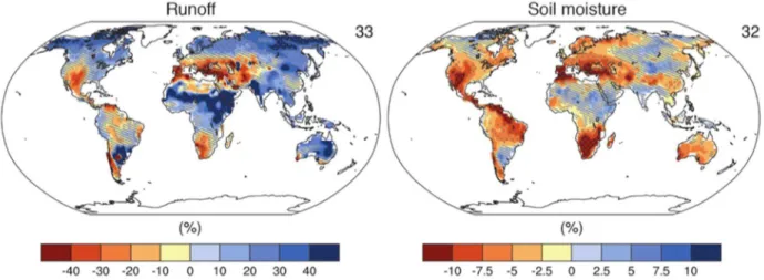
It has also been found that the annual runoff increases in higher latitude regions (Finland, China and coterminous US) while a decreasing patterns can be found in lower latitude regions such as

(21)

parts of West Africa, southern Latin America and southern Europe (IPCC, 2013; see Figure 4). Labat et al. (2004) observed a direct relationship between global annual temperature rise and global runoffs for the last century. It is estimated that global runoff increases by 4% per 1ºC increase in global temperature. Future projections of runoff and soil moisture at the global scale are shown in Figure 4. These projections are dependent on precipitation, which is itself subject to substantial uncertainties. However, it is important to know what climate models are projecting for the future. The left panel in Figure 4 predicts changes in surface runoff, with significant declining patterns in runoff throughout the southwestern US and southern Europe/northern Africa and parts of South America. This same trend is amplified in predictions of soil moisture, which is a primary control on plant growth.

Figure 4: Annual mean changes in runoff and soil moisture for 2081–2100 relative to 1986–2005 under the RCP8.5. The number of Coupled Model Inter-comparison Project Phase 5 (CMIP5) models to calculate the multi-model mean is indicated in the upper right corner of each panel. Hatching indicates regions where the multi-model mean change is less than one standard deviation of internal variability. Stippling indicates regions where the multi-model mean change is greater than two standard deviations of internal variability and where 90% of models agree on the sign of change. Source: IPCC (2013).

Based on the analysis of tide gauge data used in the AR5 (IPCC, 2013), the rate of global average sea level rise was found to be 1.5 to 1.9 mm/year, with a median value of 1.7 mm/year, for the 1901 to 2010 period and 2.8 to 3.6 mm/year, with a median value of 3.2 mm/year, for the 1993 to 2010 period. In addition, decreasing snow-cover (i.e. 11.7 % per decade for June in the Northern Hemisphere over the 1967 to 2012 period) and land ice extent (275 Gt/year over the 1993 to 2009 period) were found to be positively correlated with increasing surface temperatures (IPCC, 2013). Precipitation in tropical areas (30°S to 30°N) has increased during the 2000 to 2010 period compared to mid-1970s to mid-1990s. Also, in mid-latitude of the northern hemisphere (30° N to 60° N), a significant increasing precipitation trend was found over the 1901 to 2008 period, while in the southern hemisphere (30° S to 60° S), an abrupt declining trend was observed in precipitation during the 1979 to 2008 period (IPCC, 2013).

As summarized above, significant evidence of climate change exists at the global scale,

(22)

warming in Canadian Arctic has been almost double the rate of change for the rest of the world. Annual mean temperature for Canada has increased by 1.6°C for the 1948–2013 period, with increases of 1.3°C for southern Canada (i.e., south of the 60°N parallel) and 2.2°C for northern Canada (i.e., north of the 60°N parallel) (Bush et al., 2014; Environment and Climate Change Canada, 2016). Seasonally, winter and spring has seen the greatest warming. A warming climate will also lead to changes in precipitation characteristics, including the frequency and severity of precipitation extremes. In general, Canada has become wetter, as the total annual precipitation has increased by about 16% over the 1950 to 2010 period, but there are regional and seasonal differences across the country. Mekis and Vincent (2011) reported that in Canada, especially on the west coast, the total precipitation has increased in the fall and spring seasons, while it has decreased in the winter season during the 1950 to 2010 period. Winter precipitation has decreased because of decreases in winter snowfall due to warmer air temperatures. Many land regions, including Canada, have also observed increases in the number of heavy precipitation events (e.g. 95th percentile and larger values) (IPCC, 2013; Bush et al., 2014). The increases in daily precipitation extremes have been found to be greater than the increase in mean precipitation (IPCC, 2013). The increases in precipitation have been consistent with observed increases in atmospheric water vapour content over Canada and other parts of the world (IPCC, 2013; Vincent et al., 2007). On average, increases in annual precipitation could lead to reduced capacity of the soil to absorb moisture and possibility of increased flooding in case of heavy precipitation events.

The above discussed changes in historical climate and projections of future climate will have significant implications for river flows, urban runoffs, and storminess along the coasts. These changes will have significant implications for design flows and water levels which are

commonly used for generating floodplain maps. Consequently, it is natural to expect that the future design flows and water levels will be quite different from those derived from historical observations in many regions of Canada. Before presenting an inventory of methods for generating future design flows and water levels, a succinct but an informed description of climate models, emissions scenarios, climate downscaling, and future projections and associated uncertainties is provided below to provide the reader with a sufficient background on the subject matter of this report. Every effort has been made to keep the descriptions simple and not overly laborious for a common reader. Selection of global model outputs and appropriate downscaling methods is an integral part of the entire process of generating future flows and water levels.

2.2 Global Climate Models and Emissions Scenarios

The primary tools that are used to study anticipated climate change are the Global Climate Models (GCMs) and the transient climate change simulations produced when these models are integrated from the recent past to some time-point in the future with prescribed, time-evolving emissions scenarios for anthropogenic GHGs and aerosols (IPCC, 2007); emissions scenarios are

(23)

prescribed later in this section. These models numerically represent the climate system by encapsulating the current understanding of the climate system, the complex interactions between the atmosphere, ocean, land surface, snow and ice; the global ecosystem; and a variety of

chemical and biological processes (IPCC, 2013). GCMs produce global climate variables at grid cells that range from 100 to 300 km in horizontal resolution. Due to this coarse spatial resolution, GCMs are often unable to capture local features (such as undulating topography, local

waterbodies, sub-grid glaciers, etc.) and non-smooth climatic fields (such as precipitation originating from local convection activity). However, GCMs have been found to present

considerable skill in capturing large scale climatic features (IPCC, 2007, 2013). To study impacts of climate change at local and regional scales, downscaling methods are often employed for transferring coarse-scale climate information to local and regional scales. These methods are discussed below in Subsection 2.3.

To estimate future emissions and concentrations of GHGs in the atmosphere, IPCC has

developed many long-term emissions scenarios. For the Third Assessment Report and the AR4, IPCC discussed six families of scenarios: A1F1, A1T, A1B, A2, B1 and B2. These are

commonly known as Special Report on Emissions Scenarios (SRES) (Nakicenovic et al., 2000), which have now been superseded by new scenarios since the AR5. Mostly, A1B, A2, B1 and B2 have been used in climate change studies. A1B represents a rapid technological and demographic growth until mid-21st century after which global population decreases and a balanced emphasis on all energy sources continues. The A2 scenarios are of a more divided world with regionally oriented economic development that is more fragmented. B1 scenarios represent a rapid

demographic growth until mid-21st_{century, after which it decreases and the introduction of clean} and resource efficient technologies occurs. The B2 scenarios are of a world more divided, but more ecologically friendly. The B2 scenarios are characterized by local solutions to economic, social and environmental sustainability. More detailed information can be found in Nakicenovic et al. (2000).

For the AR5, IPCC developed a new set of long-term emissions scenarios, known as

Representative Concentration Pathways (RCPs), to estimate future emissions and concentrations of GHGs in the atmosphere (IPCC, 2013). RCPs were developed based on emissions of GHGs and they do not consider natural emissions such as volcanic eruptions. These scenarios describe how radiative forcing may influence future emissions scenarios and associated uncertainties. Based on an approximate level of total radiative forcing in the year 2100 compared to 1750, four RCPs (i.e. RCP2.6, RCP4.5, RCP6.0 and RCP8.5) have been mentioned in the AR5 (IPCC, 2013). These RCPs respectively correspond to 2.6 Wm-2, 4.5 Wm-2, 6.0 Wm-2 and 8.5 Wm-2 radiative forcings. IPCC refers to RCP2.6 as the mitigation scenario and RCP4.5 and RCP6.0 as the stabilization scenarios. RCP8.5 scenario corresponds to the maximum and unabated GHGs emissions and therefore, represents a sort of upper bound scenario.

(24)

2.3 Climate Downscaling

GCMs simulate present day climate and predict future climate, with forcings from GHGs

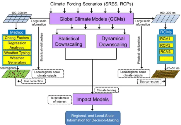
emissions scenarios. Since GCMs provide information on the large scale, specialized approaches and automated tools are required for transferring that large scale information from GCMs’ grids to local and regional scales in order to drive impact analysis models. The output from these models is used to assess impact of climate change on targeted assets (e.g. built infrastructure systems), various sectors of the society and environmental and ecosystem components. To make best use of the large scale GCM climate change simulations for impact analysis at local and regional scales, scientists have devised downscaling approaches. These approaches can be classified into two main categories: (i) dynamical downscaling and (ii) statistical downscaling. These approaches are schematically shown in Figure 5, along with selected techniques often used and recommended for generating local scale information. Further detail on these two categories of climate downscaling is provided below.

2.3.1 Dynamical Downscaling

Dynamical downscaling uses Regional Climate Models (RCMs) that like GCMs numerically describe various atmospheric processes at finer spatial resolutions, with typical grid cells of the order of 50 km x 50 km. Some climate modelling groups have now started running RCMs at even 5 to 10 km horizontal resolutions and the efforts are still on-going to further improve RCM resolutions. These models are applied over limited-area domains, with boundary conditions taken from global models (Caya and Laprise, 1999; Pal et al, 2007; Di Luca et al., 2012, 2013;

Scinocca et al., 2015).

Though physical representations of climate processes in RCMs are comparable to those in GCMs, typically RCMs are run without interactive ocean and sea-ice. Compared to GCMs, RCMs offer higher spatial resolution, allow for greater topographic complexity and finer-scale atmospheric dynamics to be simulated and hence provide more adequate tools for generating fine scale climate change information required for many impact and adaptation studies (Fesser and Barcikowska, 2012; Curry et al., 2016). Due to these advantages of RCMs, numerous studies have used RCM simulations for assessing future changes to various characteristics of

precipitation and temperature variables, including extreme events, in different parts of the world (e.g. Booij, 2002; Christensen and Christensen, 2003; Semmler and Jacob, 2004; Fowler et al., 2005; Ekström et al., 2005; Frei et al., 2006; Sushama et al., 2006a; Beniston et al., 2007; May, 2008; Nikulin et al., 2011; Poitras et al., 2011; Mladjic et al., 2011; Mailhot et al., 2012; Monette et al., 2012; Huziy et al., 2013; Jeong et al., 2014, 2015, 2016; and Jeong and Sushama, 2018, among many others).

RCMs are able to explicitly resolve regional waterbodies and land surface heterogeneities, thus allowing realistic feedback processes, which are important to reasonably simulate the climate system. Accounting for local waterbodies is essential for regions like Great Lakes area, as their

(25)

influence on regional climate can be considerable (Martynov et al., 2012; Huziy and Sushama, 2016a, 2016b). Huziy and Sushama (2016a, 2016b) demonstrated significant improvements to the timing and magnitude of spring peak flows and winter low flows when lake-river interactions were taken into account in the Canadian Regional Climate Model (CRCM). Similarly,

incorporating dynamic glaciers (Ruman and Sushama, 2016), dynamic vegetation (Garnaud et al., 2012, 2014), interactive permafrost (Sushama et al., 2006b), and localized processes (such as lake-effect-snow; Huziy et al., 2017) help produce more realistic current and future climate simulations. Another emerging benefit of RCMs is that they are quite useful in performing anthropogenic attribution related studies for targeted catastrophic weather and climate events. For example, to investigate if the anthropogenic influence has contributed or not to the 2013 Alberta flood, Teufel et al. (2016) conducted regional climate modelling experiments based on the CRCM. Similar investigations for the 2017 Montreal and Gatineau floods were conducted by Teufel et al. (2018) based on the CRCM simulations. Also, similar investigations for other localized weather and climate events of significant regional importance can be undertaken based on RCMs. The major drawback of the dynamical downscaling approach is high computational cost, dependence on boundary conditions from GCMs and difficulty of direct transferability of a working RCM from one region to another region.

Figure 5: A schematic diagram of climate downscaling to drive impact models for climate change studies at local and regional scales (adapted and modified from Khaliq, 2018). Abbreviations are described in the text.

(26)

Statistical downscaling (SD) methods use empirical relationships between large-scale GCM simulated climate variables (treated as predictors) and regional or local scale climate variables (treated as predictands). For example, GCM-derived values of specific humidity, sea level

pressure, geopotential heights and areal precipitation and temperature as predictors versus locally observed precipitation or temperature as a predictand at a given point of interest. Often three important assumptions are made when using this approach (Hewitson and Crane, 1996; Wilby and Wigley, 1997):

 Predictor variables are realistically modelled by GCMs;

 The empirical relationship between predictors and predictand is valid for current and future climate conditions, irrespective of stationary or evolving climatic conditions; and  The predictors fully represent the climate change signal.

Though single site downscaling is quite common, techniques have also been developed to consider multiple climatic variables simultaneously at multiple sites in order to preserve some physical consistency across variables and across the region being studied (e.g. Zhang and Georgakakos, 2012; Jeong et al., 2012; Khalili et al., 2013; Asong et al., 2016; Khalili and Nguyen, 2018). Sources of model errors and uncertainties in statistical downscaling depend on the choice of method, including the choice of predictors, estimation of empirical relationships between predictors and predictands from limited data sets, and also on the quality of data used to estimate predictors (Frost et al., 2011; Wilby and Dawson, 2012). The relationships inferred from historical data may not remain valid under a changing climate in the future. A good performance of a statistical downscaling method as assessed against observations does not guarantee credible future climate projections. These relationships may also break down if far out in the future climate change happens in a dramatic manner and new feedback emerges that climate science is not expecting. The statistical downscaling approach is not based on physical laws, ignores climate feedbacks and often underestimates extreme values (such as precipitation extremes). Despite these drawbacks, statistical downscaling is more adaptable and flexible and is popular also because of low computational cost and ease of use. There are numerous statistical downscaling methods, and the findings are difficult to generalize (IPCC, 2013). However, SD methods can be classified broadly into three categories (Wilby and Wigley, 1997): (i) weather typing methods; (ii) regression- or transfer function-based methods, and (iii) stochastic weather generators (WGs). Another class of SD methods that downscale as well as bias-correct climate model outputs is described separately below in Section 2.4. There are a number of studies wherein these methods have been used. Only selected studies are referred to in the descriptions of these methods, provided below. Though generally SD approaches have been used for

downscaling global model outputs, they are equally applicable to further downscale outputs from regional climate models (Teutschbein and Seibert, 2012).

Weather Typing: Weather typing downscaling approaches are based on specific weather classification schemes and exploit relationships between local climate variables and

(27)

synoptic-scale atmospheric circulation patterns. For developing such relationships, approaches like principal component analysis (PCA) (e.g. Wetterhall et al., 2005), fuzzy rules (Bardossy et al., 1995), canonical correlation analysis (CCA) (e.g. Gyalistras et al., 1994), and analogue

procedures (Martin et al., 1997) have been used. Some investigators have also used pattern recognition approaches based on correlation analyses (e.g. Wilby and Wigley, 1997). Though this approach is appealing because it is founded on sensible physical linkages between climate on the large-scale and weather at the local-scale, it is known to have difficulty in simulating extreme events (Wilby, 1997). The major drawback of weather typing approaches is that they use the same stationary relationships, between local climate variables and synoptic-scale atmospheric circulation patterns, throughout from historical to future climates. Furthermore, the additional effort of adopting a suitable weather classification scheme makes them further less attractive. Regression- or Transfer Function-based Methods: These methods rely on a statistical

relationship between GCM outputs (as large-scale predictors) and local-scale climate variables (as predictands). For this purpose, multivariate linear or nonlinear regressions (e.g. Vrac et al., 2007; Chen et al., 2014), non-parametric regression (e.g. Sharma and O’Neill, 2002; Kannan and Ghosh, 2013) and machine learning approaches (e.g. Tripathi et al., 2006; Ghosh, 2010) have been used to establish predictor-predictand relationships. These approaches are widely used for statistical downscaling purposes. For a given problem, it is possible to experiment with a number of large-scale predictors, but a smaller set of surface/pressure variables has often been used (e.g. specific humidity, sea level pressure, geopotential height, and U and V components of wind velocity). The predictor variables are desired to be uncorrelated in order to satisfy certain theoretical assumptions and to avoid overfitting. Ignoring these aspects may result in spurious relationships leading to false hypotheses. It has been found that nonparametric statistical methods like the K-nearest neighbors (Brandsma and Buishand, 1998; Sharif and Burn, 2006; Eum and Simonovic, 2012; King et al., 2014) and Kernel density estimators (Kannan and Ghosh, 2013) can be considered as plausible alternate approaches for statistical downscaling. Although non-parametric methods can capture the spatial dependence of observed climatic variables, they were found to be unable to simulate extreme observations, specifically precipitation extremes. Markov chain based SD methods (e.g. Hughes and Guttorp, 1994; Mehrotra and Sharma, 2007) were found to perform satisfactorily in capturing spatial variability of precipitation, but were found to have difficulties in reproducing observed variability. Coulibaly et al. (2005) developed a statistical downscaling method based on a time-lagged feed-forward neural network (TLFN) method. A major assumption of the method was that the local climate variables (e.g.

precipitation and temperature) depend on both present and past large-scale states of the

atmosphere. The performance of TLFN method in downscaling precipitation and temperature has been found better than many other methods (e.g. the downscaling method proposed by Wilby et al., 2002). However, some deficiencies were also found, e.g. overestimated values of wet-spell length. This was the case at the time TLFN method was proposed. A number of improved

(28)

additional approaches that perform much better than the TLFN method have been introduced afterwards.

Weather Generators: Weather generators (WGs) are statistical tools that stochastically simulate random sequences of climate variables. When fitted to observed sequences of climate variables, they tend to preserve their statistical properties (e.g. Wilks and Wilby, 1999; King et al., 2014). Mehrotra and Sharma (2005) developed a K-nearest-neighbor based nonparametric

nonhomogeneous hidden Markov model (NHMM) for downscaling multisite rainfall sequences over a network of 30 gauging stations near Sydney, Australia. The NHMM generates rainfall sequences based on average rainfall occurrence over the previous day, conditional to a continuous weather state. Following insights from this study, King et al. (2014) developed another non-parametric multisite WG based on the K-nearest-neighbor approach. This WG also considers block resampling and perturbation mechanisms and was used for downscaling daily temperature and precipitation data in the Upper Thames River basin, Ontario. In addition to simulating historical climate, this WG is also able to simulate extreme values beyond the range of historical observations when applied in a downscaling setting (King et al., 2014). Srivastava and Simonovic (2014) developed a non-parametric multisite, multivariate maximum entropy based WG for simulating daily precipitation and minimum and maximum temperatures. This WG can capture temporal and spatial dependencies of historical temperature and precipitation variables along with other basic statistical properties (such as mean and standard deviation) in downscaled climatic variables. The authors have found that this approach is computationally quite efficient.

Generalized linear model (GLM) based WGs benefit from the strengths of both regression- and WG-based techniques. Using GLMs, Chandler and Wheater (2002) found that such WGs give accurate simulations of mean rainfall at the seasonal scale. Inspired by the flexibility of the GLM framework, Chun et al. (2013) compared Long Ashton Research Station weather generator (LARS-WG) and GLM approach for single-site downscaling of daily precipitation at four selected locations in western Canada. The GLM based approach out-performed the LARS-WG in terms of simulating various characteristics of extreme events, as well as inter-annual

variability. The GLM based approach allows for inclusion of external covariates unlike LARS-WG. A particular strength of GLM based approach is the use of interaction terms to deal with situations in which some covariates modulate the effects of others. It is important to note that LARS-WG has been used extensively in downscaling studies across the world. One possible reason could be that the LARS-WG software is readily available and is easy to implement. Albeit with some drawbacks, the GLM based approach seems to be quite suitable for SD of GCM outputs.

(29)

Bias correction pertains to the process of adjusting climate model outputs to reduce their discrepancies from observations for a given reference historical period. Sometimes these discrepancies could be due to systematic errors in climate models originating from deficiencies in numerical parametrizations. Once a suitable bias correction method is identified based on a given reference historical period, the same is assumed to be valid for future projections. Bias correction methods were originally designed to downscale GCM outputs and therefore they are also categorized as statistical downscaling methods. For example, the quantile mapping or the probability mapping procedure which directly maps quantiles of GCM outputs (e.g. temperature and precipitation) onto the quantiles of observations at a given point in space, lying within the domain of the GCM grid cell, downscales as well as bias corrects GCM outputs. Following Edwards and McKee (1997), the quantile mapping is an equiprobability transformation (Panofsky and Brier, 1958) which states that the essential features of transforming one variate from one distribution to another prescribed distribution such that the probability of being less than a given value of the variate shall be the same as the probability of being less than the corresponding value of the transformed variate.

Several bias correction methods have been developed to bias correct climate model outputs and their performance varies from one application to another and also from one climate variable to another (e.g. Johnson and Sharma, 2011). These methods can be classified in various ways. According to Teutschbein and Seibert (2012), bias correction of climate model outputs considerably improves hydrological simulations, but the major drawback is that nearly all methods assume stationary model structures (i.e. the algorithm along with its parameters) and that may not be valid under changing climate conditions (Maraun, 2012). Most bias correction methods can also be used with RCM outputs. In that case they can also be classified as post-processors which are used to bias correct or further downscale RCM outputs. In Canada, Werner (2011) has used Bias Corrected Spatial Disaggregation (BCSD) algorithm, based on the work of Wood et al. (2004), Salathé (2005) and Slathé et al. (2007), to downscale and bias correct GCM outputs at the grid resolution of the VIC (Variable Infiltration Capacity) model (Liang et al., 1994) for hydrological modelling purposes in British Columbia. This method is further evaluated in Bürger et al. (2012). A few variants of the BCSD algorithm, along with bias correction

constructed analogues (BCCA), double BCCA, BCCA with quantile mapping reordering, the climate imprint delta method (CI), and bias corrected CI methods have been reported and

evaluated in Werner and Cannon (2016) to downscale precipitation and temperature outputs from CMIP5 simulations to drive the VIC model over the Peace River basin in British Columbia. Despite many advantages of bias correction methods, climate modelling community has raised a number of concerns, e.g.

 A proper physical foundation for these methods does not exist (Teutschbein and Seibert, 2012). The physical causes of climate model biases are totally ignored when developing

(30)

bias correction methods and bias corrected model outputs may become physically inconsistent;

 Conservation of mass and momentum principles and feedback mechanisms on which the climate models are based are not preserved in these methods (Ehret et al., 2012);

 The stationarity of the parameters and structure of the bias correction method from the reference historical period to the future time period is difficult to justify (as also mentioned in the above discussion);

 The likelihood of altering the true climate change signal cannot be ruled out (Dosio et al., 2012);

 As multiple methods exist, the choice of bias correction method introduces an additional source of uncertainty (Teutschbein and Seibert, 2012) in the results of impact models; and

 Given other major sources of uncertainties, the added value of bias correction may become insignificant.

In spite of the above mentioned limitations of the bias correction methods they are commonly used in climate change impact analysis studies, particularly in hydrological applications.

Perhaps, the best solution would be to improve the physics and resolution of climate models and that may be forthcoming, after several years into the future.

2.5 Climate Projections and Uncertainties

As mentioned before, information about climate variables from GCMs is available at large spatial grids that could range from 100 to 300 km in horizontal resolution, depending upon the GCM. To generate local and regional scale information of selected climate variables (e.g. precipitation and temperature), climate downscaling is the preferred approach. Statistical downscaling uses a range of statistical approaches, while dynamical downscaling uses RCMs driven by boundary conditions taken from GCMs to generate fine resolution gridded

information. Following this linked chain of modelling and downscaling methods, the downscaled information is subject to considerable amount of uncertainty, originating from several sources, e.g.

 Inter-GCM variability due to different model structures,

 Quality of emissions scenarios and inter-scenario variability due to different types of emissions scenarios (different SRES families and the RCPs),

 Intra-model variability due to different parametrizations, and

 The choice of downscaling methods – both statistical and dynamical downscaling methods introduce many other sources of uncertainties, apart from those related to GCMs.

(31)

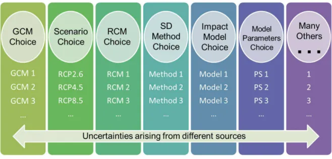
The AR5 of the IPCC (IPCC, 2013) demonstrate that scenario related uncertainties dominate by the end of the 21st_{century, while some other investigators (e.g. Prudhomme and Davies, 2009a,} 2009b) have found that GCM related uncertainties dominate all other uncertainties if a single downscaling method is used. For all practical applications, it is important to quantify various sources of uncertainties in climate variables as these uncertainties propagate further in the outputs of impact models, which are driven by these variables. For example, often hydrological models are used to project future flows from a given watershed under climate change conditions. These models are forced with projected meteorological variables (e.g. precipitation, temperature, evapotranspiration, etc.). The projected streamflow from these models will carry uncertainties present in the downscaled GCM outputs. For certain applications, some investigators use multiple hydrological models, having different structures and different process representations, and that could introduce additional sources of uncertainties (e.g. Dibike and Coulibaly, 2005; Najafi et al., 2011; Schnorbus et al., 2011; Surfleet and Tullos, 2013). Given various sources of uncertainties (see Figure 6) and to derive meaningful results from the output of impact models, it is important to quantify these uncertainties in a reasonable and objective manner. One possibility is to use multiple GCMs, multiple scenarios, multiple downscaling techniques, multiple bias-correction methods, and multiple impact models. This seems to be overkill from the viewpoint of the significant amount of effort involved, but appears to be a scientifically defensible approach.

Figure 6: A conceptual depiction of different sources of uncertainties associated with climate model projections. The abbreviations used in the diagram are: GCM–Global Climate Model; RCP–Representative Concentration Pathway; RCM– Regional Climate Model; SD–Statistical Downscaling; PS–Parameter Set.

(32)

3 An Inventory of Methods for Estimating Design Flows

and Water Levels in Riverine and Urban Environments

3.1 General

Floodplain maps provide information on potential flooding situations and are commonly used for land use planning purposes and to regulate future land development activities. In some

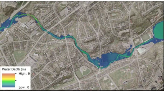
jurisdictions, floodplain maps are highly detailed and can provide flood risk information even at the household level. In some countries, an additional objective of floodplain maps is to support information on flood loads and intensities for codes and standards development. From an economic viewpoint, an important objective is to minimize flood damages by providing reliable information on flood risks through floodplain maps. Several different types of floodplain maps have been developed in response to this diverse set of considerations and applications. For example: inundation maps–that only show horizontal flooding extents; flood hazard maps–that show hazard zones depending upon the degree of hazard based on either depth or velocity criterion; flood risk maps–that show detailed spatial information on flood depth and velocity and exposure/vulnerability of different assets. A few selected examples of floodplain maps are shown in Figure 7 and Figure 8. There is no standardized naming convention for floodplain maps so inferences from maps can mean different things in different parts of the world.

Figure 7: (a) Flood hazard map for Badger, NL (source: Water Resources Management Division, Department of Municipal Affairs and Environment, Government of Newfoundland and Labrador) showing flood hazard zones corresponding to 20-year and 100-year flood flow inundation levels. (b) Flood hazard map of Calgary, AB (source: Alberta Environment and Parks, Government of Alberta) showing flood hazard zones corresponding to floodway (where velocity is ≥ 1 m/s and depth is ≥ 1 m) and flood fringe (where velocity is < 1 m/s and depth is < 1m).

Reliable information on design flows and water levels is an important input that is essential for developing floodplain maps. Estimation of design flows and water levels is closely tied with climatic variables (e.g. precipitation and temperature), which are projected to change due to