Analyzing pulse from head motions in video

Analyzing Pulse From Head Motions in Video

by

Guha Balakrishnan

Submitted to the Department of Electrical Engineering and Computer

Science

in partial fulfillment of the requirements for the degree of

Master of Science in Computer Science and Engineering

at the

MASSACHUSETTS INSTITUTE OF TECHNOLOGY

February 2014

ARCNE$

APR

10

201

ui BARIES

@

Massachusetts Institute of Technology 2014. All rights reserved.

Author.

.

_{epartment of El'ectrical}

.en

.o

. ...

Engineering and Computer Science

October 1, 2013

Certified by

.

...

Professor, Electrical Engin

g and

John Guttag

Computer Science

Thesis Supervisor

C ertified by ...

...

Fredo Durand

Professor, Electrical Engineering and Computer Science

Thesis Supervisor

Accepted by ...

0

Leslie A. Kolodziejski

Analyzing Pulse From Head Motions in Video

by

Guha Balakrishnan

Submitted to the Department of Electrical Engineering and Computer Science on October 1, 2013, in partial fulfillment of the

requirements for the degree of

Master of Science in Computer Science and Engineering

Abstract

We extract heart rate and beat lengths from videos by measuring subtle head oscil-lations that accompany the cardiac cycle. Our method tracks features on the head, temporally filters their trajectories and performs principal component analysis (PCA) to decompose the trajectories into a set of ID component motions. It then chooses the component that is most periodic as the pulse signal. Finally, we identify peaks of the chosen signal, which correspond to heartbeats. When evaluated on 18 subjects our

approach reported heart rates nearly identical to an electrocardiogram (ECG) device for all subjects and obtained similar beat length distributions for 17. In addition we obtained pulse rate from videos of the back of the head and of sleeping newborns.

Initial findings also show that our method can measure heart rate from body parts other than the head and can measure respiration rate by selecting a different frequency band. Finally, we present visualization techniques such as motion magnification for subjective analysis of body motions.

Thesis Supervisor: John Guttag

Title: Professor, Electrical Engineering and Computer Science

Thesis Supervisor: Fredo Durand

Acknowledgments

I first thank my advisors John Guttag and Fredo Durand for making this research a

fun endeavor and bringing their knowledge, guidance and optimism to the work.

I thank the members of the Data Driven Medical Group: Joel, Anima, Garthee,

Jenna, Jen, Amy and Yun for their advice and comments over the past couple of years. They also patiently sat through my video recording sessions, which were critical for my experiments. Thanks to Collin Stultz who helped keep our work on track from the medical perspective. I also appreciate the feedback from Bill Freeman, Tiam Jaroensri, Michael Rubinstein and Neal Wadhwa. Their related research in the computer vision/medical space was a motivating force for me.

Finally I am grateful to my family, who have always taken an interest in my academic progress. They made it very easy for me to concentrate on my graduate work and supported me in many ways.

Contents

2.1 The Cardiac Cycle and Ballistocardiac Forces . . . . 2.1.1 A ortic Force . . . . 2.1.2 C arotid Force . . . .

2.1.3 Heart Rate and Heart Rate Variability . . . . 2.2 Optical Flow and the Lucas-Kanade Algorithm . . . . 2.3 Color-Based Pulse Detection from Video . . . .

3 Method

3.1 Region Selection . . . .

3.2 Feature Point Selection

3.3 Feature Point Tracking 3.4 Temporal Filtering 3.5 PCA Decomposition 3.6 Signal Selection . . . . 3.7 Peak Detection . . . . 4 Experiments 15 16 17 18 19 19 20 21 22 23 25 27 29 29 30 30 30 33 35 37 . . . . . . . .

4.1 V isible Face . . . . 37

4.1.1 Motion Amplitude ... ... 39

4.1.2 Noise Analysis . . . . 41

4.1.3 Comparison to Color-Based Detection . . . . 47

4.2 Other Views of the Head . . . . 48

4.3 Sleeping Newborns . . . . 48

4.4 D iscussion . . . . 49

5 Other Applications of Our Method 51 5.1 Pulse From Other Body Parts . . . . 51

5.2 R espiration . . . . 52

6 Visualization Techniques 55 6.1 Single Images . . . . 55

6.1.1 Eigenvector Plot . . . . 56

6.1.2 Frequency Trajectory Plots . . . . 56

6.2 Video Motion Amplification . . . . 57

6.3 Basic Amplification . . . . 58

6.4 Typical Beats . . . . 58

6.4.1 Input . . . . 59

6.4.2 Algorithm . . . . 60

7 Summary & Conclusion 63

List of Figures

2-1 Blood flows from the heart to the head via the carotid arteries on either side of the head [14]. . . . . 19

2-2 An old model of a ballistocardiogram where a subject lies on a low-friction platform. The displacement and/or acceleration of the body is measured to infer cardiac output. Image courtesy of Nihon Kohden. . 21

2-3 Example of typical ECG signal. Differences between R peaks in suc-cessive beats of an ECG can be used to calculate heart rate variability or H R V . . . . 22 2-4 Overview of color-based pulse detection method (image taken from

[18]). A face is found from the first video frame to construct a region of

interest (ROI). The red, green and blue channels are spatially averaged in the ROI in each frame to form three signals. ICA is applied on these signals to obtain three independent source signals. The most periodic source signal is chosen for analysis. . . . . 24

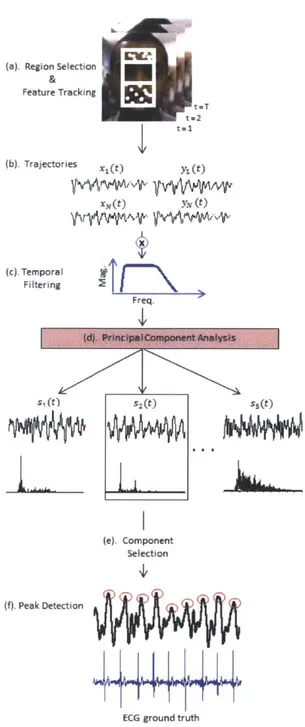
3-1 Overview of our pulse estimation approach. (a) A region is selected within the head and feature points are tracked for all frames of the video. (b) The horizontal and vertical components are extracted from each feature point trajectory. (c) Each component is then temporally filtered to remove extraneous frequencies. (d) PCA decomposes the trajectories into a set of source signals S1, S2, S3, S4, S5. (e) The

compo-nent that has clearest main frequency is selected. (f). Peak detection identifies the beats of the signal. . . . . 28

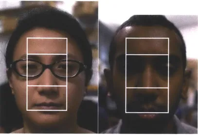
3-2 The region of interest for subjects 1 and 2. The region encompasses the m iddle of the face. . . . . 29

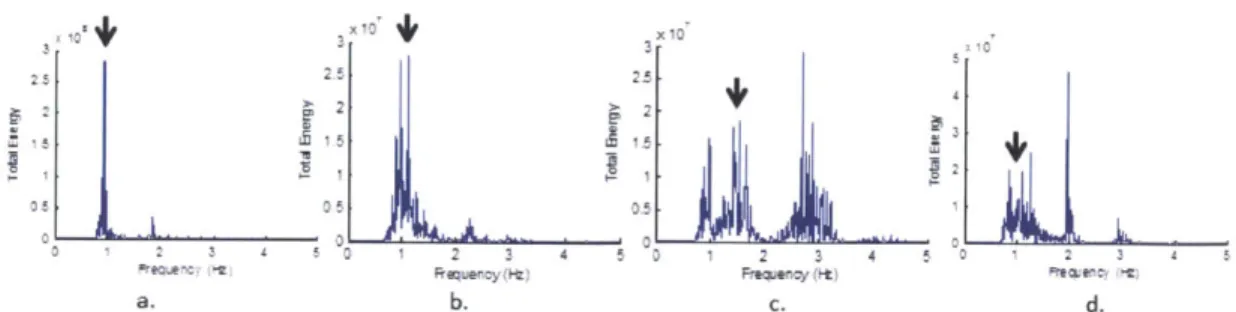
3-3 Examples of the combined energy spectra of feature points for 4 dif-ferent subjects. (a) is an example where the pulse frequency is the only dominant frequency. (b) is an example where there is another fre-quency with nearly as much energy as pulse. (c) is an example where the harmonic of the pulse frequency has more energy than the pulse frequency. (d) is an example where the energy at the pulse frequency is smaller than several other peaks in the spectrum. We were able to get accurate pulse signals for all subjects using our method which separates the combined motion of the feature points into submotions

using P C A . . . . . 31

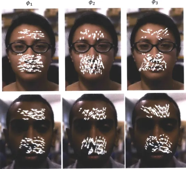
3-4 Examples of the first three eigenvectors for two subjects. Each white arrow on a face represents the magnitude and direction of a feature point's contribution to that eigenvector. The eigenvector decomposi-tion is unique to each video. . . . . 32

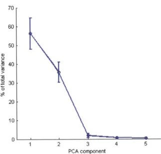
3-5 Percentage of total variance explained by the first five PCA compo-nents, averaged over all subjects in our experiments. Bars are stan-dard deviations. The first component explains most of the variance for all subjects. However, the first component may not produce the best signal for analysis. . . . . 34

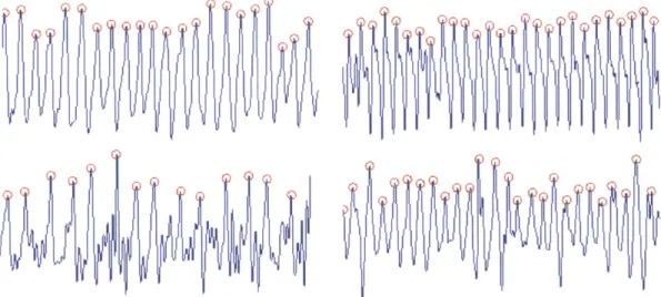
3-6 Examples of motion signals outputted by our method. Red circles are peaks. ... ... 35

4-1 Reference frames from videos of all 18 subjects. Subjects varied in skin color, gender and age. . . . . 38

4-2 Beat distributions of the ECG and our motion method for subjects. (a) We were able to accurately capture a wide range of distribution shapes, such as for subjects 4, 17, 1 and 6. (b) We were not able to produce an accurate distribution for subject 5. . . . . 40

4-3 Frames from videos of subject 1 with varying levels of additive gaussian noise. The top row shows frames before filtering. The bottom row shows frames after bilateral filtering. Noise ranged from a standard deviation of 5 to 500 pixels. Bilateral filtering smooths images while retaining edges. . . . . 41

4-4 Plots presenting results after adding varying levels of Gaussian noise

to our videos. (a) shows omaxnoise, the standard deviation of the first

noise level at which our method gave an incorrect average pulse rate.

(b) shows the number of similar distributions reported by the KS test

as noise is added to the videos. . . . . 43

4-5 Plots of 0maxnoise vs. 0 and -y our two metrics measuring head motion

strength. Both variables are significantly correlated with 7maxnoise. . . 44

4-6 Analysis of K, our metric measuring feature point quality. . . . . 45

4-7 The average 0maxnoise of all subjects vs. the number of feature points

selected. 1500 points is the number of feature points used in the original results (see Fig. ??). We selected points in three ways: randomly around the region of interest, by the highest K and by the lowest K. The random results were repeated 10 times and averaged. Random selection and the high , selection peformed similarly while low / yielded the worst results. Adding more feature points increased 0maxnoise for all sampling methods but helped the low K method the most. . . . . 46

4-8 Comparison of our method to color-based detection. 7maxnoise is the maximum noise standard deviations where either color and motion give reliable results. Our method worked longer (under the blue dotted line) for 9 of the 18 subjects while color worked longer for 8 subjects. The color method failed to give a correct result for subject 7 before the

addition of noise. . . . . 47

4-9 Reference frames from two videos of the back of the head and one of a face covered with a mask. . . . . 48

4-10 Results from videos of sleeping newborns. Our method produces pulse rates matching the actual bedside monitors. . . . . 49

5-1 Pulse signals from the chest and carotid artery. . . . . 52 5-2 Respiration signals from 2 subjects (a,b) and a neonatal infant (c).

The rates for the two adult subjects were quite low, likely because they were told to sit still as possible for the videos. The rate for the infant is near a normal adult's pulse rate, which is typical for newborns. 53

6-1 Frequency trajectory plots. Red trajectories are points moving clock-wise and white are counterclockclock-wise. (a) is at the respiration frequency magnified 100 times. The ellipses from the left and right chest point away from each other since the chest expands and contracts when breathing. (b) is a plot at the pulse frequency magnified 1000 times. The head moves more than the chest in this case. . . . . 57 6-2 Example of applying a Delaunay triangulation to feature points on

subject 5's face. Red stars denote feature points and the blue lines show the triangulation between the points. . . . . 59 6-3 A comparison of a sequence of frames before and after applying motion

magnification. The head motion is much more visible after magnification. 59 6-4 The typical x and y feature point trajectory for each subject. . . . . . 61

List of Tables

4.1 Results when comparing the beat length distributions of the ECG and our method. Presented are the means (ip) and standard deviations (-) of the distributions along with p-value of the Kolmogorov-Smirnov test measuring distribution similarity. 17 of the 18 pairs of distributions were not found to be significantly different (p >= 0.05) . . . . 39

4.2 Mean (std. dev.) RMS amplitudes in pixels for the x and y feature point trajectories for all subjects. Values are shown after filtering to within 0.05 Hz of the pulse frequency (RMS Pulse) and without filtering

Chapter 1

Introduction

Heart rate is a critical vital sign for medical diagnosis. There is growing interest in extracting it without contact, particularly for populations such as premature neonates and the elderly for whom the skin is fragile and damageable by traditional sensors. Furthermore, as the population ages, continuous or at least frequent monitoring out-side of clinical environments can provide doctors with not just timely samples but also long-term trends and statistical analyses. Acceptance of such monitoring depends in part on the monitors being non-invasive and non-obtrusive.

In this thesis, we exploit subtle head oscillations that accompany the cardiac cycle to extract information about cardiac activity from video recordings. In addition to providing an unobtrusive way of measuring heart rate, the method can be used to extract other clinically useful information about cardiac activity, such as the subtle changes in the length of heartbeats that are associated with the health of the auto-nomic nervous system. Our method works with typical video recordings and is not restricted to any particular view of the head.

The cyclical movement of blood from the heart to the head via the abdominal aorta and the carotid arteries causes the head to move in a periodic motion. Our algorithm detects pulse from this movement. Our basic approach is to track feature points on a person's head, filter their positions by a temporal frequency band of interest, and use principal component analysis (PCA) to find a periodic signal caused

spectrum and obtain precise beat locations with a simple peak detection algorithm.

1.1

Related Work

Our method is an alternative to the extraction of pulse rate from video via analysis of the subtle color changes in the skin caused by blood circulation [18, 26]. These methods average pixel values for all channels in the facial region and temporally filter the signals to an appropriate band. They then either use these signals directly for analysis [26] or perform ICA to extract a single pulse wave [18]. They find the frequency of maximal power in the frequency spectrum to provide a pulse estimate. Philips produced a commercial app that detects pulse from color changes in real-time

[17]. These color-based detection schemes require that facial skin be exposed to the

camera. In contrast our approach is not restricted to a particular view of the head, and is effective even when skin is not visible.

There have also been studies on non-invasive pulse estimation using modalities other than video such as thermal imagery [6], photoplethysmography (measurement of the variations in transmitted or reflected light in the skin) [29] and laser and microwave Doppler [25, 7]. Noncontact assessment of heart rate variability (HRV), an index of cardiac autonomic activity, presents a greater challenge and few attempts have been made [21, 13, 15]. A common drawback of these non-invasive systems is that they are expensive and require specialized hardware.

The analysis of body motion in videos has been used in different medical contexts, such as the measurement of respiration rate from chest movement [23, 17], or the monitoring of sleep apnea by recognizing abnormal respiration patterns [28]. Motion studies for diseases include identification of gait patterns of patients with Parkinson's disease [4], detection of seizures for patients with epilepsy [16] and early prediction of cerebral palsy [1]. The movements involved in these approaches are larger in amplitude than the involuntary head movements due to pulse.

Our work is inspired by the amplification of imperceptible motions in video [30, 12]. But whereas these methods make small motions visible, we want to extract

quantitative information about heartbeats.

The idea of exploiting Newton's Third Law to measure cardiac activity dates back to at least the 1930's, when the ballistocardiogram (BCG) was invented [20]. The subject was placed on a low-friction platform, and the displacement of the platform was used to measure cardiac output. The BCG was never widely used in clinical settings. Other clinical methods using a pneumatic chair and strain-sensing foot scale have also been successful under laboratory conditions[11, 10]. Ballistocardiographic head movement of the sort studied here has generally gained less attention. Such movement has been reported during studies of vestibular activity and as an unwanted artifact during MRI studies [2]. Recently, He et al. [8] proposed exploiting head motion measured by accelerometers for heart rate monitoring as a proxy for traditional BCG.

1.2

Contributions

This thesis makes the following contributions:

1. Development of a method for extracting pulse rate and heartbeat variability

from videos by analyzing ballistocardiac motions of the head. Our method tracks feature points on the head, filters their trajectories to a frequency band of interest, and uses PCA to decompose the trajectories into 1-D signals. The most periodic 1-D signal is then chosen to calculate pulse rate and find beat intervals. Our method is not restricted to any view of the face, and can even work when the face is occluded.

2. Validation of our method on video recordings

(a) Our system returned pulse rates nearly identical to an electrocardiogram

(ECG) device for 18 subjects.

(b) We are the first to evaluate beat-length distributions from video as a way

to evaluate variability. We captured very similar beat length distributions to the ECG for our subjects.

(c) We extracted pulse rate from videos of the back of the head and when a subject was wearing a mask.

(d) We extracted pulse rate for several videos of sleeping infants.

3. Noise analysis of our method and a comparison to a color-based pulse detection

scheme [18].

4. Results showing that our method can also be used to measure respiration rate and extract pulse from movements in the chest and carotid artery. While our techniques were developed for measuring pulse from head motions, we tried to keep our technique general enough to not be limited to the head alone.

5. Presentation of visualization techniques such as frequency trajectory plots and

motion magnification for more subjective evaluation of body motions. These methods are useful for exploratory analysis of motions in video.

1.3

Thesis Organization

The rest of this thesis is organized as follows. Chapter 2 provides background of relevant physiology and computer vision techniques. Chapter 3 presents our method. In Chapter 4 we evaluate our method on video recordings. In Chapter 5 we present initial results showing how our method can be used for other applications. In Chap-ter 6 we present visualization techniques for subjective evaluation of body motions.

Chapter 2

Background

This section provides a brief background on several key topics related to our study. First we present the main elements of the cardiac cycle and the ballistocardiac forces that cause body and head motions. We then discuss the clinical significance of heart beat variability. We then give a simple overview of feature tracking, an important element of our pulse detection system. Finally we summarize a recent method on pulse extraction from changes in skin color to which we compare our work in our experimental evaluation.

2.1

The Cardiac Cycle and Ballistocardiac Forces

Aorta --Right Atrium Right Ventricle Left Atrium Left Ventricle ... Carotid Artery

Figure 2-1: Blood flows from the heart to the head via the carotid arteries on either side of the head [14].

The heart is is a hollow muscle that pumps blood throughout the body by re-peated, cyclical contractions. It is composed of four chambers: the left/right ventricle and the left/right atrium (Fig. 2-1). During the phase of the cardiac cycle known as

diastole, the ventricles relax and allow blood to flow into them from the atria. In

the next phase known as systole, the ventricles contract and pump blood to the pul-monary artery and aorta. The aorta in turn transports blood to the rest of the body. The head and neck receive blood from the aorta via the common carotid arteries, which further divide into the internal and external carotid arteries in the neck.

We are not certain how much of head motion we detect is attributable to the large acceleration of blood in the aorta compared to the localized acceleration of blood in the carotid arteries moving into the head. He et al. [8] measured ballistocardiac head motions with an accelerometer-based device to be on the order of 10 mG(0.098 M), but it is unclear what fraction of this movement is attributed to aortic and carotid blood flow forces. To understand this better, we will present derivations of the magnitude of each of these forces in Sections 2.1.1 and 2.1.2. The calculations are simplified, ignoring many details about fluid dynamics and physiology. From a biomechanical standpoint, the head-neck system and the trunk can be considered as a sequence of stacked inverted pendulums. This structure allows the head unconstrained movement in most axes, making calculations of the system's motion complicated.

2.1.1

Aortic Force

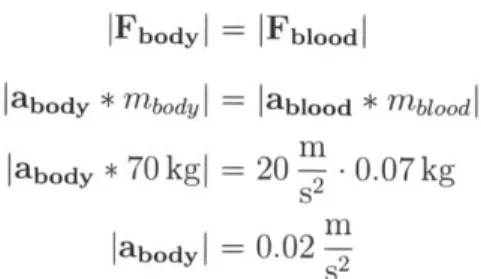
During systole a healthy adult aorta is capable of impelling a volume of 70 - 80 ml

(0.07 - 0.08 kg) of blood at considerable speed (1 1) and acceleration (20 m) [19].

An average adult male weighs 70 kg. Using Newton's 2,d and 3rd laws we derive the

IFbodyI = IFblood I

Iabody

m

labodyl =

0.02

Thus the approximate acceleration of the body due to the aortic forces is 0.02!! Ballistocardiography produces a graphical representation of body movement due to this force for a subject lying down on a low-friction platform (Fig. 2-2).

Figure 2-2: An old model of a ballistocardiogram where friction platform. The displacement and/or acceleration of infer cardiac output. Image courtesy of Nihon Kohden.

a subject lies on a low-the body is measured to

2.1.2

Carotid Force

In addition to aortic blood acceleration, there is the smaller force resulting from blood flowing through the carotid arteries into the head. Although there are studies measuring blood flow, velocity and acceleration of blood in the carotid, we have not found similar experimental measurements on the force imparted by carotid blood flow

on the head. According to one study, blood velocity in the common carotid increases from approximately 0.02 m to 0.11 !1 in 0.1 s, or an acceleration of 0.9 m [9]. The blood mass transported in this period is roughly 13 ml or 0.013 kg. Assuming both carotid arteries are identical and that the head is 5 kg, we use a similar derivation to the one used in Section 2.1.1 to find that the head should accelerate roughly 0.005 M

assuming independence from the rest of the body.

2.1.3

Heart Rate and Heart Rate Variability

Pulse rate captures the average number of cardiac cycles over a period of time (e.g.,

30 seconds). It is useful primarily for detecting acute problems. There is a growing

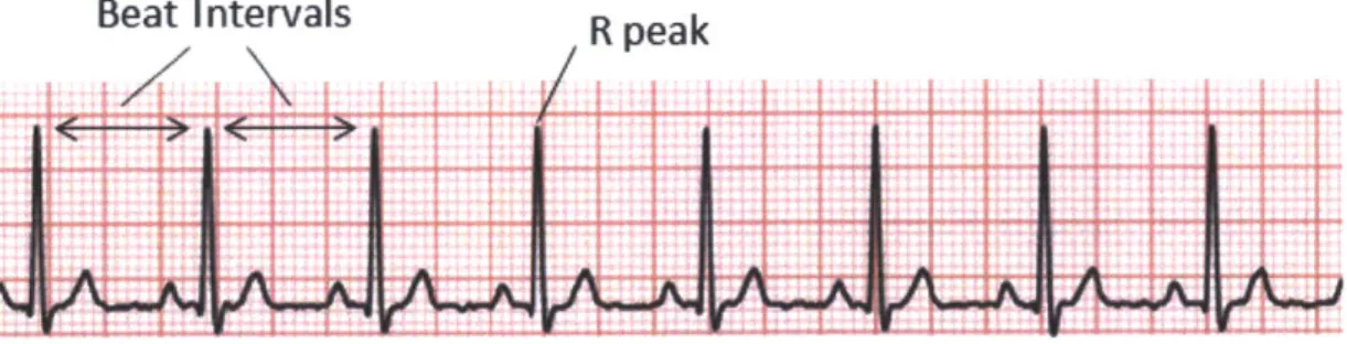
body of evidence [22] that measuring beat-to-beat variations provides additional in-formation with long-term prognostic value. The most established of these measures is heart rate variability (HRV). HRV measures the variation in the length of individ-ual normal (sinus) heartbeats. It provides an indication of the degree to which the sympathetic and parasymathetic nervous systems are modulating cardiac activity. To measure HRV, the interarrival times of beats must be accurately measured, which can be determined by locating the "R" peaks in successive beats in an ECG. A lack of sufficient variation when the subject is at rest suggests that the nervous system may not perform well under stress. Patients with decreased HRV are at an increased risk of adverse outcomes such as fatal arrhythmias.

Beat Intervals

_{R peak}

Figure 2-3: Example of typical ECG signal. Differences between R peaks in successive beats of an ECG can be used to calculate heart rate variability or HRV.

t

2.2

Optical Flow and the Lucas-Kanade Algorithm

Our approach relies on optical flow tracking to quantify the motion of a head in a video. Optical flow is the pattern of motion of objects, surfaces and edges in a visual scene. Optical flow methods try to calculate the motion of pixel locations between two image frames that are taken at times t and t + At. These methods are based on local Taylor series approximations of the image signal. For a 2D + t dimensional case a pixel at location (x, y, t) with intensity I(x, y, t) will have moved by Ax, Ay and At between the two image frames and the following image constraint equation can be given:

I(x, y, t) = I(x + Ax, y + Ay, x + Az) (2.1)

Assuming the movement to be small (subpixel or a few pixels in amplitude), the constraint can be rewritten using a Taylor series:

I(x+Ax,y+Ay,x+At)

=I(x,y,t)+ -AX+

Ay +

At

(2.2)

Dx Dy Dt

From these equations it follows that:

DI DI DI

_Ax+ Ay+ At=0 (2.3)

(x Dy (t

or

DIAx DIAy DIAt

±-+-

+- (2.4)

Dx At y At t At

This can be rewritten to form the optical flow equation:

IAV' + I7VY = -It (2.5)

where V, V, are the x and y components of the velocity or optical flow of I(x, y, t) and Ix, I, and It are the partial derivatives of the image at (x, y, t).

constant within a small neighborhood of the point p under consideration. The optical flow equation is made to hold for all points within the neighborhood and solutions to V, and V, are obtained using a least squares fit. In our work we use the Lucas-Kanade implementation provided in OpenCV [3]. This implementation is a sparse feature point tracker, meaning that it finds the motions of selected point locations in the image rather than finding a dense motion field for the entire image. The sparse tracker worked well for our application and is also much quicker than a dense optical flow algorithm.

For scenes with large motions, the Taylor approximation in Eq. 2.2 does not hold. In these cases one can use a coarse-to-fine optical flow scheme with image pyramids consisting of downsampled versions of the original images. The feature point velocities are refined from the coarsest image down to the finest (original) image. Since the motions we study are small, we did not use pyramids for our work.

RWd Channel Geen Chanel Blue Channel

Rud Skgnal Grae. SignaB SBue $gnu

Independent Component Analysis (ICA)

sopraO Swimu 1 Suetatod Suuicv 2 SeparaledSuren

Figure 2-4: Overview of color-based pulse detection method (image taken from [18]).

A face is found from the first video frame to construct a region of interest (ROI).

The red, green and blue channels are spatially averaged in the ROI in each frame to form three signals. ICA is applied on these signals to obtain three independent source signals. The most periodic source signal is chosen for analysis.

2.3

Color-Based Pulse Detection from Video

Blood circulation causes volumetric changes in blood vessels that modify the path

length of ambient light. This is the basic premise of plethysmography. The red, green, and blue (RGB) sensors of a video camera can pick up this plethysmographic signal mixed with other fluctuations of light caused by artifacts. In addition, because hemoglobin absorptivity varies across the visible spectral range, each of these sensors records a mixture of these sources with different weights. The task of pulse signal extraction is to reconstruct the signal of interest from these channels. A work that has gained recent interest separates the plethysmographic signal from the noise us-ing independent component analysis (ICA)[18]. The method (see Fig. 2-4) spatially averages the R, G, and B values from the facial area in each video frame to form three signals. Then, ICA is used to decompose the signals into 3 independent source signals. The source with the largest peak in the power spectrum is chosen as the pulse signal. Finally, the signal is smoothed and interpolated to 256 Hz for HRV analysis. When they evaluated their method on 12 subjects, they produced accurate heart rate and HRV measures.

Analysis of HRV was performed by power spectral density (PSD) estimation using the Lomb periodogram. They found the low frequency (LF) and high frequency (HF) powers which reflect different properties of the sympathetic and parasympathetic influences on the heart. The video recordings used in their analysis were roughly a minute in length, similar to the length of recordings in our work. However, this is a much shorter duration than the hours of ECG recordings used to calculate HRV measures in practice and it is not clear whether it is clinically meaningful. Therefore, in our work, we directly evaluate heartbeat length distributions instead of using the standard HRV measures.

Chapter 3

Method

Our method takes an input video of a person's head and returns a pulse rate as well as a series of beat locations that can be used for the analysis of beat-to-beat variability. We first extract the motion of the head using feature tracking. We then isolate the motion corresponding to the pulse and project it onto a ID signal that allows us to extract individual beat boundaries from the peaks of the trajectory. For this, we use

PCA and select the component with the most periodic ID projection. Finally we

extract the beat locations as local extrema of the chosen 1D signal.

Fig. 3-1 presents an overview of the technique. We assume the recorded subject is stationary and sitting upright for the duration of the video. We start by locating the head region and modeling head motion using trajectories of tracked feature points. We use the vertical component of the trajectories for analysis. The trajectories have extraneous motions at frequencies outside the range of possible pulse rates, and so we temporally filter them. We then use PCA to decompose the trajectories into a set of independent source signals that describe the main elements of the head motion. To choose the correct source for analysis and computation of the duration of individual beats, we examine the frequency spectra and select the source with the clearest main frequency. We use this criterion because pulse motion is the most periodic motion of the head within the selected frequency band. Average pulse rate is identified using this frequency. For more fine-grained analysis and calculation of beat durations, we perform peak detection in the time-domain.

(a). Region Selection Feature Tracking t=T (b). Trajectories x(t Y, W xN(t) JW (c). Temporal Filtering Frq Freq S (M) s2() WS (t) (f). Peak Detection (e). Component Selection

ECG ground truth

Figure 3-1: Overview of our pulse estimation approach. (a) A region is selected within the head and feature points are tracked for all frames of the video. (b) The horizontal and vertical components are extracted from each feature point trajectory. (c) Each component is then temporally filtered to remove extraneous frequencies. (d)

PCA decomposes the trajectories into a set of source signals s1, s2, S3, s4, s5. (e) The

component that has clearest main frequency is selected. (f). Peak detection identifies the beats of the signal.

Figure 3-2: The region of interest for subjects 1 and 2. The region encompasses the middle of the face.

3.1

Region Selection

We find a region of interest containing the head and track feature points within the region. For videos where the front of the face is visible, we use the Viola Jones face detector [27] from OpenCV 2.4 [3] to first find a rectangle containing the face. We use the middle 50% of the rectangle widthwise and 90% heightwise from top in order to ensure the entire rectangle is within the facial region. We also remove the eyes from the region so that artifacts caused by blinking do not affect our results. To do this we found that removing the subrectangle spanning 20% to 55% heightwise works well

(see Fig. 3-2). For videos where the face is not visible, we mark the region manually.

3.2

Feature Point Selection

We measure the movement of the head throughout the video by selecting and tracking feature points within the region. We use the OpenCV Harris corner detector (the

goodFeatures To Track function) to select the points. We set the parameters of this

3.3

Feature Point Tracking

We apply the OpenCV Lucas Kanade tracker between frame 1 and each frame t =

2 - T to obtain the location time-series (xn(t), ys(t)) for each point n. We used a

window size of 40 pixels around each feature point for tracking. This window size is

1 the area of the face rectangle found by the detector for our subjects on average.

125

It is large enough to capture local features around the nose/mouth area.

Many of the feature points can be unstable and have erratic trajectories. To retain the most stable features we find the maximum distance traveled by each point between consecutive frames and discard points with a distance exceeding the 7 5th

percentile.

3.4

Temporal Filtering

Not all frequencies of the trajectories are useful for pulse detection. A normal adult's resting pulse rate falls within [0.75, 2] Hz, or [45, 120] beats/min. We found that frequencies lower than 0.75 Hz negatively affect our system's performance. This is because low-frequency movements like respiration and changes in posture have high amplitude and dominate the trajectories of the feature points. However, harmonics and other frequencies higher than 2 Hz provide useful precision needed for peak de-tection. Taking these elements into consideration, we filter each x,(t) and y,(t) to a passband of [0.75,5] Hz. For babies, who have faster pulses, we use a passband of

[1.25, 5] Hz. We use a 5th order butterworth filter for its maximally flat passband.

3.5

PCA Decomposition

The underlying source signal of interest is the movement of the head caused by the cardiovascular pulse. The feature point trajectories are a mixture of this movement as well as other motions caused by sources like respiration, vestibular(balancing) activity and changes in facial expression. Each subject exhibits different motions. Fig. 3-3 shows examples of the total energy of the feature point trajectories at different

2.5

05 2 35 1 4 1 2 3 4 5 0 1 2 3 4 5

a. b. c. d.

Figure 3-3: Examples of the combined energy spectra of feature points for 4 different subjects. (a) is an example where the pulse frequency is the only dominant frequency.

(b) is an example where there is another frequency with nearly as much energy as

pulse. (c) is an example where the harmonic of the pulse frequency has more energy than the pulse frequency. (d) is an example where the energy at the pulse frequency is smaller than several other peaks in the spectrum. We were able to get accurate pulse signals for all subjects using our method which separates the combined motion of the feature points into submotions using PCA.

frequencies for four different subjects. The black arrow indicates where the true pulse rate is. In the first case (a), the dominant frequency corresponds to pulse. This is the easiest case. In the second case (b) the pulse still has maximum energy but there is another frequency with nearly as much energy. In the third case (c), the harmonic of the pulse has greater energy than the pulse itself. In case (d) the pulse is completely masked by extraneous motions. The task of developing a method to extract a reliable pulse for these different cases is challenging.

Our task is to decompose the mixed motions of the feature points into subsignals to isolate pulse. To do this we consider the multidimensional position of the head at each frame as a separate data point and use PCA to find a set of dimensions along which the position varies. We then select a dimension on which to project the position time-series to obtain the pulse signal.

Formally, given N feature points, we represent the N-dimensional position of the

head at frame t as mt = [x1(t), x2(t), - - -, XN(t), Y1(t), Y2(t), * .

,yN(t)].

and the covariance matrix of the positions are defined by:

I T

(3.2)

PCA finds the principal axes of variation of the position as the eigenvectors of

Em(bm = <bmAm (3.3)

where Am denotes a diagonal matrix of the eigenvalues A1, A2

,-ing to the eigenvectors in the columns of 4 m, 01, 02, -

,ON-0p

- AN

correspond-'P2

Figure 3-4: Examples of the first three eigenvectors for two subjects. Each white arrow on a face represents the magnitude and direction of a feature point's contribution to that eigenvector. The eigenvector decomposition is unique to each video.

TI

Fig. 3-4 displays the first three eigenvectors for two of the subjects. Each

eigen-vector represents the 2N-dimensional direction and magnitude of movement for the feature points. The eigenvectors differ for each video. We obtain the 1-D position signal si(t) by projecting the position time-series onto O4 :

Si(t) 2

i(.)

mT

There are periods in the video during which the head moves abnormally (e.g. swallowing, adjustments in posture). Such movement adds variance to the position vectors, thereby affecting the PCA decomposition. To deal with this we discard a percentage a of the mt with the largest L2-norms before performing PCA. However, all of the mt must still be used in the projection step (Eq. 3.4) to produce a complete signal. We set a at 15% for our experiments.

A popular alternative to PCA is independent component analysis (ICA), which

decomposes signals based on higher order statistics. We did not see any improvement in our results when using ICA.

3.6

Signal Selection

The question remains of which eigenvector to use for pulse signal extraction. The eigenvectors are ordered such that q1 explains the most variance in the data,

#

ex-plains the second most, and so on. Fig. 3-5 shows the percentage of total variance attributed to the first 5 eigenvectors averaged over all subjects. The first two eigen-vectors account for 56% and 36% of total variance on average. This makes intuitive sense when looking at Fig. 3-4, which shows that the first two components tend to capture most of the horizontal and vertical motions of the head. However, this does not mean that s, or s2 is the clearest signal for analysis. In fact, it is likely that these

with pulse motion. 70 60 50 40 30 0 20 10 0 1 2 3 4 5 PCA component

Figure 3-5: Percentage of total variance explained by the first five PCA components, averaged over all subjects in our experiments. Bars are standard deviations. The first component explains most of the variance for all subjects. However, the first component may not produce the best signal for analysis.

We instead choose the eigenvector

#1

energy at

j

We found it unnecessary to consider any signals beyond the first five, i.e. s1, ..., S5

for any of our subjects. We label the maximum frequency of the chosen signal as

fpuise and approximate the pulse rate as 60 * fpulse beats per minute.

For the 18 subjects in our experiments the first five components were chosen the following number of times: 3, 1, 13, 1, and 0. The third component was chosen for

14 of the 18 videos. We hypothesize that this is because the first two components remove much of the extraneous motions as seen in Fig. 3-3 leaving a purer residual motion for the third component to capture.

3.7

Peak Detection

Pulse rate alone is not, of course, sufficient to fully evaluate the cardiovascular system. Clinicians often assess beat-to-beat variations to form a more complete picture. To allow for such analysis, we perform peak detection on the selected PCA component signal. Since a modern ECG device operates around 250 Hz to capture heart rate variability and our videos were only shot at 30 Hz, we first apply a cubic spline interpolation to the signal to increase its sampling rate to 250 Hz.

The peaks are close to 1 seconds apart with some variability due to the natural fpulse

variability of heartbeats, variations of the head motion, and noise. We label each sample in the signal as a peak if it is the largest value in a window centered at the sample. We set the length of the window (in samples) to be round( 250

).

shows examples of signals outputted by our method. Peaks are marked by circles.

Figure 3-6: Examples of motion signals outputted by our method. Red circles are peaks.

Chapter 4

Experiments

We implemented our approach in MATLAB. Videos were shot with a Panasonic Lu-mix GF2 camera in indoor, unisolated environments with varying lighting conditions.

All videos had a frame rate of 30 frames per second, 1280 x 720 pixel resolution

and a duration of 70-90 seconds. Videos were saved in MJPEG format. During the recordings, subjects were told to sit still as possible while looking forward at the camera (for frontal videos) and away from the camera (side/back views). Fig. 4-1 shows frames from frontal videos of all 18 subjects. The subjects varied in gender (7 female, 11 male) and skin color. They ranged from 23-32 years of age and were all seemingly healthy. We connected subjects to a wearable ECG monitor [5] for ground truth comparison. This device has a sampling rate of 250 Hz and three electrodes that we placed on the forearms.

4.1

Visible Face

We extracted pulse signals from the 18 subjects with a frontal view of the face (Fig.

4-1). We calculate our program's average pulse rate using the frequency of maximal

power for the selected PCA component. Similarly, we compute the true pulse rate

by finding the main frequency of the ECG spectrum. Table 4.1 presents our results.

The average rates are nearly identical to the true rates for all subjects, with a mean absolute difference of 1.4%. The number of peaks were also close to ground truth

1 2 3 4 5 6

7 8 9 10 11 12

13 14 15 16 17 18

Figure 4-1: Reference frames from videos of all 18 subjects. Subjects varied in skin color, gender and age.

values, with a mean absolute difference of 2.1%.

We also evaluate the ability of our signal to capture subtle heart rate variability. Clinically meaningful HRV measures typically use 10-24 hours of ECG data. There-fore we did not attempt to compute any of these for our 90 second videos. Instead, we compare the distributions of time between successive peaks for each signal. Incorrect or missed peaks can introduce spurious intervals too large or small to be caused by

the natural variations of the heart. We account for these cases by only considering intervals with a length within 25% of the average detected pulse period.

We use the Kolmogorov-Smirnov (KS) test to measure the similarity of the dis-tributions, with the null hypothesis being that the observations are from the same distribution. Table 4.1 presents the results. At a 5% significance level, 17 of the 18 pairs of distributions were found to be similar. Fig. 4-2 presents histograms of 5 of

Table 4.1: Results when comparing the beat length distributions of the ECG and our method. Presented are the means (y) and standard deviations (o-) of the distributions along with p-value of the Kolmogorov-Smirnov test measuring distribution similarity.

17 of the 18 pairs of distributions were not found to be significantly different (p >=

0.05) Sub. 1 2 3 4 5 6 7 8 9 10 11 12 13 14 15 16 17 18

ECG Motion Similarity

Pulse Rate # of beats A(a) Pulse Rate # of beats p0) p-value

(% err) (% err) (high is good)

66.0 55.3 81.3 44.0 95.3 78.0 73.3 59.3 56.6 78.9 84.6 63.3 60.0 60.7 80.7 74.7 50.0 78.0 99 83 122 66 143 91 110 89 85 100 127 95 90 91 121 112 75 91 0.91(0.06) 1.08(0.08) 0.73(0.04) 1.34(0.19) 0.62(0.03) 0.76(0.04) 0.81(0.05) 1.01(0.04) 1.04(0.07) 0.75(0.04) 0.70(0.06) 0.94(0.08) 0.99(0.04) 0.98(0.11) 0.74(0.05) 0.80(0.05) 1.18(0.08) 0.77(0.05) 66.0(0) 56.0(1.2) 82.7(1.7) 46.0(4.6) 96.0(0.7) 78.9(1.2) 72.0(1.8) 58.7(1.1) 58.7(3.6) 82.1(4.1) 85.3(0.8) 62.7(1.0) 60.0(0) 60.7(0) 81.3(0.8) 76.0(1.8) 50.0(0) 78.9(1.2) 99(0) 82(1.2) 119(2.5) 66(0) 143(0) 91(0) 98(10.9) 89(0) 83(2.4) 98(2.0) 116(8.7) 95(0) 90(0) 87(4.4) 117(3.3) 110(1.8) 75(0) 90(1.1) 0.91(0.07) 1.09(0.10) 0.73(0.08) 1.33(0.19) 0.62(0.07) 0.76(0.04) 0.83(0.06) 1.00(0.10) 1.04(0.12) 0.75(0.04) 0.71(0.07) 0.94(0.09) 0.99(0.08) 0.99(0.12) 0.75(0.06) 0.80(0.05) 1.19(0.10) 0.77(0.07) 0.78 0.96 0.16 0.92 <0.01 0.94 0.14 0.06 0.34 0.60 0.57 0.72 0.27 0.74 0.62 0.87 0.85 0.22

the 16 distributions binned at every 0.05 seconds. Our method was able to capture a wide range of beat-length distributions shapes, from the flat distribution of subject 4 to the peakier distribution of subject 16. Fig. 4-2 also shows the distribution pair for subject 5's video, which the KS test labeled statistically dissimilar. Our distribution is more normally distributed than the ECG distribution. Subject 5's heart rate, 1.6

Hz, was the highest heart rate in our test set. At high heart rates the duration of each beat is small, meaning that variation between beats is also small. We believe that our method struggled because of this.

4.1.1

Motion Amplitude

Pulse motion constitutes only a part of total involuntary head movement. We quantify the magnitude of the different movements within [0.75, 5] Hz by calculating root mean square (RMS) amplitudes of the feature point trajectories.

Subject 4 E CG Motion Subject 1 EG Motion Ca Oh Subject 17 ECG CIA 00 0: 1I U It Motion Subject 16 ECG OIL all Motion

OLL

x-axis istime (sec), y-axisisfractionof tool beats

Figure 4-2: Beat distributions of the ECG and our motion method for subjects. (a) We were able to accurately capture a wide range of distribution shapes, such as for subjects 4, 17, 1 and 6. (b) We were not able to produce an accurate distribution for subject 5.

Table 4.2: Mean (std. dev.) RMS amplitudes in pixels for the x and y feature point trajectories for all subjects. Values are shown after filtering to within 0.05 Hz of the pulse frequency (RMS Pulse) and without filtering (RMS Total).

RMS Pulse RMS Total RMS Pulse

RMS Total

X 0.17(0.11) 0.44(0.05) 0.36

y 0.11(0.05) 0.29(0.08) 0.38

Table 4.2 presents the amplitudes averaged across all subjects, with the x and

y trajectories averaged separately. We calculated the mean amplitude after filtering

within 0.05 Hz of each subject's pulse frequency (RMS Pulse) and without filtering (RMS Total). The x axis had larger pulse and total motion amplitudes, but the ratio between the two was slightly higher for the y axis. For both the x and y axes the pulse amplitude was less than 40% of the total amplitude, indicating that factors other than pulse cause a majority of head motions when a person is sitting still - even when only considering the frequency band [0.75,5] Hz.

4.1.2

Noise Analysis

Original 50 100 200 400 500

Figure 4-3: Frames from videos of subject 1 with varying levels of additive gaussian noise. The top row shows frames before filtering. The bottom row shows frames after bilateral filtering. Noise ranged from a standard deviation of 5 to 500 pixels. Bilateral filtering smooths images while retaining edges.

We performed noise analysis to evaluate the robustness of our system. We added zero-mean Gaussian noise to the videos, sweeping the standard deviation cros from

5 to 500 pixels. The noise was added to each channel independently. To smooth

the noise we applied a bilateral filter [24] to each frame of the noisy videos. The bilateral filter is a smoothing filter that preserves edges and corners, which can be useful for tracking. The intensity value at each pixel in an image is replaced by a weighted average of intensity values from nearby pixels, with weights depending on both Euclidean and intensity differences. Formally, the intensity of pixel p is replaced

by:

W EGod(I|p

- qJ|)Ga,(||Ip

Iq||)Iq

(4.1)

WPq,

where Ip is the current intensity at p, Iq is the intensity at each pixel q, G,, and G, are Gaussian functions depending on Euclidean and intensity differences, and W, is

a normalization factor. We set Ocd = 3 and a, = Unoise. Fig 4-3 shows frames from

videos of subject 1 with different levels of noise before and after applying the bilateral filter.

For each subject we found gmaxnoise, the maximum noise standard deviation before

our method first produced an average pulse rate outside 5% of the true rate. Bilateral filtering resulted in a better (larger) 0maxnoise for 16 of the 18 subjects, worse

perfor-mance for 1 subject, and no change in perforperfor-mance for 1 subject. Overall, filtering improves our method's performance against noise. Therefore, the rest of our results

are compiled using bilateral filtering.

Fig. 4-4a presents 0maxnoise for each subject. There is a large variance in 0-maxnoise

across the subjects. Fig. 4-4b plots the number of distributions of beat lengths that are similar to ground truth (using the KS test) as anoise is increased. Most of the

17 distributions that were initially found to be similar to ground truth are dissimilar

when 7noise ~ 50.

The large variance in Omaxnoise suggests that there are video-specific factors that affect performance. We hypothesized that the variance is caused by two video-specific factors: strength of head motion and feature point quality. A video with large and clear head motions related to cardiac activity should result in a higher Omaxnoise. A

video with feature points on good image patches, i.e. patches with high gradients, should result in less tracking error, which also leads to a higher 0maxnoise. We tested these hypotheses by quantifying motion strength and feature point trackability with metrics. The metrics are based on the original videos (without added noise), and we test whether they have any correlation with 0maxnoise.

We developed two metrics measuring motion strength. The first, which we call 3, is the difference between the total energy of the feature points at fpuse to the maximum total power at any other frequency outside 0.05 Hz of the pulse frequency.

#

If the energy at the pulse frequency is barely larger or even smaller than the energy

at another frequency, 3 will be small. It is possible for

#

20 400 3505 230 0 5 10 15 20 0 100 200 300 4O 50 Sa0bect (a) (b)

Figure 4-4: Plots presenting results after adding varying levels of Gaussian noise to our videos. (a) shows clmaxnoise, the standard deviation of the first noise level at which

our method gave an incorrect average pulse rate. (b) shows the number of similar distributions reported by the KS test as noise is added to the videos.

Fig. 3-3 this is possible when the harmonic frequency is large or when there is strong periodic component corresponding to other body movement. The second metric, -y is based on the PCA decomposition of the feature point trajectories of the original video. -y is a weighted sum of the variance of each PCA signal si with main frequency

fi ~~ fpulse:

5

=

S

fil

The weight for each si is the periodicity metric pi that we defined earlier in Chap-ter 3. A signal with large amplitude (high A) and large periodicity (high p) will result in a high -y value. Fig. 4-5 shows our results comparing ormaxnoise to

#

and -y have a significant positive correlation with -maxnoise (Pearson R coefficients of

0.83, 0.76, p values < 0.01). This suggests that the strength and clarity of the head

motions are contributing factors to noise performance.

Next, we wanted to determine the effect of feature point quality on gmaxnoise. We quantify feature point quality, rK, as the variance of the luminosity intensity within the 40 x 40 pixel window surrounding the point. This window size is the same size we

500 - 2 500 2 450 450 400 400 13 13 350 * *9 350 09 300 #15 300 15 250 05 .*3 250 *3 200 12*014 200 )0 42 14 10 150 016 R 0.77, p < 0.01 150 *16 R= 0.83, p < 0.01 100 177100 *. *7 47 011 07 50 8 6 1 _{50 418} * 18 6 1 0 *0 -0.5 0 0.5 1 1.5 2 2.5 0 0.1 0.2 0.3 0.4 0.5 0.6 0.7 x10

Figure 4-5: Plots of Omaxnoise VS.

3

Omaxnoise-used for the Lucas-Kanade tracker. Intuitively, a low variance indicates a featureless or poor region. Fig. 4-6a shows a heatmap of r, on a frame of subject 3's video, with red being the highest quality. Locations near the mouth and nose have high K while the cheeks and forehead do not.

First, we explored how r, relates to tracking error. We measured the tracking error for each feature point on the videos. The tracking error at a frame is the distance between the point's location in the noiseless video and its location in the noisy video. Fig. 4-6b plots the average RMS tracking error of the feature point trajectories binned at different values of K for each noise level. We see a clear negative relationship

between tracking error and K. for all noise levels, as expected. However, at higher noise levels even the best points have quite a large tracking error, indicating that points are drifting in location over time. Despite this relationship between r and tracking error, we were unable to find any relationship between the average r, for a video and Omaxnoise (see Fig. 4-6c).

We ran a final experiment testing whether selecting a small subset of high quality feature points will result in a larger Omaxnoise. We added a varying number of feature

300 r

IU

(a) A heatmap of , for a frame

of subject 3's video. Hotter col-ors (e.g. red) indicate high K

while coolor colors (e.g. blue) indicate low r. The best K

within the feature point region is near the nose and mouth.

200 1SO 100 500 450 4 2.50 2M0 -150 125 100 75 50 0 500 1000 1500 2000 2500 3000

(b) Average root mean square tracking error of

fea-ture points for all subjects binned at different r values. Each line corresponds to a different noise level (cnoise

is indicated next to each line). Larger K results in lower

tracking error for all noise levels.

500 450 400 350 300 250 200 150 e2 9 . *13 15 05 *14 *10 s12 016 100 1107 50 06 8018 0 200 400 600 800 1000 Average x 017 1200 1400 1600

(c) Plot of Omaxnoise vs. average K in a video. The

variables are not significantly correlated.

Figure 4-6: Analysis of K, our metric measuring feature point quality.

0

points with high

r,

N,

all subjects for each level. For comparison, we also show results when only selecting points with low K and selecting points randomly within the region of interest. For the random selection we selected 10 random sets of feature points and record the average

(maxnoise. The results of this experiment show that selecting points randomly and by

high , yields similar results. Selecting points with low K performed predictably poorly. Adding more feature points increased performance in all scenarios but helped low K the most. Increasing the number of feature points from 150 to 1500 only increased

0maxnoise by 30 when selecting points randomly or by high ii.

200 180 J 160 140 120 40 60

p....

Number of feature points

Figure 4-7: The average Omaxnoise of all subjects vs. the number of feature points

selected. 1500 points is the number of feature points used in the original results (see Fig. 4-4a). We selected points in three ways: randomly around the region of interest,

by the highest r and by the lowest K. The random results were repeated 10 times

and averaged. Random selection and the high K selection peformed similarly while low K yielded the worst results. Adding more feature points increased 0maxnoise for