Analytical verification of undesirable properties of direct model reference adaptive control algorithms

ANALYTICAL VERIFICATION OF UNDESIRABLE PROPERTIES OF DIRECT MODEL REFERENCE ADAPTIVE CONTROL ALGORITHMS*

by

Charles E. Rohrs, Lena Valavani, Michael Athans and Gunter Stein

Laboratory for Information and Decision Systems Massachusetts Institute of Technology

Cambridge, Massachusetts 02139

ABSTRACT

In the past few years many model reference adaptive control algorithms have been shown to be globally asymptotically stable. However, there have been no analytical results on the performance of such systems in the transient adaptive phase. Simulations have shown that there are three particular problem areas in which the performance of these

algo-rithms may be unsatisfactory when viewed from a practical context. The pro-blems are (a) the generation of high frequency control inputs, (b) high susceptibility to instability in the presence of unmodeled dynamics, and (c) poor performance in the presence of observation noise. This paper displays analytically how these problems arise for a number of algorithms. The analysis technique employs linearization of the non-linear time varying dynamic equations that describe the closed-loop system; this analysis technique is referred to as "final approach analysis" because the linearization is valid when the system and ref-erence model outputs are close to each other, a fact that occurs during the final phases of adaptation. By studying simple first order systems one can analytically examine different adaptive algorithms, and pinpoint

their shortcomings. However, the analytical studies are constructive because they indicate how to modify the algorithms so as to improve

their practical utility. Also, a proof is given that one of the algo-rithms studied is output and parameter error mean-square stable in the presence of white observation noise.

*This research was supported by the Air Force Office of Scientific Research under grant AF-AFOSR-77-3281 and by the NASA Ames Research Center under grant NGL-22-009-124.

*This paper has been submitted for publication to the IEEE Trans. on Automatic Control: it has been accepted for presentation at the 20th

1. INTRODUCTION

During the past few years globally asymptotically stable model reference adaptive control (MRAC) algorithms have been developed both in continuous time [1]-[4] and discrete time [5]-[8]. These algorithms have been designed with the sole purpose of attaining asymptotic model following with no regard for the transient performance of the resulting adaptive control system. This is in apparent contrast with the original motivation for introducing a

linear reference model as part of the overall adaptive design (MRAS). The reason for introducing the model was precisely to force the adaptive system not only to follow asymptotically the desired model output but also to have comparable transient characteristics to those of the prescribed model. More-over, such closed loop adaptive algorithms result in non-linear (time-vary-ing) systems whose transient characteristics can have very complex and un-desirable behavior. [9] This paper provides the first definitive attempt

and results towards establishing analytically the performance of these algorithms viewed from a practical control design point of view.

A simulation study of the algorithm of [1], originally reported in [9] and reviewed in Section 2 of this paper, pointed to three undesirable char-acteristics from which such algorithms may suffer. These problems are:

* the generation of high frequency control inputs

* high susceptibility to instability in the presence of unmodeled dynamics

* poor performance in the presence of observation noise.

In order to demonstrate these problems analytically, this paper makes use of what will be called a final approach analysis. The adaptive control system is studied only for the case where the parameters and closed loop

output are already close to their "desired" values.

Various algorithms are analyzed using only a nominally first-order

plant although the results do generalize to higher order systems, and such

generalizations are under way. The plants and models used for both

con-tinuous and discrete time systems are given in Section 3.

Sections 4 and 5 contain the analysis for the continuous and

discrete-time algorithms respectively in the case of noise-free observations. The

undesirable characteristics observed in the previous simulations [9] are

demonstrated analytically and some insight as to what causes them is attained,

The basic problem is that large reference inputs force the adaptive system

to try to react too quickly. This results in a large bandwidth system and

consequently in the excitation of unmodeled dynamics, which brings about

instability. It is shown in Section 5.2 that the modifications of [3]

developed in [6] and [7] provide enough flexibility to improve behavior in

the final approach if the parameters of [7] are chosen according to the

procedure given in that section.

Section 6 displays analytically the adverse effects of observation

noise discovered in the simulation studies [9]. General comments are made

there as to how this noise can be dealt with. Section 7 also provides a

proof that the algorithm of Section 5.1 is mean square stable in both the output and parameter errors in the presence of white observation noise.

Section 8 contains the conclusions.

It should be noted that only direct model reference algorithms are

treated in this paper. Indirect approaches, such as in [10] and [11],

usually require parameter convergence for proof of stability. It is not

clear what such a condition implies when the plant has at least one

un-modeled pole. Identification in such cases with unun-modeled dynamics is

actual input to the process is the sum of a (known) reference input and of

dynamically evolving adaptive signals (parameter and filtered state variables)

identification in the presence of unmodeled dynamics is an important

un-resolved question at the present time. The "sufficient excitation"

condition required for identification in [10] and [11] cannot be guaranteed

globally, but even if this were the case, its adverse effects on the

over-all adaptive system stability properties could be of more considerable concern.

All the algorithms considered suffer (more or less) from the same basic

problem: they lead to high-gain designs with large bandwidths. Hence,

un-modeled dynamics can be excited and the adaptive system can become unstable.

Unfortunately, simple pragmatic cures such as

(a) passing the control signal through one or more low pass filters

to insure rapid rolloff, and

(b) low-pass filtering of the noise corrupted measurement signals are not guaranteed to work, because the presence of the additional rolloff

and low-pass dynamics violate the relative degree assumptions that are

neces-sary to prove the global stability of this class of algorithms. Also, the

current theoretical framework cannot be used directly to obtain a class of

adaptive algorithms that exploit partial knowledge of the controlled plant

dynamics (e.g. the roll-off and noise filter transfer functions). Thus, analytical studies such as these reported in this paper are

absolutely necessary to understand the properties and limitations of adaptive

control algorithms. The results presented represent only a small initial

step; a great deal of additional research is needed to generate new adaptive

algorithms that are robust in the presence of stochastic and modelling-error

2. REVIEW OF THE SIMULATION RESULTS

In [9] the results of the digital simulation of the algorithm of [1 ] Were presented. The plant used was a simple second order system with one

zero. In addition to offering insights into the convergence behavior of the adaptive process, the study pointed to three serious problems in the adaptive algorithm simulated--problems which in this paper are shown to be inherent in many if not all of the theoretically globally stable adaptive control algorithms presented in the literature to date. The results of the simulation are reviewed here since the major focus of this paper is to explain these results analytically and to offer improved solutions to them.

First, it was shown that even when the system was properly modeled, the plant was subjected to substantial amounts of high frequency control inputs. High frequency inputs are clearly undesirable as they can excite unmodeled dynamics and may also lead to instability and actual failures in some plants.

Second, it was observed that in the presence of an unmodeled pole the controlled plant exhibited wildly oscillatory and even unstable closed loop behavior.

Third, it was shown that in the presence of a small amount of observation noise the closed loop system did not converge to the model but would slowly drift away to an increasingly higher bandwidth system.

3. THE SYSTEM MODEL 3.1 The Nominal Case

The adaptive algorithms studied in this paper all display the undesirable characteristics discussed in Section 2 even when the process to be controlled is assumed to be first order. In the continuous-time case the system to be studied can be represented by the following set of differential equations:

Actual Plant: y(t) = - ay(t) + Bu(t) (1.a)

Reference Model: y*(t) = - ay*(t) + br(t) (l.b)

where a and 8 are the unknown but constant parameters of the plant to be controlled, a and b describe the known model dynamics, with a > O, b > 0, r(t) is a reference input, and u(t) is a control input to be chosen in such a way as to make the output of the plant, y(t), follow that of the reference model, y*(t). Similarly, in discrete-time the plant-model representation is given by

Actual Plant: y(t+l) = ay(t) + 8u(t+l) (2.a)

Reference Model: y*(t+l) = ay(t) + br(t+l) (2.b)

where lal < 1, b > 0 and all the other quantities are defined in complete analogy with the continuous time case. Different adaptive algorithms can then be employed in a recursive choice of the control input u(t).

3.2 Unmodeled Plant Dynamics

In order to investigate the effects of unmodeled dynamics on a

particular adaptive control algorithm, the actual plant is augmented to have two poles, located at - al and -a2 respectively. Its continuous-time

dynamics now evolve according to

(t)+ (i+a ₂)Y(t) + a₁a₂y(t) = Bu(t) (3.a)

Then an adaptive controller is designed based on the assumption of a first

order plant which has to match the output of a desired model still described

by (l.b). This is obviously very hard to do for arbitrary reference inputs.

For the purpose, however, of demonstrating the problems that arise when one

deals with plants with unmodeled dynamics consideration of constant inputs

sufficesto carry through the analysis.

Further, in order to proceed with the analysis in this paper, it is also

assumed that there exists a second order model with poles at -a₁ and -a₂

described by the differential equation

Y*(t) + (a1+a2)y*(t) + ala2y*(t) = b2r(t) (3.b)

with the following conditions satisfied:

(i) the system (3.b) is stable

(ii) al + a2 of eqn.(3.b) is equal to al + a2 of eqn. (3.a)

(iii) the system described by eqn. (3.b) has the same dc gain as

that in eqn. (l.b), i.e. b₂/ala₂ = b/a.

Conditions (i) and (iii) allow the substitution of eqn. (l.b) with eqn. (3.b)

with no change in (steady-state) response for constant reference inputs.

Condition (ii) is necessary for the analysis and is somewhat restrictive

in the plants and models that can be studied comparatively.

the unmodeled pole. The conditions on eqn. (3.b) can be met if a2 > 0 and

[a2[ > jall. This is true if a2 represents a stable high frequency unmodeled

pole. If

1a21

is much greater than both

Iall

and

jai

in eqn. (l.b), then

a1 of ieqni (3.b) can be set equal to a in eqn. (l.b). This results in

a2 = a2 + al - a still being a large number, so that the output of eqn. (3.b) will match the output of eqn. (l.b) over a substantial frequency range of

reference inputs.

Thus, although the analysis in this paper is performed, for the most

part, only for constant reference inputs, it is valid over the range of

reference input frequencies where (3.b) matches (l.b). A point to be made

here is that, if the controller is forced to be too fast--i.e. a is too

large--, increased sensitivity to unmodeled poles will result, since in

that case it will become more difficult to satisfy condition (ii).

A completely analogous set-up is used to study the effects of unmodeled

dynamics in the discrete-time case. Now the plant and model are described

respectively by

Actual Plant: y(t+2) - (al1+a2)Y(t+l) + ala2y(t) = Bu (t+2) (4.a)

Reference Model: y*(t+2) - (al+a2)y*(t+l) + ala2y*(t) = b2r(t+2) (4.b)

The corresponding conditions on eqn. (4.b) are:

(i) The plant (4.b) is stable. (ii) al + a2 = 1 + 2

2 b

(iii) + ala2 of eqn (4.b) = of eqn. (2.b)

2-(a 1+a

Condition (ii) on eqn. (4.b) is in some sense more restrictive than the

same condition on its continuous-time counterpart. If the poles of the

discrete time system are restricted to the positive real axis,i.e. the

discrete time system arises from fast enough sampling of a continuous-time

system with its poles on the real axis, and if a1 > 2, then conditions (i) and (ii) on eqn. (4.b) cannot be met regardless of how high a frequency the

unmodeled pole a2 is. However, if the system is indeed derived by sampling a continuous-time system where the unmodeled pole is at a higher frequency

than the modeled pole, the problem can be alleviated by sampling the system

faster which will bring the discrete-time modeled pole in to a value closer

to 1 than the unmodeled pole.

The point made in the continuous time system discussion about forcing

the controller to be too fast assumes more importance here as one of the

algorithms studied attempts to perform dead-beat control,i.e. it sets

a, = 0. In this case conditions (i) and (ii) cannot be met if the plant is unstable.

4. FINAL APPROACH ANALYSIS OF SOME CONTINUOUS TIME ADAPTIVE ALGORITHMS In this section it will be shown that the continuous time algorithms studied possess undesirable characteristics even under the restrictive assumptions of final approach analysis. In the final approach analysis it is assumed that the parameters of the controlled plant are very close to those parameters which would make the closed loop characteristics of the process the same as those of the reference model. Such a situation could develop when the asymptotically stable adaptive controller has already been operating for a long period of time with sufficiently rich inputs and therefore is close to final convergence. It could also arise when the plant parameters are fairly well known under reasonable a priori knowledge of the plant parameter values and the adaptation is just employed as a fine-tuning mechanism. Surely, if an algorithm behaves poorly under these mild con-ditions, it certainly cannot be expected to be useful as a practical control design.

4.1 The Algorithm of Narendra-Valavani [1] and Feuer-Morse [2]

The algorithms of[l] and [2] are the same in the case where the relative degree (the number of poles minus the number of zeros) of the actual plant is one, asis the case with the system considered here. This was the algo-rithm used to produce the simulation results discussed in Section 2 and the findings of this subsection will explain some of the remarks of Section 2 analytically.

According .to the formulation in [1] with the first order model.of..Section 3., the control input u(t) is equal to

= ~ [(a-a+%l(t))y(t) _{+ (b+4 2(t))r(t)] (5)}

where 61(t), 02(t) are the adjustable controller parameters and _l(t),

¢2(t) _{are the parameter errors. The adaptive algorithm in [1] adjusts the} parameters e₁(t), 0_{2(t) according to eqns. (7.c) and (7.d) in the sequel.} When ~1 = ~2 = 0 _{the controlled plant will match the reference model as} is obvious by observation of eqn. (5). The output error is defined as

e(t) = y(t) - y*(t) ₍₆₎

The nonlinear time-varying equations associated with the adaptive algorithm can then be expressed as functions of the state and parameter errors as follows:

y(t) = -ay(t) + 0l(t)y(t) + 02(t)r (7.a) e(t) = -ae(t) + l(t)y(t) + 4₂(t)r _(7.b)

1t) ( = -Yl lY(t)e(t) - y re(t) _(7.c)

M 1(t) = 8 ₁₂

Xl(t)

02(t) = = _{-y 2 1y(t)e(t) - y}

2 2re(t) (7.d)

where the yij's are the adaptive gains. Equation (7.b) results from eqns.(l), (5),and (6) while eqns. (7.c) and (7.d) are determined by the choice of the particular algorithm, in this case that in [1]. Choosing

the gain matrix Fr

IY1

rT>

in [1] and [2] that lim e(t) = 0 and that ~₁

(t)

4.1.1 Final Approach Analysis with Proper Modeling and Constant Reference Input

To use the final approach analysis in eqns. (7) we assume that e(t),

~l(t), and ¢₂(t) are small compared to y*(t) and r(t). Linearizing the system (7) around the point e = c1 = ~2 = 0 yields the linear system

1e

-

-a

BY*

r

er

dt

=

ly-

r

O

2/

Y*-

r

0

0

I

2/[

l

If r is assumed to be constant, y* will also be constant and the system

(8) will become a linear time-invariant system whose characteristic equation

is given by:

s(s2 + as + d*) =

0

where

d* = Y₁Y*2 + (Y12 + Y2 1)y*r 22r (10)

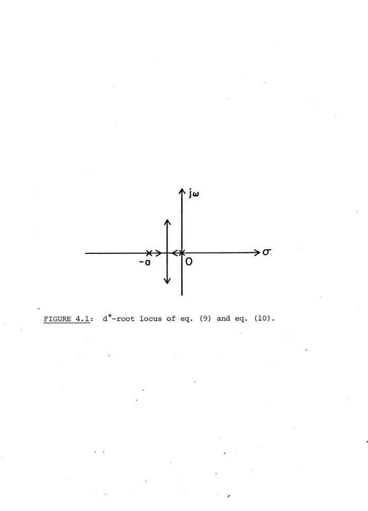
One pole of this system (8) remains fixed at the origin, while the other

two can be thought of as being determined by a root-locus pattern associated

only with the (s2 + as + Sd*) part of (9) using d* as the gain parameter as in Figure 4.1. The diagram of Figure 4.1 will be referred to as the d*-root

locus of eqn. (9).

From Figure 4.1 and eqn. (10) it is seen that for large reference

FIGUR

4.1:

(9) and eq. (10)

d-root

locus

of

eq.

errors and also, through eqn. (5),in the plant input u(t). Thus, the high

frequency control inputs observed in the simulations described in Section 2

will be present for large reference input values even when this input is

constant, the plant is first order, and the adaptation process is in the

final approach to convergence.

The pole that is fixed at the origin is associated with the eigenvector

e = 0, (11)

Thus, a constant input is not sufficiently rich to produce parameter

convergence. Instead of approaching zero, the parameter errors approach

a linear subspace of the parameter space which is determined by the fact

that the output error is zero in this subspace and, therefore, no further

adaptation is possible.

4.1.2 Final Approach Analysis with Proper Modeling and Time-Varying Reference Input.

The final approach analysis of the previous subsection can be employed

using a time-varying reference input also, with the same results except

that in this case eqn. (8) becomes a time-varying linear system with r(t)

and y*(t) time-varying parameters. The eigenvalues of the system are still

characterized by eqn. (9) with one eigenvalue stationary at the origin, and

two eigenvalues that vary in time as d*(t) does.

Note that even with time-varying inputs, the error system still has a

marginally stable eigenvalue which remains fixed at the origin. However,

the eigenvector associated with this zero eigenvalue is now the time-varying

e(t) = 0, 2(t) = r(t) t) (12)

and the Lyapunov analysis of [1] shows that the norm of the

p

q

the reference input condition usually referred to a-SJ "sufficient excitation" or "richness". The condition can be thought of as one which keeps the

sub-space of eqn. (12) moving until the parameter-errors go to zero.

4.1.3 Final Approach Analysis with Constant Input and Unmodeled Dynamics

Again it is assumed that r and therefore y* are constant. The unmodeled

pole as set-up in eqn. (3) is used with the appropriate conditions on the

parameters discussed in Section 3. The controller is designed assuming a

first order plant with synthesized input

u(t) =

el(t)y(t)

and 01/B and 02/B are defined as the desired parameter values at which the controlled plant will match the reference model. Substituting eqns. (3.a)

and (3.b) in eqn. (6) we find the output error obeys the equation

+ (al+a2)e + ala2e = Y l1 + p2r (14)

The parameter updates are as indicated in eqns. (7.c) and (7.d). The final

approach assumptions and linearization yield the following system (the time

e 0 1 0 e

d e -a a2 -(a1+a2) y* |r e

1/ - 1 1yY*-y 1 2r 0 °0 0° (

2/

-Y21 Y *- Y22r o O O 2/

with the characteristic equation

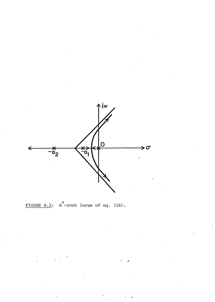
s[s(s2 + (al+a2)s + ala2) + id*] = 0 (16)

where d* is given by eqn. (10).

Again, there is a pole frozen at the origin corresponding to the eigenvector:

e = O; = e 0;

p

Now, however, the d*-root locus of eqn. (16) displays a third-order pattern as shown in Figure 4.2.

For d* large enough, i.e. large r and y* in eqn. (10), the system (15) will not only be oscillatory but also will become unstable. This holds

even when r and y* are constant and the system is in the final approach stage of adaptation. Thus, the simulation results reported in Section 2

concerning unmodeled dynamics are now explained and can even be predicted according to the preceding analysis.

4.2 The Algorithms of Narendra-Lin-Valavani [3] and Morse [4]

In order to extend the proof of asymptotic stability to the case where the relative degree of the plant is greater than one, the authors of [3] added an error feedback term so that the control input now is given by:

jiw

.10

~>0

*~

~

-02 o -0l

u(t) = l₁(t)y(t) + 82(t)r(t) - p(Ylly2(t) + (Y12+Y2 1)y(t)r(t) + Y22r (t))e(t) (18)

with an arbitrary gain p > 0.

Although this feedback term was originally incorporated in [3] to

provide technical details in the proof of stability,we shall now demonstrate that it will improve the stability characteristics of the algorithm along the lines discussed in the preceding sections for the final approach phase.

In this section we show that the extra term serves to reduce the order of the patterns of the d*-root loci both for the properly modeled system of Section 4.1.1, as well as for the system with an unmodeled pole discussed in Section 4.1.3. The added term removes the high frequency control input from the properly modeled case and allows the retention of stability when there is one unmodeled pole. However, the same high-frequency problems are still present when the reference inputs are large. In a sense they have only been shifted by one unmodeled pole, that is, there still are high

frequency control inputs when there is one unmodeled pole and, eventually, instability in the presence of two unmodeled poles.

Finally, the algorithm of Morse [4] is identical to the algorithm of [3] for the case where the relative degree is greater than one and it reduces to the algorithm of [11 and [2] when the relative degree of the plant is equal to one.

4.2.1 Analysis with Constant Inputs and Proper Modeling

With the system set-up described by eqns. (1) and a choice of control input as in eqn. (18), the error-equation now becomes

where d is as d* in eqn. (10) with y replacing y*. Equations (19), (7.c) and (7.d) now define the error system. Again, applying the final approach, i.e. by linearizing, the resulting linear system is given by

d e

1

dt

1#1/

2/I -L .Y_{2 1}Y*-Y_{2 2}r 0 0

.

with d* now given by eqn. (10)

Its characteristic polynomial is given by:

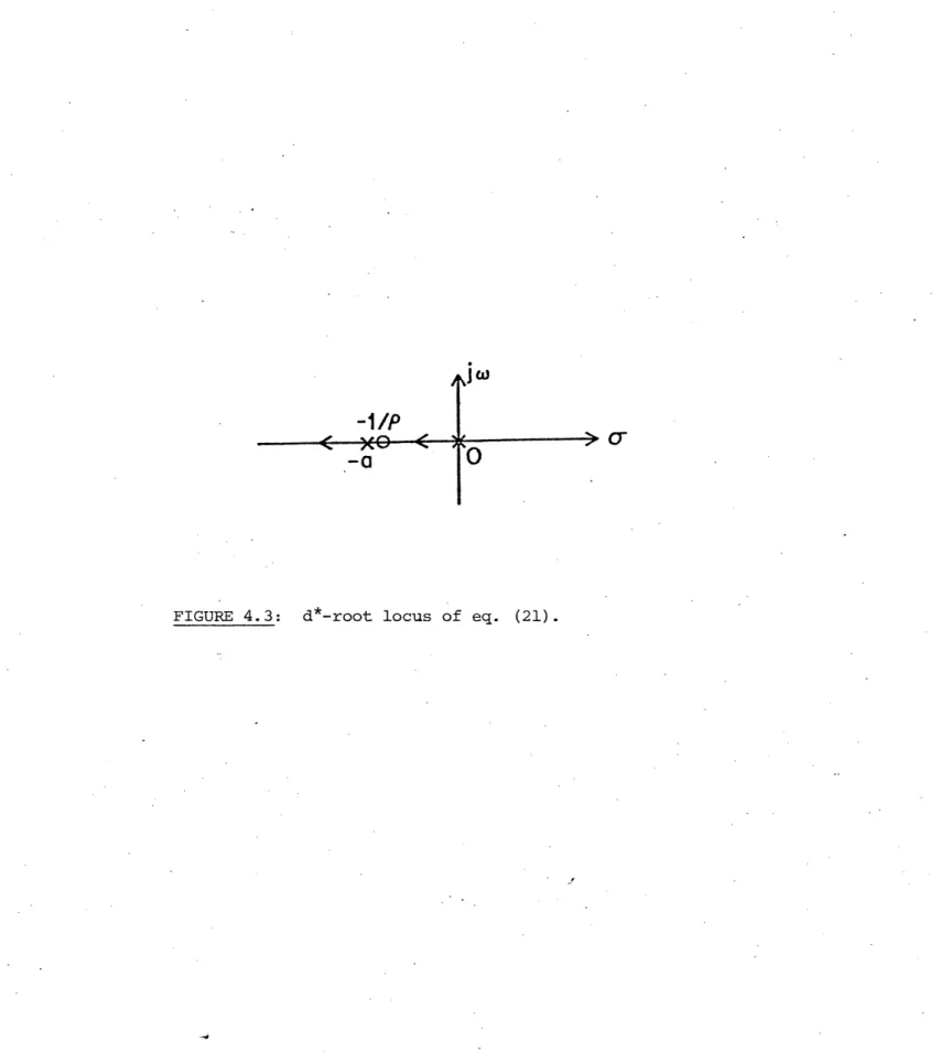
s(s + as + 6d*p(s + l/p)) = 0 (21)

Again the pole at the origin corresponds to the situation described by eqn. (11). In this algorithm, however, the d*-root locus of eqn. (21) as given by Figure 4.3 has, in addition to poles at the origin and at -a, a zero at -1/p. Since the parameter p is at the discretion of the designer, this zero may be placed to enhance the final approach stability properties as shown in Figure 4.3. The existence of the zero creates a first-order pattern so that there are no high frequency oscillatory control inputs. 4.2.2 Analysis with Constant Input and Unmodeled Dynamics

If there is an unmodeled pole in the plant the same analysis as in Section 4.1.3 shows that there is again a pole at the origin and a d*-root locus as in Figure 4.4 which results from the characteristic equation

s[s(s2 + (al+a2)s + ala2) + gd*p(s+l/p)] = 0 (22)

The system remains stable for all values of d* although the second order pattern shows that there will be high frequency control inputs for large

-1/P '>

-aFIGURE

4.3:

locus of eq. (21)

droot

-1/p

02

_l

values of d*.

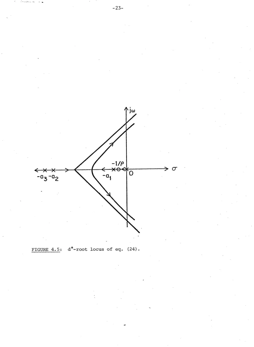
If it is assumed that there are two high frequency unmodeled poles at -a2 and -a₃ and there also exists a stable third order model

'+ p* P2 + pY * + p PoY* = b3r (23)

with P2 = al + a2 + a3 and P1 = a1l 2 + aLa3 + a2a3 such that the d.c. gain

at eqn. (23) matches that of eqn. (l.b), the resulting system has the char-acteristic equation

s[s(s5 + p2s + p1s p + o) + id* (s + l/p)] (24)

As shown in Figure 4.5, the d*-root locus has a third order pattern and instability will result for large values of d*.

4.3 An Improvement in Final Approach Behavior for Constant Reference Inputs Although the added feedback term of the algorithm of Section 4.2 improves the final approach behavior, the problem still remains that large reference inputs cause the adaptive system to try to react too quickly, thus generat-ing high frequency control inputs, as in the case of one unmodeled pole in the preceding section. In this section it is shown that, if the adaptive gains can be used to artificially slow down the adaptation process when the reference inputs are large, a smaller bandwidth system and improved final approach behavior will result.

In order to achieve this the adaptive gains must be functions of the reference input. However, global asymptotic stability has only been proven for the case of constant adaptive gains or certain restricted types of time varying gains. Thus, the approach that follows is only theoretically valid for the case of constant reference inputs, a case of considerable practical

jw

G/

-03 -02

t

significance for cases where the control system is to be designed to follow set-point changes,where the reference input is constant for long periods of time. In addition, the insights gained by examining this approach will add to our ability to analyze discrete-time systems where more flexible stability proofs exist.

The modification in the adaptive gains may be applied either to the algorithm of Section 4.1 or to that of Section 4.2 with equivalent results, For simplicity, the former will be used.

The algorithm of interest here is identical to that of Section 4.2 with one exception; that the constant matrix of adaptive gains

-old

(25)

L 21 ¥22

is replaced by the following one

1

r

-new 2 2 -old

y+r +y*

The analysis of Section 4.2 also goes through exactly with the exception that eqn. (10) is now replaced by

y* T rY*1

d* = ew r (27)

with the condition 22 y*2+r

2 2 maxf old < ma (old) (28) Y+y* +r

where max (o ld) is the maximum eigenvalue of rold ad y > 0. Both omax(rold) and y are under the designer's control.

Thus given an upper bound on , max (rold ) can be chosen to limit how far along the d*-root locus of Figure 4.1 or the d*-root locus of Figure 4.2 the roots of the system can travel. Consequently, the maximum frequency of parameter error variation in the final approach is under the direct con-trol of the designer. Also, with an upper bound on d*, the adaptive system is able to handle any number of high frequency unmodeled poles while retain-ing local final approach stability.

The parameter y is used to control the value of d* when y* + r is small. Note that from Figures 4.1 and 4.2 the error system is sluggish for small values of d*. If y is set equal to the smallest value of y* + r expected, the result is d* > 2 and the area in which the error system poles will lie may be controlled. The reader is reminded, however, that if r and y are too small, the final approach analysis presented here may not be valid.

5. FINAL APPROACH ANALYSIS OF SOME DISCRETE TIME ALGORITHMS

In this section, some of the discrete time adaptive control algorithms that have been presented in the literature are subjected to the same final approach analysis as in the continuous-time case. The discrete time setting has allowed for somewhat more flexible control algorithms that are

theoretical-ly globaltheoretical-ly asymptoticaltheoretical-ly stable. In the present section we show precisely what is good about this added flexibility and how it may be utilized in a practical context. It should be noted here that such flexibility resulted

as a byproduct of the different methods of proving stability that are in existence for the discrete-time problem. This paper provides the first attempt to use this flexibility in order to achieve more desirable system characteristics.

5.1 Analysis of the Algorithm of Narendra-Lin [5]

The algorithm of [5] is the discrete time analog of the algorithm of Section 4.2. However, the stability improving extra feedback term of Section 4.2 which was not always necessary for the global stability proof in the continuous time case, is necessary in the discrete-time case, i.e. the direct discrete-time analog of the algorithm of Section 4.1 is not globally asymptotically stable. In this section it will be seen how the extra term provides for improved stability characteristics in the final approach phase.

The set-up is as in eqn. (2). The input is generated Analogously to eqn. (18), i e.

u(t+l) = e1Ct+l)y(t) + O2(t+l)rCt+l) - P(Y1 1y 2(t) + (y1 2+YZ2 )Y(t)r(t+l) +

2

2

2tl)et

(29)

-p(ylly(t + ( 1 2+Y21 )Y(t)r(t+l) + Y22r (tl))e(t+l)] (29)

with all quantities defined as in the continuous time case and - < p < 1.

The error equation for this system is:

e(t) = y(t) - y*(t)

ae(t-l) + l(t)y(t-l) + 2(t)r(t) (30.a) 1 + pfd (t) where 2 2 d (t) Y y Y2 (t-i) + (Y1 21 +Y2 )y(t-r(t) + r (t) (31)

The adaptation equations in complete analogy to eqns. (7.c) and (7.d) are:

l(t+l) l(t)

-₁ l f -f Y y(t-l)e(t) - y 2r(t)e(t) (30.b)

c2(t+l = 2(t)

= B - y_{2 1}y(t-l)e(t) - Y2 2r(t)e(t) (30.c)

5.1.1 Analysis with a Properly Modeled System

With a state vector consisting of e(t-l), 1l(t) and p2(t), substitution

of eqn. (30.a) in eqns. (30.b) and (30.c) and subsequent application of the

e (t)

a

l+pSd* l+pSd* - l+pSd*

Yl(t+l) 2

-Y¥lay*-y_{1 2}ar (-Y1 1llY* 12 - 1 -2Y*r) y*r-YY22 2r

B 1 + 2+p(d* l+p(d* l+pfd* 22 (t+l)

L

with y* = y*(t-l), r = r(t) and d* as defined by eqn. (31) with y* replacing y. This system (32) has the characteristic equation:

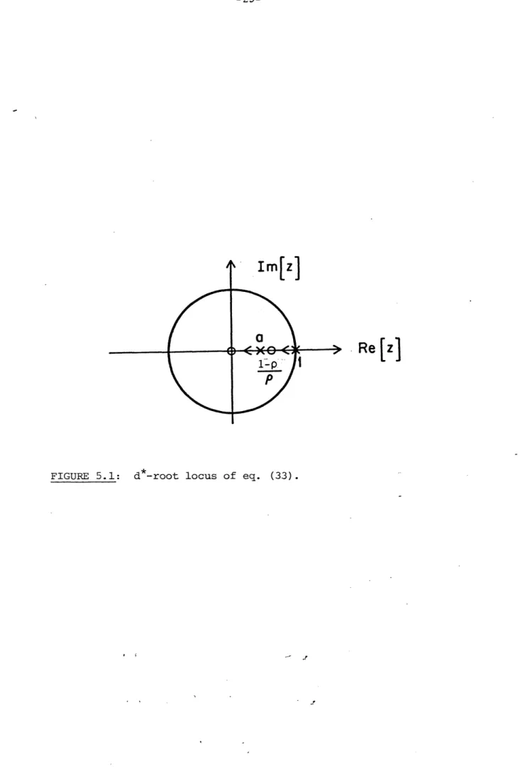
(z-l)[(z-l)(z-a) + + P- )] = 0 pd*P(z(z (33)

There is a marginally stable pole frozen at z=l associated with the eigenvector

e(t-1) = 0; ¢₂(t) = r(t) (t) (34)

Two other poles appear in a d*-root locus as shown in Figure 5.1. One pole starts at z=a and the other at z=l and, with increasing d*, move towards the zeros at z=O and z = p . The latter zero is, however, determined by the designer by use of the parameter P.

If the added feedback term of this algorithm were not present, the 1-p

zero at z = p would be missing. As a result, one of the poles would move along the negative real axis towards infinity causing a chatter type instability, characteristic of discrete-time systems.

~

Iw)[z]

;,

,

Re[z

5.1.2 Analysis with an Unmodeled Pole

The set-up of eqn. (4) is used with the assumptions given there. The system is constructed by using eqns. (29), (30.b) and (30.c) as if there were only one pole. The output error equations then become

(al+a2)e(t-l) - ala2 e(t-2) + ~l(t)y(t-l)+ ~2(t)r(t)

e(t) = (35)

1 + pCd (t)

The final approach analysis yields the following characteristic equation:

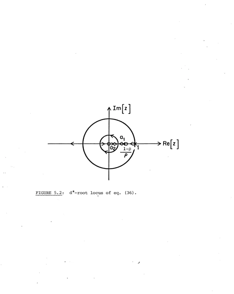
(z-l)[(z-l)(z - (al+a2)z + ala2) + Ed* (z(z + l))] = 0 (36)

The d*-root locus of Figure 5.2 shows that the error system will become unstable for large reference inputs.

The same choice of adaptive gains can be made here as was made for the continuous algorithm in Section 4.3 to produce the same desirable final approach characteristics. However, as in the continuous case, the stability proof is valid only for constant gains, as discussed before.

5.2 Analysis and Suggestions for Landau's and Silveira's Algorithm [6],[7] In [6] and [7] stability theorems were given which used Popov's

hypestability theory to effectively generalize the algorithm presented in Section 5.1 in order to include certain types of time-varying adaptive gains. In this section it will be shown that, if the free parameters of the algo-rithm of [7] are chosen properly, the bandlimiting effect and improved final approach behavior of Section 4.3 can be achieved for slowly varying reference inputs while global asymptotic stability is also retained.

, rm-Re[z]

FIGURE 5.2: d*-root locus of eq. (36).

by eqn. (29) and the parameter updates by eqn. (30). In addition, we define

[¥11) Y )(t)

-'(t) =.l

2

Jand

- (t) Y r(t)

and add to the aforementioned set of equations the following adaptive gain adjustment equation:

r

F(t+l) = r(t) X T.T (38)

I~·,1 -I + k2w T ( t)r ( t) w ( t ) Also, we set p = 1 for convenience.

Let H(z) be the model transfer function and let X be the largest value such that

H(z) - - is strictly positive real (39)

Using the model of eqn. (2.b) the condition for stability is that

bz k

bza X is strictly positive real (40)

For C(0) > 0, 0 <

x1

The adaptive gain adjustment described in eqn. (38) is motivated by the use of the matrix inverstion lemma which shows that when r(t) and r(t+l) are

invertible,

r-l(t+l)

The final approach analysis of Section 5.2 holds here as well. In particular, the characterisic equation of the error system is now given by

eqn. (33) with p=l

(z-l)[(z-l)(z-a) + Bd*z2] = O (42)

with d* given by

d* = w*Trw * (43)

The d*-root locus of eqn. (42) is drawn in Figure 5.3

If r is constant and eqn. (41) is in the steady state, eqns. (41) and (43) yield

1-1

d* = (44)

2

With an upper bound on X, the gain on the root locus of Figure 5.3 can be bounded, thus limiting high frequency behavior and retaining stability

in the presence of unmodeled poles.

In general, the problem is to keep d* small so we let X2 = min(X,2). The choice of X1 is then a trade-off between keeping the value of d* low in

the steady state and making the dynamics of eqn. (41) fast enough so that the steady state analysis is valid. For problems where an appropriate com-promise can be achieved, the improved final approach characteristics can be

attained without sacrificing the global stability analysis.

5.3 Analysis of the Algorithm of Goodwin, Ramadge and Caines [8]

The algorithm in [8] uses a different philosophy than the previous

Im[ z

( \ t

t-~>

Re[z]

FIGU-RE 5.3: d -root locus of eq. (42).

with the controlled plant and try to make the controlled plant identical to

the model, the algorithm in [8] uses a serial combination, as in Figure 5.4

where the model predicts the desired output. The algorithm then tries to

transform the controlled plant into a pure time delay.

In the present section, it will be demonstrated that such a deadbeat

control scheme removes the dynamics of the output error from the overall

adaptive system. This makes possible the stability proof of [8] with

time-varying adaptive gains of the type discussed elsewhere in this

paper--gains which limit the bandwidth of the parameter-error system. There is,

however, a serious drawback; the high gain requirements of the deadbeat

con-trol scheme make the adaptive system susceptible to instability due to

un-modeled dynamics. This is consistent with the remarks of Section 3 although

it is better shown graphically by a different analysis which we shall employ

in this section.

We note that although there are three algorithms presented in [8] they

are all qualitatively the same and, therefore, only the second will be

analyzed here.

5.3.1 Analysis with Proper Modeling

The system used for this analysis is:

y*(t+l) = ay*(t) + br(t) (45.a)

y(t+l) = B(a'y(t) + u(t)) (45.b)

where a' corresponds to ~ in eqn. (2). The algorithm estimates a' as a'

1 and generates the control as follows:

r( k) Mdel y (k+r)Cotrole

F E

1 A

u(t) = t) yy*t+l) (t) (46)

The identification and implicit control scheme then forms the error as in eqn. (6)--which in this case corresponds to the input error of the

identification literature--, and updates the parameters by the algorithm

1 y(t)e(t+l) at(t+l) = a (t) + (t) 2 (47.a) 1 + y (t) + y* (t+l) A A A I I y(t+l)1(t+l) 1(t+l) (t) -1 (t) t+l)et+l) (47.b) 1 + y2 (t) + *2 (t+l)

Letting 1(t) = ( a' - '(t) and p2(t) =

i

1

e(t+l) = l(t)(t) + 2(t)y*(t+l) (48)

and is free of any dynamics. Using eqn. (48) in eqn. (47) and applying the final approach analysis we obtain:

[l(t+l)] [1 + y*2 (t+l) y* (t)y*(t+l)] [l(t)] P (t+l) y*(t)y*(t+l) 1 + y*2 (t)

J

with

d*(t) =2 2 (50)

1 + y* (t) + y* (t+l)

When y* is constant, the system (49) has the characteristic equation

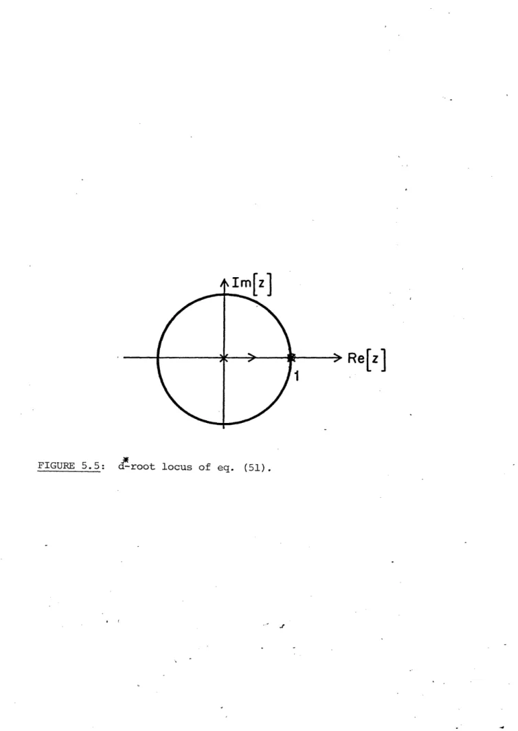
Two facts about d* are needed to properly interpret the d*-root locus of eqn. (51) shown in Figure 5.5:

1. d* decreases with increasing r and y*. This is the inverse relationship from that in the previous algorithms.

2. 0 < d* < 1. It is this fact that stops the movement of the pole in Figure 5.5 at z=l and retains stability.

Despite the differences in philosophy, both the algorithms of this section and that of Section 5.1 can be seen to originate from a discrete-time version of the algorithm of Section 4.1. That algorithm cannot guarantee stability because large inputs would cause a pole of the error system to move out of the unit circle in a first order pattern in the d*-root locus. In the algorithm of Section 5.1 this problem was solved using an added feedback term to create a minimum phase zero in order to trap the otherwise wandering pole. The algorithm of this section uses an adaptive gain d*(t) given by eqn. (50) which limits the range within which the poles can travel, similar to what was seen in Section 4.3. However, in order to prove stability in this case, a restriction that the controlled plant be a dead-beat system must be placed on the system.

Thus, the two adaptive control systems are indeed similar. In fact if the extra feedback term of eqn. (29) is removed (p=O), the model of that system is taken as a pure time delay (a=O) and the adaptive gains are chosen by yii = + y 2 2 v the two systems are indeed equivalent.

1 + y (t) + r (t+l)

5.3.2 Analysis with an Unmodeled Pole

Im~z)

Re[z]

y(t+2) = (ai+ 2)y(t+l) - alla2Y(t) + Bu(t)

= SJjt - y(t+l) - y(t) + u(t) (52)

The adaptive controller is the same as if there were only one pole so

^

1

eqn. (47) still holds although a and ~ are now merely symbols of parameters, since they have lost their meaning in terms of what they represent in the

plant. A slightly different analysis from the one used in previous sections

is employed here. Assume that y* is constant so that

e(t+2) = y(t+2) - y*(t+2) = y(t+2) - y*(t+l)

F1+

y

*

t

= {I zl 2 y(t+l) - - t+l)- 2 + (t) Y(t) ('s3)

2

i a 1+a2 1

Set

4l(t)

ov(t)

e(t+2) = [l 2 e(t+l) - (l(t)y(t) + P2(t)y*(t+l)] (54)

so that

e(t+l) = 0, tl( = 0, Pt) = 0 , e2(t+2) = 0 (55)

The final approach analysis then yields

e(t+2) 1 + 2 -y*(t) [y*(t+l) e(t+l) d*(t)y*(t)

d1l(t+l) d(1 0 Pl(t) (56)

with d*(t) defined by eqn. (50).

The characteristic equation of (56) is:

(z-l)(z -(a₁+a ₂+l)z + (al+a₂+l)-d*) = 0 (57)

According to the present analysis, the dependence of the error model upon

the unknown plant is shown directly as opposed to the discussion in Section

3. The magnitude of one of the poles must be greater than or equal to

l+al+a2

2 . Therefore, the error system cannot be stable if the plant poles

are on the positive real axis and the plant is unstable. This was

predicted in Section 3 to be a result of the dead-beat philosophy. Indeed,

even if the plant is stable, a large enough input will make d* small enough

so as to finally make the resulting error system unstable.

In order to understand the basic problem with using a dead-beat

con-troller when there are unmodeled poles, we consider the problem of

creat-ing a dead-beat controller even when the parameters of the plant are known.

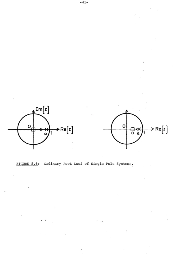
Figure 5.6(a) displays the ordinary feedback gain root locus in the case

where a plant with a pole at a is connected in feedback with a scalar gain. In order to achieve dead-beat control, the gain must be large enough to

push the pole to the origin; in this case the gain must equal a. This is

a much larger gain, than is normally required to meet the objectives of a

typical parallel structure adaptive controller, as shown in Figure 5.6(b),

i.e. to drive the pole to point a, the pole position of the model. This only

requires a gain of a-a.

If there is a high frequency unmodeled pole, the dead-beat controller cannot come close to meeting its objective and the high gain used in

X

Re[z]

Re[1

attempting to do so may drive the system unstable as shown in Figure 5.7(a). On the other hand, the parallel system may be little affected if the pole is of high enough frequency as in Figure 5.7(b).

Thus, while the dead-beat algorithm [8] allows for improved final approach characteristics when the system is properly modeled, it inherently has poor robustness properties in the presence of unmodeled dynamics.

Im

z]

Im[z]

/

₀₁

_Rez

_O

FIGURE

7:

Ordinary

Root Loci of Systems with One U odeed Pole

FIGURE 5.7: Ordinary Root Loci of Systems with One Unmodeled Pole.

.~~~~~~~~~~~~~~~~~~~~~~~~~~~-6. AN EXPLANATION OF THE--UNDESIRABLE EFFECTS OF OUTPUT NOISE

It was noted in Section 2 that observation noise added to the output y resulted in a closed loop system of an increasingly wider bandwidth. This phenomenon was observed in simulations, carried out on the digital computer, of a discretized version of the algorithm of Section 4.1, to which discrete-time white noise was added.

In this section, the discretized version of the algorithm in Section 4.1 is obtained and its equivalence with the continuous-time system is shown with respect to characteristics displayed when final approach analysis is employed. Subsequently, the effect of observation noise is examined and the analytical results corroborate the simulation findings mentioned in Section 2.

6.1 The Discretized Version of the Algorithm of Section 4.1

For the simulations discussed in Section 2, the continuous-time algorithm was sampled at a high rate, with the resulting discrete system described by the following set of equations:

-aT ₁ eaT 1-e-aT

e(t+l) = e e(t) + a Y1(t)y(t) + - 2ea 2(t)r(t) (58a)

1(t)

pl(t+l) = 8 -. Ty(t)e(t) (58b)

(2(t)

where T is the sampling period. The adaptive gains were chosen as 11 22 12 = Y21 =0 in the simulation.

The characteristic equation of system (58) via the final approach analysis is obtained as (z-l) [(z-l)(z-ad)+ d*]=0 (59) where ad = exp(-aT) -aT l-e a and d gT(y +r ) (60)

Since T is very small and g T as a consequence, the

d*-root locus of eqn. (58) as given in Fig. 6.1 has the same charac-teristics as its continuous-time counterpart, as is seen from Fig. 4.1.

6.2 Analysis with Output Noise

When observation noise, n(t), is present at the output of the plant, eqn. (58) becomes

e(t+l) = ade(t) + gl(t)(y(tnt)+n(t) + gc2(t)r(t) (61a)

$i(t+l) S(lt)

1= 1 - T(y(t)+n(t))(e(t)-n(t)) (61b)

~2(t+l) ¢2(t)

Re[z]

which, when subjected to the final approach analysis with the assumption of a constant reference input, yields the following system:

e(t+l) ad ag (y*+n(t)) Bgr e(t)

41(t+l) _ -T(y*+n(t)) 1 0 (t) -Tr 0 1

¢2

(t+l)

2(t)

A first point to notice here is that this discretized algorithm is not guaranteed to be globally asymptotically stable in the presence of observation noise. Large values of the noise n(t), at any time t, will cause the system matrix, in eqn. (62) at that time to be unstable;

i.e. its eigenvalues will not all lie within the unit circle. In order to avoid this effect we assume that the noise is bounded and that the sampling periodT is chosen small enough so that the system matrix at every time remains stable. We also assume that n(t) has a zero mean and a constant variance, a , at each time, and that all time samples are independent.

The characteristic equation of the system matrix in eqn. (62) is given by eqn. (63) following:

A(z) = (z-l)[(z-l)(z-ad) + d*(n(t))]=O (63) where

d*(n(t)) = gTB[(y*+n(t)) 2+r2] (64)

Thus the system always contains a marginally stable pole located at z=l. Associated with the pole is a time-varying eigenvector whose components are described by eqn. (65):

e=O c1 = -r ~2 = y*+n(t) (65)

We assume that the constant input r is not equal to zero, so that the remaining two poles of the system are associated with asymptotically stable modes.

In what follows, we first examine the effect of the n (t) driving term in eqn. (62). This term arises because in the parameter updating law the error at time t is multiplied by the plant output at the same time and they are both corrupted by the additive noise n(t) at that instant of time. The individual transfer functions from the n2(t) driving term to the output and parameter errors are given by eqn. (66)

-T~g(y*+n(t))(z-l) A(z) h 2 (z) = T[(z-ad) (z-l)+ gTr2] (66) n (t) A(z) T fg r(y*+n(t)) A(z) has been (6defined in eqn. where A(z) has been defined in eqn. (63).

We note that in the transfer function from the n2 (t) term to the output error the marginally stable pole at z=l is cancelled by a zero. Thus the n (t) term, with constant variance 2?, will cause only a bounded and relatively small output error bias. The marginally stable pole at z=l is however present in the transfer functions from the n (t) term to the parameter errors. If the eigenvector associated with this pole were time invariant, the non-zero mean of n (t) would drive these parameter errors to infinity. We conjecture that the movement of the eigenvector with time makes the transfer functions from the n (t) term to the parameter errors asymptotically stable although possibly with a large gain. This conjecture is supported by the intuitive explanation of the effects of time-varying eigenvectors on parameter convergence,

given in Section 4.1.2 and by the proof contained in the following section, which shows that indeed such a phenomenon does occur in a similar

algorithm. Thus, the parameter errors would increase and then level off. The preceding observation gives an analytical explanation for the sim-ulation results of Section 2 where the output error remained bounded while the increasing parameter errors resulted in an ever-increasing bandwidth system.

If the noise statistics were known, the effect of the non-zero mean of n (t) could be removed from the error equations by merely subtracting the term To2 from the update algorithm of the first parameter, i.e.

eqns. (58b) or (61b). If the conjecture discussed above, namely that the time-varying nature of the eigenvector associated with the marginally

stable pole eventually brings about asymptotic stability of the transfer

functions for all error components holds, the result would be a zero bias

and bounded variance system due to the n (t) driving term.

As far as the effect of the n(t) driving term is concerned, it is

similar to the effect of an (n2 (t)-o2 ) term except that, in this case, the

system is completely controllable from the linear noise term. Therefore,

the marginally stable pole is not cancelled in the path from n(t) to

e(t).

In more precise terms then, the conjecture states that, if To2 is

subtracted out of the algorithm as suggested above, the result would

be a mean-square bounded error system although the error variance may be

large compared to the noise variance. This can be explained by the

fact that the error variance is also determined by the rate of convergence

that the particular observation noise induces on the overall algorithm.

In the following section, we prove boundedness of the associated

output and parameter errors, in a mean square sense, for a similar algorithm

to that described by eqn. (61). The proof is independent of any boundedness

assumptions on the noise and is carried out for the original nonlinear system

of difference equations and not for the linearized final approach system that can be derived from them.

7. MEAN-SQUARE BOUNDEDNESS OF THE NARENDRA-LIN r5] ALGORITHM IN THE PRESENCE OF WHITE GAUSSIAN OBSERVATION NOISE

In the present section we prove that for a first order plant, the output and parameter errors of the algorithm in [5] (section 5.1 in this paper) remain bounded in a mean-square sense when the plant output

is corrupted by a measurement noise sequence assumed to be white, Gaussian of zero mean and arbitrary constant variance. The proof makes use of the ideas of Bitmead and Anderson, [12],[13], and Anderson and Johnson

[14]. In addition, an expression for a bound on the weighted mean-square error is derived.

We believe that this is the first proof that an adaptive control algorithm with observation noise is mean-square stable not only in the output but in the parameter errors as well, independent of the choice of

a reference input. This confirms the often expressed belief that the output noise will infact provide the "sufficient excitation" necessary for parameter error boundedness at least in the case considered here.

Next, we proceed with the algorithm of section 5.1, where we set p=l and

r=

We then assume that a noise sample n(t) is added to the observations of y(t) at each instant t. The resulting error system is now described by the following set of equations:

e(t) 1 z e(t-1)(t-l) efa 1 Bzl(t) 1r(t) ~1 (t+l)

12(t)

Y2ar(t) -By2z(t-l)r(t) 1+Sd(t)-y2 Br2 (t)

J

SB

$d(t)

l+Sd(t) ylz(t-l) n(t) (67)

y2r(t)

where all quantities are defined analogously as in section 5.1, with d(t) given by

d(t) = YlZ (t-l) + 2r 2(t) (68)

where z(t) is a noise corrupted signal

z(t) = y(t) + n(t) . (69)

and {n(t), t=O,...,o} a zero-mean white noise sequence with each sample having variance a .

Note that, in this algorithm, the error at time t is multiplied by the noise corrupted plant output at time (t-l) for the parameter

adjustment laws. Since the additive noise samples at those two times are assumed to be uncorrelated, the expected value of the noise driving term in eqn. (67) is zero. Equations (67) can alternately be

written as follows:

x(t+l) = A(t)x(t) + B(t)n(t) (70)

where the correspondence of A(t), B(t), and x(t) with the elements of

eqn. (67) is self-evident.

The weighted mean square error for a particular time t can now

be written as E[x'(t)Px(t)] where P=pT>0.

Similarly, at time 2(t+l) the corresponding error- before taking expected

values- is expressed as

x'[2(t+l)]Px[2(t+l)] . (71)

Substitution of eqn. (70) in expression (71), in turn, yields:

x'(2(t+l))Px(2(t+l)) = x'(2t)A'(2t)A'(2t+l)PA(2t+l)A(2t)x(2t) +

+ 2x' (2t)A' (2t)A' (2t+1)PA(2t+l)B(2t)n(2t)+2x(2t)A' (2t)A' (2t+l)PB(2t+l)n(2t+l)+

+ n(2t)B'(2t)A'(2t+l)PA(2t+l)B(2t)n(2t)+2n(2t)B'(2t)A'(2t+l)PB(2t+l)n(2t+l)+

+ n(2t+l)B' (2t+l)PB(2t+l)n(2t+l) (72)

Subtracting the term x'(2t)A' (2t)PA(2t)x(2t) from both sides of the

+

+ 2E[x' (2t)A' (2t)A' (2t+l)PA(2t+l)B(2t)n(2t)] +E[n(2t)B' (2t)A' (2t+l)PA(2t+l)B(2t)n(2t)]

+ E[n(2t+l)B' (2t+l)PB(2t+l)n(2t+)] _{. (73)}

Straightforward algebraic manipulations for the algorithm of eqn. (67) shows in turn, that the following equality holds for all t.

A' (t)PA(t)-P = -H(t)H' (t) (74) where 1/ o o0 p = O 1/Y1 0 ₍₇₅₎ 0 0 1/ 2 (l+pd(t)) afd (t) d-(t)a and H(t) _{1+and d(t) H(t) 0 - z(t-l) Vd't)z(t-l)} 0 -V

r

r

Finally, substitution of eqn. (74) in the first term on the RHS of eqn. (72) allows it to be rewritten as

-E[x'(2t){A'(2t)H(2t+l)H'(2t+l)A(2t) ₊ H(2t)H'(2t)}x(2t)] =

where

W(2t) {A'm(2t)H(2t+l)H'(2t+l)A(2t) + H(2t)H'(2t)}

In what follows we prove next that W(2t)> P(2t)P where p(2t)>O for

all t within two consecutive time steps.

Let W(2t) - L(2t)L'(2t) (78) where L(2t) = [H(2t) A' (2t)H(2t+l)] (79)

0O

oEy(2t)

where X (TT') is the maximun eigenvalue of TT'. Direct calculation

max

shows that

Further, it can be straightforwardly shown that

W '1Y2 (gz(2t)r(2t)- z(2t-1)r(2t+))2 P (85) -W(2t) 2 (l+Bd(2t)) (1+d(2t+l))

with P given by (75) since

l+d(2t)-a' + a (l+6d(2t+l)-a') 0 0 8(l+Sd(2t)) (1l+d(2t+l)) W(2t) = O 2(2t-1) z2(2t) + 8z(2t-1)r(2t) Bz(2t)r(2t+l) l+Bd(2t) l+Bd(2t+l) l+Bd(2t) l+z d(2t+l) 0O 8z(2t-l)r(2t) + Bz(2t)r(2t+l) Br2(2t) + Br2(2t+1) l+ad(2t) l+Bd(2t+l) l+$d(2t) l+Bd(2t+l)

Combining eqns. (83), (84) and (85) yields that

W(2t)> p(2t)P (86)

¥1Y2 (Sz(2t)r(2t)- z(2t-l)r(2t+l))2

where ip(2t) - (1+Y1+Y2.\ l+Bd(2t))(l+Wd(2t+l)) (87) 2max 1Y 12,

)

We note that p>O unless

{y(2t)+n(2t)}r(2t) = {y(2t-l)+n(2t-l)}r(2t+l) (88) an event which occurs with zero probability. Also

E[x'(2t)W(2t)x(2t)]> E[p(2t)x'(2t)Px(2t)]

and clearly E[p(2t)]> 0 · (90) Substitution of eqns. (77) and (89) in eqn. (72) results in the

following inequality:

E[x' (2(t+l)Px(2(t+l))]<(1-E[p(2t)])E[x' (2t(Px(2t)] +

+ 2E[x' (2t)A(2t)(2t)n(2t)]+E[x (2t)A'(2t)A'(2t+l)PA(2t+l)B(2t)n(2t)]+

+ E[n' (2t+l)B'(2t+l)PB(2t+l)n(2t+1)] (91)

Next, using eqn. (74) we prove below that the second term on the RHS of ineq. (91) is less than or equal to zero, independently of the fact that A(2t+l) depends on n(2t).

Let D=E[x'(2t)A'(2t)A'(2t+l)PA(2t+l)B(2t)n(2t)]

< E[x'(2t)A(2t)PB(2t)n(2t)A(2t)PB(2t)n(2t)]=E[x' (2t)A(2t)PB(2t)]E[n(2t)]=0 (92)

Similarly, for the third term on the RHS of the same inequality, (91), it can be shown that

E[n(2t)B' (2t)A' (2t+l)PA(2t+l)B(2t)n(2t)]

< E[n'(2t)B'(2t)PB(2t)n(2t)] (93)

and, substituting the values for B and P from eqns. (67) and (75) we further get

E[n' (2t)B' (2t)PB(2t)n(2t)]

Bd2 (2t)+y1z (2t-l)+y2r (2t) i

=

E

) 1-~(

j2

E2n

=

{l+8d(2t)}

2

Ed(2t)(l+Bd(2t)) 1 En o2(2t)~ 2

In an exactly analogous manner it can be shown that

E[n' (2t+l)B'(2t+l)PB(2t+l)n(2t+l)]< c2 (95)

Combining equations (92), (94) and (95), eqn. (91) becomes:

E[x'(2(t+l))Px(2(t+l))]<(l-E[p(2t)])E[x'(2t)PX(2t)] + 2

+ D

(96)

where D<O from eqn. (92).

Equation (96) states that indeed the system (67) is mean square

stable in both output and parameter errors. Moreover, the steady

state mean square error is bounded above by

lim E[x'(2t)Px(2t)]< 2a2 (97)

t-+co __

lim inf E[ J(2t)]

8. CONCLUSIONS

A new method, called final approach analysis, has been developed to analyze the dynamic properties of a class of direct adaptive control algo-rithms[l]-[8] with special emphasis on the robustness of these algorithms to

(a) generation of high frequencies in the plant control signal

(b) excessive bandwidth of the adaptive control loop resulting in excitation of unmodeled dynamics and, consequently, leading to dynamic instability of the closed-loop adaptive system

(c) noise corrupted measurements.

An adaptive control algorithm must have reasonable tolerance to such model-ing error and stochastic uncertainties before it can be used routinely in practical applications.

With the exception of the algorithm of Landau and Silveira [6], [7], discussed in Section 5.2 for the deterministic case, the final approach analysis has shown that all other algorithms studied have unacceptable dynamic characteristics. Thus the analytical results confirm the authors' simulation experience described in [9].

The final approach analysis is useful because it can be used in a con-structive way to adjust the adaptive gains so as to limit the closed-loop system bandwidth and to ameliorate some of the undesirable characteristics of existing adaptive algorithms. Additional research is underway to extend the ideas presented in this paper to high-order systems,

We believe that the final approach analysis is a necessary but by no means sufficient step in the analysis and design of adaptive systems. The

technique is limited to the cases in which the output error is small and

does not change rapidly so that dynamic linearization of the complex

non-linear differential or difference equations that describe the adaptation

process [1]-[8] makes sense. By itself, it cannot predict what happens in

the truly transient phase; the simulation results presented in [9] suggest

that even more complex and undesirable dynamic effects are present.

The paper also contains a proof- the first to appear in the

literature-of the mean square boundedness literature-of the parameter errors in addition to the same

for the output errors previously obtained, for one of the discrete-time

algorithms analyzed here in the presence of observation noise. The proof

was obtained for the original system of nonlinear difference equations and

although it applies to a scalar plant in the present paper, it is

extendable to the multivariable case as well.

It is our opinion that a great deal of additional basic research is

needed in the area of adaptive control. Future theoretical investigation

must, however, take drastically new directions than those reported in the

recent literature. The existence of unmodeled dynamics and stochastic

effects must be an integral part of the theoretical problem formulation.

In addition, future adaptive algorithms must be able to deal with problems

in which partial knowledge of the system dynamics is available (see the

discussion at the end of Section 1) so that at the very least the

inten-tional augmentation of the controlled plant dynamics with roll-off and

noise rejection transfer functions can be handled without confusing the

shaping in the frequency domain) is necessary even in non-adaptive modern control systems [15] for good performance and stability;

clearly the same techniques must be used in adaptive systems. The algorithms considered in the paper cannot handle the additional dynamics because

the existence of the latter violates the theoretical assumptions necessary to assure global stability.

REFERENCES

[1] K.S. Narendra and L.S. Valavani, "Stable Adaptive Controller Design-Direct Control", IEEE Trans. Automat. Contr., Vol. AC-23, pp. 570-583, Aug. 1978.

[2] A. Feuer and S. Morse, "Adaptive Control of Single-Input Single-Output Linear Systems", IEEE Trans. Automat. Contr., Vol. AC-23, pp. 557-570, Aug. 1978.

[3] K.S. Narendra, Y.H. Lin and L.S. Valavani, "Stable Adaptive Controller Design, Part II: Proof of Stability", IEEE Trans. Automat. Contr., Vol. AC-25, pp. 440-448, June 1980.

[4] A.S. Morse, "Global Stability of Parameter Adaptive Control Systems", IEEE Trans. Automat. Contr., Vol. AC-25, pp. 433-440, June 1980.

[5] K.S. Narendra and Y.H. Lin, "Stable Discrete Adaptive Control", IEEE Trans. Automat. Contr., Vol. AC-25, pp. 456-461, June 1980.

[6] I.D. Landau and H.M. Silveira, "A Stability Theorem with Applications to Adaptive Control", IEEE Trans. Automat. Contr., Vol. AC-24, pp. 305-312, April 1979.

[7] I.D. Landau, "An Extension of a Stability Theorem Applicable to Adaptive Control", IEEE Trans. Automat. Contr., Vol. AC-25, pp. 814-817, Aug. 1980. [8] G.C. Goodwin, P.J. Ramadge and P.E. Caines, "Discrete Time Multivariable

Adaptive Control", IEEE Trans. Automat. Contr., Vol. AC-25, June 1980. [9] C. Rohrs, L. Valavani and M. Athans, "Convergence Studies of Adaptive

Control Algorithms, Part I: Analysis", in Proc. IEEE CDC Conf., Albuquerque, New Mexico, 1980, pp. 1138-1141.

[10] H. Elliott and W.A. Wolovich, "Parameter Adaptive Identification and Control", IEEE Trans. Automat. Contr., Vol. AC-24, pp. 592-599, Aug.

1979.

[11] G. Kreisselmeier, "Adaptive Control Via Adaptive Observation and Asymptotic Feedback Martic Synthesis", IEEE Trans. Automat. Contr., Vol. AC-25, Aug. 1980.