Applications of machine learning : basketball strategy

Applications of Machine Learning: Basketball Strategy

by

Santhosh Narayan

B.S. Computer Science, Massachusetts Institute of Technology (2015)

Submitted to the Department of Electrical Engineering and Computer Science

In partial fulfillment of the requirements for the degree of

Master of Engineering in Electrical Engineering and Computer Science

at the

MASSACHUSETTS INSTITUTE OF TECHNOLOGY

June 2019

© 2019 Massachusetts Institute of Technology, All rights reserved.

electronic copies of this thesis document in whole and in part in any medium now known or hereafter created.

Author………

Department of Electrical Engineering and Computer Science

May 16, 2018

Certified by………

Anette ‘Peko’ Hosoi

Associate Dean of Engineering & Pappalardo Professor of Mechanical Engineering

Thesis Supervisor

Accepted by………...

Katrina LaCurts

Chair, Master of Engineering Thesis Committee

Applications of Machine Learning: Basketball Strategy

by

Santhosh Narayan

Submitted to the Department of Electrical Engineering and Computer Science on May 24, 2019, in partial fulfillment of the

requirements for the degree of

Master of Engineering in Electrical Engineering and Computer Science

Abstract

While basketball has begun to rapidly evolve in recent years with the popularization of the three-point shot, the way we understand the game has lagged behind. Players are still forced into the characterization of the traditional five positions: point guard, shooting guard, small forward, power forward, and center, and metrics such as True Shooting Percentage and Expected Shot Quality are just beginning to become well-known. In this paper, we show how to apply Principal Component Analysis to better understand traits of current player positions and create relevant player features based on in-game spatial event data. We also apply unsupervised machine learning techniques in clustering to discover new player categorizations and apply neural networks to create improved models of effective field goal percentage and effective shot quality.

Thesis Supervisor: Anette (Peko) Hosoi

Acknowledgements

I have been very fortunate to attend MIT and have the pleasure of working with great people.

I would like to thank my thesis advisor, Professor Anette (Peko) Hosoi, for

guiding me through this research. She has been there every step of the way to encourage me, and this paper would not have been possible without her generous support.

Next, I would like to thank the San Antonio Spurs, for providing data for this project, without which the results of this project would be much less exciting. I would like to thank Dr. Kirk Goldsberry and Nick Repole in particular for their guidance and support throughout this research project.

I would also like to thank Google for providing computational resources for this project. Without this access, the project’s scope would be much smaller than it is today. In particular, I would like to thank Eric Schmidt and Ramzi BenSaid for their guidance in using the platform.

Finally, I would like to thank my parents and my brother for their love and unconditional support towards my educational pursuits. Thank you for always being there for me.

3.2 3.3 3.4 3.5 3.6

Principal Component Analysis K-Means Clustering . . . Gaussian Mixture Models.

Linear Regression & Logistic Regression . Neural Networks & Deep Learning . . . .

. . . 27

.. 28

. 31 . 34 . .. 35

4. Results & Discussion . . . 38 4.1 Understanding Status Quo Using PCA . . . .. 38 4.2 Creating Player Attributes from Spatial Event Data

4.2.1 Offensive Half-Court Data .. 4.2.2 Defensive Half-Court Data. 4.2.3 Shooting Data . . . .

4.2.3.1 Field Goals Made & Field Goals Missed .

. 42 . 43 . 46

. 47 . .. 48

4.2.3.2 Field Goal Percentage . . . 50 4.2.4 Rebounding . . . 52 4.2.5 Passing & Dribbling

4.2.5.1 Throwing Passes 4.2.5.2 Receiving Passes .. . . . 53 53 . 53 . 55 4.3 4.3.1 4.3.2 4.4 4.4.1 4.4.2 4.2.5.3 Dribbling . . . .

Discovering Player Categories via Unsupervised Learning . . . 57

K-Means Clustering . . . .. 57

Gaussian Mixture Models . . .. 65

Shot Selection vs. Shooting Ability . . . 66 Linear Models . . . 67 Neural Networks & Deep Learning . . . 69

List of Figures

Figure 1: NBA Court Dimensions as per the NBA 2018-2019 Rulebook. . . . 14

Figure 2: Spatial analysis of NBA shots from 2006-2011 by Goldsberry . . . 17

Figure 3: Chang et. al broke down EFG info ESQ and EFG+ . . . 18

Figure 4: Example of 'tight' grid-zones . . . 26

Figure 5: Example of 'loose' grid-zones . . . 27

Figure 6: Steps to compute PCA . . . 28

Figure 7: Lloyd's Algorithm for K-Means clustering . . . 29

Figure 8: Example of Applying the Elbow Method . . . 30

Figure 9: Sample Potential Use Case of GMM's in lD dataset . . . 31

Figure 10: Sample Potential Use Case of GMM's in 2D dataset . . . 31

Figure 11: GMM example where each cluster maintains a unique shape to fit data 32 Figure 12: Components of a Node in a Neural Network . . . 36

Figure 13: Sample connection of nodes within a Neural Network . . . 36

Figure 14: Position Classification graphed on PC's 1 and 2 of NBA 2K Dataset . . . 39

Figure 15: Position Classification graphed on PC's 2 and 3 of NBA 2K Dataset . . . 39

Figure 16: Player Footprints for Offensive Half-Court Location (PC's 1-4) . . . .44

Figure 17: Player Footprints for Offensive Half-Court Location (PC's 5-8) . . . 45

Figure 18: Player Footprints for Defensive Half-Court Location (PC's 1-4) . . . .47

Figure 20: Player Footprints for Field Goals Missed (PC's 1-4) . . . 50

Figure 21: Player Footprints for Field Goal Percentage (PC's 1-6) . . . 51

Figure 22: Player Footprints for Offensive and Defensive Rebounds (PC's 1-2) . . . 52

Figure 23: Player Footprints for Passes Thrown (PC's 1-3) . . . 54

Figure 24: Player Footprints for Passes Received (PC's 1-2) . . . 55

Figure 25: Player Footprints for Passes Received (PC's 1-2) . . . 56

Figure 26: Elbow Plot for K-Means Results . . . 58

Figure 27: Silhouette Plot for K-Means Results . . . 58

Figure 28: Detailed Silhouette Plot for k=5 . . . 59

Figure 29: Detailed Silhouette Plot for k=7 . . . 60

Figure 30: Detailed Silhouette Plot for k= 10 . . . 61

Figure 31: Average Silhouette Scores for G MM Models . . . . 65

Figure 32: AIC and BIC for GMM Models . . . 65

Figure 33: Shot Charts for Basic Linear Model (OLS) . . . 68

Figure 34: Shot Charts for Ridge Regression Model with Polynomial Features (n=2) 69 Figure 35: Shot Charts for Neural Network Model . . . 70

List of Tables

Table 1: Player Attributes . . . 21

Table 2: Player Tendencies . . . 22

Table 3: Correlation of NBA 2K Data with 1st _{PC . . . 40}

Table 4: Correlation of NBA 2K Data with 2nd _{PC . . . 41}

Table 5: Correlation of NBA 2K Data with 3rd _{PC . . . 42}

Table 6: Cluster defining players by three methods for k=5 . . . 62

Table 7: Cluster defining players by three methods for k=7 . . . 63

Chapter 1

Introduction

This chapter gives an overview of the game of basketball and how techniques in statistics and machine learning can be utilized to create a better understanding of the sport. First, we will describe the history of the sport and the rules of the game. Then, we will discuss the commonly tracked statistics in basketball. Finally, we will give a brief overview of the specific problems addressed by this paper.

1.1 History of Basketball

Basketball was created in 1891 in Springfield, Massachusetts by James Naismith as an alternative to the more injury-prone sport of football. The game’s namesake comes from the peach baskets originally used as hoops with a soccer-style ball, and the first professional league for the sport was created in 1898 [1]. The most famous league in the

dollars in 2002 to 8 billion dollars in 2018 [4]. In the last five years, the specific teams with the greatest increase in valuations have arguably been the teams with the greatest positive change in franchise success and expectations for future success: the Golden State Warriors, the Los Angeles Clippers, the Philadelphia 76ers, the Milwaukee Bucks, and the Toronto Raptors in that order [5]. This fact illustrates the importance of winning to NBA Franchises. Furthermore, fans of the sport today are more sophisticated in their understanding of the game than ever before, and seek out ways to better understand the game. To these ends, we will explore the uses of machine learning with respect to basketball strategy in this paper.

1.2 Rules of Basketball & Basic Statistics

The original iteration of the game of basketball was defined by just 13 rules [1], and the modern iteration now has 13 sections of rules. While details and corner cases have been refined over time, the basic principles governing the game have mostly remained constant over time. The game is played with a rubber-like composite ball on a wooden floor of which 94 feet x 50 feet are considered to be in-play or “inbounds.” The game is played between two teams with five eligible players each on the court at any point in time.

The goal of each team is to outscore their opponents over the course of the game. Teams can score by putting the ball through a hoop elevated 10 feet over the floor – the

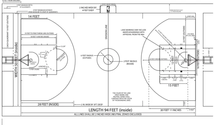
act of doing this is known as “shooting” and in statistics is known as a field goal attempt. The basketball is spherically shaped (29.5-inch circumference in the NBA) and made out of a rubber-like composite material while there are two hoops placed at the center of each short-end of the floor. In the original game, all baskets made during running-clock game play were worth two points, but after the NBA-ABA merger, the NBA adopted rules to award three points for shots (attempts) made from longer distances. A full diagram of the modern NBA court can be found in Figure 1. Upon a successful field goal attempt, the

team that did not score in-bounds the ball from behind the basket they are defending, but after a missed field goal attempt, the ball is considered to be live. The team compete to gain control of the ball, the action of completing this is called a rebound.

Figure 1: NBA Court Dimensions as per the NBA 2018-2019 Rulebook

Players possessing the ball must bounce it while moving and must stay in-bounds. Not doing so would be an example of a violation, punished by loss of possession. Some violations, such as overly physical contact with another player will result in a foul being called on the offending player. In the NBA, accumulating 6 fouls over the course of the

the basic game mechanics and is not exhaustive. The full set of current rules can be found online at the NBA’s website [6].

1.3 Problem Statements

1.3.1

Team Structure and Roster Construction

The first topic of this paper is to address questions in team structure and roster construction. As stated, each team is composed of five active players on the court at a time. What characteristics and attributes of players complete an optimal set of five players is an open question today more than ever before [7].

As basketball became more popular in the 1960’s, the most desired abilities arguably were size and strength to be able to assert oneself in the area close to the basket and score despite physical contact. These traits also would allow one to be equally or more effective on the defensive side of the basket to prevent smaller or weaker opponents from taking close-range shots. Finally, these characteristics would also allow one to be more effective at competing for and winning rebounds. Evidence supporting these notions includes examples of specific players such as Wilt Chamberlain and Bill Russell that epitomized these characteristics and had great individual and team success [8].

“Shooters” with the ability to hit more difficult long-range shots provided value in

that the opposing team would have a larger area of the court to defend as the result, and this ability became even more important with the advent of the three-point line in the 1970’s and 1980’s [3]. Dribbling and passing abilities are the last two major characteristics considered when characterizing players on offense [9].

In name, basketball players had been categorized amongst three positions – guards, forwards, and centers. These classifications were largely determined by height and weight. Guards are typically the shortest and lightest, and centers are typically the tallest and

heaviest [10]. There has also been historical archetypes in roles – guards are typically quickest, best at dribbling the ball, and better at shooting from long distances from the basket. Centers, meanwhile, are typically best at scoring from close range and interior defense due to their advantages in height and weight [11].

The positions of guard and forward are further split up into the following: point guards, shooting guards, small forwards, and power forwards. In terms of player responsibilities, point guards typically specialize in ball handling while shooting guards specialize in shooting. Power forwards specialize in interior defense and rebounding (closer to a center) whereas small forwards typically are quicker and better shooters (closer to a guard). Given the similarity of centers and power forwards, it is common (especially in American collegiate basketball) to play with three designated guards and two forwards, or two guards and three forwards.

These position names and archetypes were created before the invention of the three-point line but remain almost the same today. In the last decade, though, the traditional three and five-type categorizations have come under heavier scrutiny. Especially to those who subscribe to the idea of “positionless basketball,” these categories are almost useless. However, a new framework for understanding types of players has yet to be developed. Another cause for the breakdown of the traditional archetypes is that older stereotypes in player abilities have broken down. Taller and heavier players are able to shoot long-range shots, complete difficult passes with greater awareness, and dribble the ball more than ever before. Meanwhile, the notion that heavier players are better defensive players has never been less true than it is today [7].

In this paper, we will seek to employ machine learning techniques towards identifying player types in the modern NBA. The problem of grouping similar players

1.3.2

Decision Making vs. Skill: Shot Selection &

Shooting Ability

Old-school basketball scouts and analysts would use shooting percentages such as field goal percentage, three-point percentage, and free throw percentage in addition to the vague “eye-test” when assessing a player’s shooting ability. In 2012, Kirk Goldsberry

introduced “CourtVision,” which formally utilized shot location in analyzing shooting ability [12].

Figure 2: Spatial analysis of NBA shots from 2006-2011 by Goldsberry [12]

In 2014, Chang et. al demonstrated that the commonly-known version of the problem of assessing shooting ability was really a combination of two subproblems – shot selection and inherent shooting ability [13]. Shot selection is a metric agnostic to the identity of the player shooting the ball. It is the expected value of a field goal attempt given certain attributes. Meanwhile, inherent shooting ability is a metric determining how much better or worse a player is at a particular type of shot than another player of a particular skill level – usually either average or “replacement-level” (the level of skill of a

player that is not on a team’s top five players, similar to the idea of opportunity cost in economics). In their paper, Chang et. al referred to overall shot quality as Effective Field

Goal Percentage (EFG), to shot selection as Effective Shot Quality (ESQ), and to shooting ability as EFG+ [13].

Figure 3: Chang et. al broke down EFG info ESQ and EFG+ [13]

The enhanced data used to separate these components include details such as (x,y) coordinates of shots and defender distance away from the ball, amongst other features. Chang et. al employed techniques including logistic regression, decision trees, and Gaussian process regression to separate these components. In their paper, Chang et. al specifically mentioned that they believed better algorithms to model this problem would be developed, and in this paper, we will seek to employ more complex models to better learn this feature space. In particular, we will analyze the performance of neural networks using a similar feature set.

Chapter 2

Datasets

This chapter details the datasets utilized for this project. The data for this project will come from two main sources. The first source is data from the popular videogame franchise NBA 2K. The second dataset consists of spatial event data from NBA games during the 2016-2017 season.

2

2.1 Player Attribute Data

The NBA 2K series is the most popular basketball video game in the world, and the creators make a great effort to ensure the realistic representation of the players and the game. These efforts by the game creators have been well-documented historically, and are widely recognized as accurate by the public [14]. The attribute data from the game is composed into three main components.

First, the game contains physical attribute data, such as height, weight, and age, that are ground-truth data points. For the purposes of this project, only height and weight are used.

Second, the dataset contains attributes describing the ability of players to perform several basketball-related actions, such as shooting, passing, dribbling, rebounding, and defense. This segment of the dataset is split into 6 main categories: outside scoring, inside scoring, defending, athleticism, playmaking, and rebounding. Each of these categories further has subcategories, and these are listed in Table 1. Each category and each subcategory includes a rating from 0-99.

Third, the dataset contains player tendency data. This data is split into nine categories and further into subcategories. Unlike the previous attribute dataset, though, ratings from 0-99 are only provided for subcategories, not for categories. Categories and subcategories of player tendency data is listed in Table 2.

Category Sub-categories

Outside Scoring Open Shot Mid Contested Shot Mid Off Dribble Shot Mid Open Shot 3pt

Contested Shot 3pt Off Dribble Shot 3pt Shot IQ

Free Throw

Offensive Consistency

Inside Scoring Shot Close

Standing Layup Driving Layup Standing Dunk Driving Dunk Contact Dunk Draw Foul Post Control Post Hook Post Fadeaway Hands

Defending On-ball Defense IQ

Low Post Defense IQ Pick & Roll Defense IQ Help Defense IQ Lateral Quickness Pass Perception Reaction Time Steal Block Shot Contest Defensive Consistency Athleticism Playmaking Rebounding Overall Total Attributes Speed Acceleration Vertical Strength Stamina Hustle Overall Durability Ball Control Passing Accuracy Passing Vision Passing IQ Speed With Ball Offensive Rebound Defensive Rebound Boxout

N/A N/A

Category Sub-categories

Outside Shooting Shoot

Shot Close Shot Mid Shot Three

Contested Jumper Mid Contested Jumper Three Spin Jumper

Step Through Shot Under Basket Shot Pull Up In Transition

Layups Standing Layup

Driving Layup HopStep Layup EuroStep Layup Floater

Use Glass

Dunking Standing Dunk

Driving Dunk Flashy Dunk Alley Oop Putback Dunk Crash Setup Driving Passing

Cont’d-Next Page

Triple Threat Pumpfake Triple Threat Jabstep Triple Threat Idle Triple Threat Shot Setup with Sizeup Setup with Hesitation Drive

Drive Right vs. Left Driving Crossover Driving Spin Driving Stepback Driving Half Spin Driving Double Crossover

Driving Behind the Back Driving Dribble

Hesitation

Driving In and Out No Driving Dribble

Category Sub-categories

Posting Up

Post Shooting

Defending

Move

Attack Strong on Drive Dish to Open Man Flashy Pass

Alley Oop Pass Post Up

Post Back Down Post Aggressive Back Down

Post Face Up Post Spin Post Drive Post Drop Step Post Hop Step Roll vs. Pop Shoot from Post Post Left Hook Post Right Hook Post Fade Left Post Fade Right Post Shimmy Shot Post Hop Shot Post Stepback Shot Post Up and Center On-Ball Steal Pass Interception Contest Shot Block Shot Take Charge Foul Hard Foul

Table 2: Player Tendencies Cont’d

2.2 Spatial Event Data

The NBA has contracted companies that apply computer vision techniques to convert video feeds into structured features representing events during an NBA game – this structure is similar to that of a regular expression. There are two main types of event data created.

The first type is player location data. This data is provided at a 25hz frequency. Each player is identified on the court according to an (X,Y) coordinate plane representing court location, and the ball is identified in an (X,Y,Z) coordinate system.

The second type of data consists of player activity data including dribbles, passes, rebounds, shots, fouls, and more. Complementary data that relates to team statistics and affects the “box-score” is also provided and typically tied to a location-providing timestamp, though these datasets are separate.

The data analyzed in this paper is from the 2016-2017 season but is not complete. The data is also noisy in terms of both locations and time, but we will find subsets of cleaner data and employ statistical methods to further clean the resulting data.

Chapter 3

Methods

In this chapter, we will present methods used for feature engineering, feature selection, clustering, and prediction. For each section we will:

1) present a high-level overview of the method

2) provide example algorithm pseudocode or equations (where applicable) 3) state the parameters that can be tuned (where applicable) and

4) present methods to determine the quality of the model given specific hyperparameters (where applicable)

3

3.1 Engineered Features

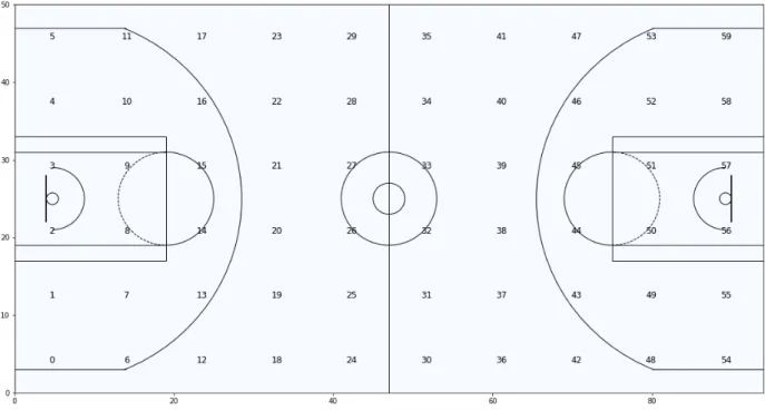
We utilized previous research and input from the Spurs organization to supplement basic practices in engineering specific features from the given set of spatial event data. The first set of engineered features pertained to binning location data into sections of the court. We utilized two grid sizes to split up the court, a ‘tight’ grid and a ‘loose’ grid. The ‘tight’ grid placed a 32x17 grid on the 94-foot x 50-foot court to create roughly 3x3

sections. The advantages of the tight grid are the ability to 1) almost completely separate the corner-three’s from long-two’s 2) isolate the center section of the court directly

perpendicular to the backboards and 3) mirror image on offense and defense. The ‘loose’ version placed a 10x6 grid, which maintained a larger size to help diminish effects of potential noise in the data as well as allow for mirror images of the court in both dimensions. The two grids are shown in Figures 4 and 5.

Finally, research by Chang et al. on shot quality noted distinct features helpful in determining shot quality including shooter velocity and acceleration relative to the vector pointing to the basket. Other features included the distance, velocity, and acceleration of the closest n-defenders with respect to the shooter. In this paper, we set n=3. Our analysis did not include other potentially helpful features such as type of shot or height & weight of shooters and defenders.

Figure 5: Example of ‘loose’ grid-zones

3.2 Principal Component Analysis

We also employed Principal Component Analysis (PCA) to engineer a smaller set of features with higher information content. PCA is a statistical method that converts a set of n observations with p variables that are potentially correlated into a set of linearly uncorrelated variables named principal components (PC’s). By intuition, PCA can be thought of as simply resetting the coordinate plane in the directions of highest variance for a given set of data. The ‘optimal’ coordinate plane outputs ordered orthogonal vectors (in the directions of the eigenvectors of a dataset) in order such that the first vector in the list points in the direction of greatest variance. Each subsequent vector points in the direction of greatest variance and is orthogonal to all previously chosen vectors.

The variance captured by each PC is also explicitly calculated in its eigenvalue. This output gives one the ability to use PCA as a method of feature reduction. Given the set of n observations with p variables centered in matrix X such that each variable pj has

been reshaped to have a mean and standard deviation of 0 and 1 respectively, an algorithm to conduct PCA is shown in Figure 6 where V is an ( n ) x ( n - 1 ) matrix with the eigenvectors as columns and L is an ( n - 1 ) x ( n - 1 ) diagonal matrix of eigenvalues [15].

Figure 6: Steps to compute PCA [15]

The main parameter to tune in PCA is choosing d number of PC’s to select. Feature reduction is typically done such that a particular percentage of the variance is captured by the resulting dimensionality or by choosing the first d components. Feature reduction done in this way also provides an advantage in the ability to reduce noise in the dataset. When possible, we will employ visual representations and examples to show the quality of outputs from PCA and what the outputs represent.

3.3 K-Means Clustering

The K-Means clustering algorithm uses an iterative process to produce a final set of clusters. The algorithm inputs are the number of clusters, k, and the dataset of n observations with p features. The algorithm begins with an initial hypothesis of the

criteria is met. While the algorithm is guaranteed to converge, it may often converge at a local minimum. The pseudocode for k-means is provided in Figure 7 [16].

Figure 7: Lloyd’s Algorithm for K-Means clustering [16]

The input parameters into the model are number of clusters, loss metric, and initialization technique. In this paper, we will use Euclidean Distance as the loss metric and k-means++ as the initialization technique while tuning for the optimal number of clusters.

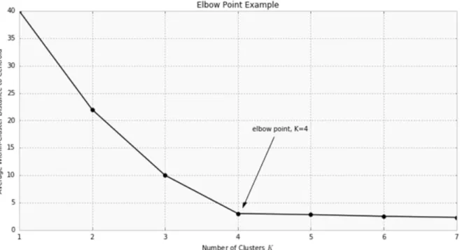
From the generated models, there are several methods to choose an optimal k -value. One such method is the elbow method. Increasing k represents an increase in the parameters of the model and ability to overfit, so one would ideally choose a lower k to preserve the model’s ability to generalize. Meanwhile, increasing k will always decrease the total Euclidean distance (loss) from each data point to the nearest cluster center. The elbow method plots number of clusters, k, on the x-axis versus average within-cluster distance to centroid on the y-axis. One then visually inspects for an ‘elbow point’

representing the optimal number of clusters. An example of using the elbow method is shown in Figure 8.

Figure 8: Example of Applying the Elbow Method

Another method to choose an optimal k is the average silhouette score method. Silhouette analysis gives another metric for cluster separation, and the value ranges between -1 and 1. For this metric, higher values represent that cluster points are highly matched to their own cluster and poorly matched to other clusters. Specifically, the calculation is as follows:

3.4 Gaussian Mixture Models

Gaussian mixture models (GMM’s) are a class of probabilistic models for

representing normally distributed subpopulations within an overall population. GMM’s work well with data that may seem multimodal, meaning that there are several peaks in the data. Figures 9 and 10 demonstrate examples where a GMM would be superior to a single Gaussian distribution.

Figure 9: Sample Potential Use Case of GMM’s in 1D dataset. [19]

Figure 10: Sample Potential Use Case of GMM’s in 2D dataset. [19]

GMM’s also have the added benefit when clustering multidimensional datasets in

offer that is not available in the K-means algorithm, as the K-means algorithm treats each direction equally when determining loss. An example of when this property could be useful is shown in Figure 11.

Figure 11: GMM example where each cluster maintains a unique shape to fit data [20]

Similar to the K-means algorithm, tuning GMM’s involves a two-step process called Expectation Maximization (EM). The individual steps are known as the E-step and the M-step. In the E-step, the algorithm calculates the expectation of component assignments for each data point. In the M-step, the algorithm maximizes expectations calculated in the E-step. Specific instructions for initialization and each step are as follows [18]:

2) E-Step:

3) M-Step:

The main parameter to tune for GMM’s is the value of k, or the number of clusters. The two metrics we used to judge goodness-of-fit are the Akaike Information Criterion (AIC) and Bayesian Information Criterion (BIC). AIC = 2k – 2ln(L) where k is the

number of clusters, or parameters, and L is the maximum value of the model’s likelihood

function. Meanwhile, BIC = ln(n)k – 2ln(L) where n is the sample size. The main difference between the criterion lies in the penalty for number of clusters k. Proponents of BIC suggest that it is best to find the true model, as the probability to do just that approaches 1 as n approaches infinity. Proponents of AIC state that the true model is not often even in the set of candidates, and given finite n, BIC has substantial risk of selecting a poor model [21]. We will use both metrics in the paper.

3.5 Linear Regression & Logistic Regression

Linear regression is a model for linear transformations between a predictor variable X and a response variable Y. When X is a vector rather than a single scalar, this process is referred to as multiple linear regression. Multiple linear regression with k predictor values such that X = [ x1, x2, x3, … xk ] can be written as:

or

In this equation, e represent the residual terms of the model. Linear regression can be thought of finding b such that e2 _{is minimized – this technique is known as Ordinary}

Least Squares [21]. The term we seek to minimize is:

Taking the derivative with respect to b and setting the result equal to 0, we see that:

By doing so, we can include regularization terms to help prevent overfitting. Two popular techniques are either penalizing the sum of the squares of the coefficients or the sum of the absolute values of the coefficients – these techniques are referred to as Ridge Regression and Lasso, respectively.

Logistic regression is similar to linear regression, but seeks to fit a linear function to the log of the odds of outcomes, or the logit function. The logit function ensures estimated outcomes fall in the range (0,1). The base relationship between dependent and independent variables in logistic regression is:

where y is the outcome, xn is the input and wn are the weights. In this setup, w0 represents

the bias term, rather than including it in the weight vector as we saw with b0. As with

linear regression, we can apply regularization to penalize the coefficients or weights.

3.6 Neural Networks & Deep Learning

Neural networks use gradient descent and non-linear transformations to find complex relationships between inputs and outputs. Neural networks can either be used for classification or regression, but in this paper, we will focus on the classification use case. The basic unit for any neural network is a node, an example of which is shown below in Figure 12.

Figure 12: Components of a Node in a Neural Network [22]

Several of these nodes are connected into a network, an example of which is shown below in Figure 13.

Figure 13: Sample connection of nodes within a Neural Network [22]

Neural networks are typically initialized with random weights. The resulting output is then compared to the desired output by a loss function. The result of this loss function is then an input to an optimizer that implements gradient descent to adjust the weights for each node for the next iteration. In this paper, we will specifically use the ‘adam’

of a fully-connected layer with leaky-ReLu as our activation function followed by Batch Normalization [24, 25]. Our output activation function will be the sigmoid function to ensure that all outputs fall within the range (0,1). All other parameters will be tuned. We will use two loss functions, binary cross-entropy and mean squared error, but we will use mean squared error to compare our findings to previous work in the field.

Chapter 4

Results & Discussion

4

In this section, we will first show and discuss results related to the problem of team structure and roster construction. We will then present and discuss results related to shot quality metrics.

4.1 Team Structure and Roster Construction

We will first present results regarding current position classification in the NBA. We will then show the results of using statistical techniques to create relevant player attributes from the spatial event data that can be thought of as player ‘footprints’. We will then apply clustering methods previously mentioned to each dataset to find optimal clusters of players.

small forwards, power forwards, and centers. To this end, we first normalized the dataset using mean and standard deviation of each feature and ran PCA. We then plotted the first three principal components on 2D-axes and color-coded the primary position of each player, shown in Figures 14 and 15.

Figure 14: Position Classification graphed on PC’s 1 and 2 of NBA 2K Dataset

The charts show that the current classification of players can be clearly represented along a linear axis, and in fact, the second and third PC’s offer little to no information regarding the present-day understood positions. PCA showed that the first component represented 29% of the variance in the dataset. While this linear representation of the first principal component categorized to a number of positions equivalent to the number of players on a team allows for a simple user interpretation, one would assume there is a more complex underlying structure interpretable by and useful to a basketball analyst such as a General Manager or Coach. Table 3 shows the largest contributors to the 1st PC and match the original stipulation that positions are largely determined based on attributes correlated with height and weight.

Attribute Corr. with 1st _PC

Ball Control Speed With Ball Off Dribble Shot 3pt Passing Accuracy Drive Crossover Acceleration

Off Dribble Shot Mid Drive Stepback

Drive Dribble Hesitation Contested Shot 3pt Speed Defensive Rebound Putback Dunk Boxout Post Hook Offensive Rebound Low Post Defense IQ Under Basket Shot

-0.9031 -0.899 -0.8561 -0.8327 -0.8116 -0.7983 -0.7712 -0.748 -0.739 -0.7097 -0.697 0.7702 0.7768 0.7964 0.8145 0.825 0.8256 0.8381

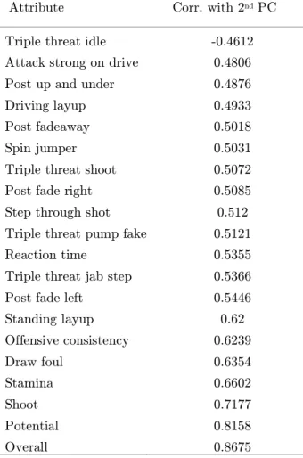
Attribute Corr. with 2nd _PC

Triple threat idle Attack strong on drive Post up and under Driving layup Post fadeaway Spin jumper Triple threat shoot Post fade right Step through shot Triple threat pump fake Reaction time

Triple threat jab step Post fade left

Standing layup Offensive consistency Draw foul Stamina Shoot Potential Overall -0.4612 0.4806 0.4876 0.4933 0.5018 0.5031 0.5072 0.5085 0.512 0.5121 0.5355 0.5366 0.5446 0.62 0.6239 0.6354 0.6602 0.7177 0.8158 0.8675

Attribute Corr. with 3rd _PC

On-ball defensive IQ Help defense IQ Shot contest Pass perception Pick & roll defense IQ Steal

On-ball steal

Defensive consistency Lateral quickness Roll vs. pop

Contested jumper mid Pull up in transition Offensive consistency Shot three Post fadeaway Contested shot 3pt Open shot 3pt Free throw Open shot mid Contested shot mid

-0.4633 -0.4567 -0.4538 -0.4486 -0.4467 -0.4222 -0.4062 -0.3927 -0.3808 -0.3612 0.3356 0.3374 0.3694 0.4116 0.4363 0.4405 0.4478 0.4516 0.4559 0.5107

Table 5: Correlation of NBA 2K Data with 3rd _PC

4.2 Player Attributes from Spatial Data

We organized event data pertaining to player location, shooting, dribbling, passing, and rebounding, and then, we normalized each player’s distribution. Next, we used PCA to find patterns amongst all players and create relevant features for each player. The

4.2.1

Offensive Half-Court Data

We first organized every player’s location while in an offensive half-court setting, defined as a time when all players are on the same half of the floor, the particular player is on the offensive half of the court, and the game-clock is running. We then binned this data per player as per our ‘tight’ gridding system (16 x 17 in a half court setting), effectively creating a location-distribution vector for each player. We then normalized each player’s data such that the value for any bin was the percent of time that a player was recorded in that bin in either an offensive half-court setting. We then conducted PCA on the resulting matrix of all players’ offensive location-distribution vectors and plotted the resulting principal components in Figure 16 and Figure 17.

Figure 17: Player Footprints for Offensive Half-Court Location (PC’s 5-8)

PCA does not return deterministic directionality, so positive and negative results are interchangeable in these plots, and purely represent opposing features. Each PC presented here shows a particular dichotomy of tendencies. The 1st _{PC shows players}

typically either are located outside/near or inside the three-point line. The 2nd _{PC shows}

players typically will either be located at the top of the key by half-court or in the corners. The 3rd _{PC shows a dichotomy between players who are consistently tracking the}

complementary: each show a dichotomy between staying on the right wing vs. the left, and a tendency to run the baseline. The 6th _{PC separates players who hang out in all}

three positions mentioned in the 2nd _{PC vs. those who typically are located at the elbows}

in a half court setting. The 7th _{and 8}th _{PC’s are also somewhat complementary,}

representing players that hang out inside the corner three or beyond the wing-three’s

rather than in the middle or the edges of the court. These eight PC’s are able to represent over 56% of the variation as the full 272-dimensional original vector.

4.2.2

Defensive Half-Court Data

We conducted the same analysis with defensive half-court locations, and produced the following principal component charts in Figure 18. The first two components match almost exactly to the expected defensive-complements of the first two offensive components – the center of each concentrated cluster is between the corresponding cluster in the offensive component and the basket. The 3rd _{component shows a dichotomy between}

players that spend time at the top of the key on defense vs. those who guard wings. The 4th _{component seems to be skewed by two heavily concentrated areas by half-court. Only}

the first three PC’s appear to be relevant – these three PC’s represent just over 31% of the variation as the full 272-dimensional original vector.

Figure 18: Player Footprints for Defensive Half-Court Location (PC’s 1-4)

4.2.3

Shooting Data

Shooting location data was collected similarly to location data, but without the half-court filter. Principal components derived from normalized data for field-goals-attempted and field-goals-made were created. Principal components were also derived from a vector representing each player’s field goal percentage in each location of the court. Unlike previous features, field goal percentages were not normalized relative to the entire

vector prior to PCA, but each feature was still normalized with reference to its distribution amongst all players. All of the original vectors have 272 dimensions representing only the offensive half of the court.

4.2.3.1 Field Goals Made & Field Goals Missed

The 1st _{principal component presents a dichotomy between players who make}

three’s primarily versus those who primarily score very close to the basket. The 2nd

component separates players who shoot midrange jumpers versus those that shoot layups and threes. The 3rd _{component shows a difference between players who take shorter and}

longer threes. This component also shows a light dichotomy between players who make jumpers near the baseline versus those who will shoot from just inside the free throw line. The 4th _{component appears to show a narrow difference between players who make threes}

closer to ‘straight on’ versus those who will make threes from the deeper wings. These components represent just over 11% of the variation of the entire 272-D vector. The first three components of Field Goals Missed appears to correspond well against the first three of field goals made; however, the fourth PC does not show a particularly compelling chart. The first three PC’s represent just over 8% of the variation.

Figure 20: Player Footprints for Field Goals Missed (PC’s 1-4)

4.2.3.2 Field Goal Percentage

4.2.4

Rebounding

Rebounding data was collected similarly to shooting data. Each offensive and defensive rebounding seem to only show one pertinent PC; however, even these each represent less than 4% of the full variation.

4.2.5

Passing and Dribbling

We similarly collected data for each action of throwing passes, receiving passes, and dribbling. For passing attributes, we created full-court plots – vectors with 544 dimensions (32x17 grid size), as we found each of the offensive and defensive components to also be correlated. For dribbling, we found uncorrelated offensive and defensive components, so we chose to plot these separately.

4.2.5.1 Throwing Passes

For passes thrown (inclusive of chest passes and bounce passes), we found three main footprints were legible. The 1st _{component presents a dichotomy between players}

that pass the ball as they are bringing the ball up-court or are on the wing vs. players that rebound in the opposing paint and pass from just above each elbow of the court. The 2nd _{component shows a general split between passing behind half-court and in front of}

half-court. The 3rd _{component shows a split between players that pass in the middle-third}

of the court versus those who pass from the far wings. Each component is plotted in Figure 23.

4.2.5.2 Receiving Passes

For passes received, we found two main footprints were legible. The 1st _component

presents a dichotomy corresponding to the 1st _{component of passes thrown. The 2}nd

component shows a general split between players that receive outlet passes and passes towards the paint vs. those who receive passes on the wings or in the corners. These two footprints are shown in Figure 24.

Figure 23: Player Footprints for Passes Received (PC’s 1-2)

4.2.5.3 Dribbling

For dribbling, we found two main patterns were recognized on each the offensive and defensive halves of the floor. On the defensive end, the 1st _{PC showed a similar}

dichotomy to what we saw on the defensive end in the passing footprints. The 2nd

component appears to represent tendencies to either bring the ball up the center of the court or to bring the ball up-court on either side of the floor. On offense, the 1st _{PC is a}

strong dichotomy between dribbling inside and outside the three-point line. Meanwhile, the 2nd _{PC represents a preference again to dribble along the wing-three regions vs. in the}

center of the court and in the lane.

4.3 Discovering Player Types from NBA 2K Player Data

We utilized clustering techniques on the NBA 2K Player Data in order to discover natural player types. Results from K-Means Clustering and GMM’s are presented in this section.

4.3.1

K-Means Clustering

Because K-means is dependent on scaling of features and number of features in order to create clusters, we first ran PCA on an unscaled dataset. The dataset was input unscaled as each attribute is already provided on a scale of 0-100, and scaling the data to our particular sample would not allow the clustering to fit future samples. We found that the first 18 PC’s accounted for 90% of the variance, and chose to keep those 18 PC’s as features. K-means was run on all cluster sizes from 2 to 30 on this. For each cluster size, up to 30 initializations were tested from k-means++ and the best model was chosen. The plots for the elbow method and silhouette method are shown below in Figure 24 and Figure 25. While the elbow method does not show any obvious result, the silhouette method suggests k=5, k=7, and k=10 are all potential sets of clusters. Detailed silhouette plots for these three values of k are shown in Figures 26-28. For each of these figures, the top left plot is the silhouette plot, the bottom left plot charts each cluster center against height and weight, and the charts on the right plot the clusters with PC’s as each axis. These figures are followed by tables giving defining players for each cluster according to three different metrics.

Table 6: Cluster defining players by three methods for k=5: Minimum scaled Euclidean distance to cluster center (top), maximum sum of distances from player to other cluster centers (middle), maximum difference in distance from player to 2nd _{closest cluster}

Table 7: Cluster defining players by three methods for k=7: Minimum scaled Euclidean distance to cluster center (top), maximum sum of distances from player to other cluster centers (middle), maximum difference in distance from player to 2nd _{closest cluster}

4.3.2 Gaussian Mixture Models

We also utilized Gaussian Mixture Models on the full dataset scaled by the mean and standard deviation of each feature. We were more comfortable using the full dataset as GMM’s are able to have variable sensitivities to each feature for each cluster. For

k=2 to k=25, we initialized 9 GMM’s and plotted the average silhouette score as shown in Figure 29. We also plotted the BIC and AIC for each model, shown in Figure 30.

Figure 29: Average Silhouette Scores for GMM Models

Figure 30: AIC and BIC for GMM Models

The Silhouette plot suggests k=5 could be optimal, but both AIC and BIC suggest larger k. BIC suggests a global minimum at 10 clusters, while AIC shows a

global minimum at 16 clusters. Below is a description of the set of 10 clusters that appeared most often. We chose to detail 10 here as it was the midpoint and BIC is typically more generalizable than AIC. For the BIC Optimal cluster arrangement at n=10, the following clusters were observed (in no particular order):

• Ball-handling backup point guards • Superstar talents

• Rebounding-oriented big men

• Point-guards with a tendency to “score-first”

• Wings that satisfy one of the two criteria in “3 and D” • More athletic big men with a tendency to shoot outside • Backup big-men

• More-skilled “3 and D” wings • Developmental guards and wings

• Guards and wings that have the abilities to shoot, handle the ball, and defend well but are not superstars

What is quite interesting about both results from GMM and K-Means is the distinct classification not only by abilities to shoot, rebound, pass, etc., but also by the overall skill level of the player.

squared error metric for goodness-of-fit. In addition to this metric, we also plotted the resulting model on contrived and real examples to visually see if the model generalized well.

4.4.1 Linear Models

The first test was a training linear model using OLS with just a normalized feature set. The model created had a training error of .2301 and a test error of .2200; however, the visual inspection of the model was less encouraging. Below is a contrived model and three real-game examples. In each chart below, the yellow dots represent the positions of the defenders (in the contrived example labeled ‘open shot test’, all five defenders are in the corner away from the basket). The green dot represents the shooter’s position, the orange dot represents the ball, and the black dots represent the

shooter’s teammates (though, none of these players affect inputs). The black ‘x’ is the point where the ball was shot. These shot charts are created by inputting that the shooter is instead in each other location on the court and recalculating the relevant features, such as closest defender distance, etc. For all examples, the shooter, shot location, and ball location are assumed to be identical (the green dot, black ‘x’ and orange dot all are all assumed to be in the exact same location) and the ball is assumed to be shot at a height of 9.2 feet (the median shot height). In the real-world examples, the shooter maintains their velocity and acceleration measures in every calculation. In the contrived example, all of these metrics are assumed to be 0, as are the corresponding metrics for each defender.

The main problem for the basic linear models appears to be that the significance of the average shooting percentage (or the y-intercept for which these models solve) outweighs a direct relationship between shot-distance and shooting percentage. Ridge Regression and Lasso regularization techniques show little improvement.

Figure 31: Shot Charts for Basic Linear Model (OLS)

There is improvement, however, when we increase the feature set to include 2nd

degree polynomial combinations. A linear ridge-regression model with 10-fold cross-validation is able to visually generalize better and partially overcome the intercept issue.

Figure 32: Shot Charts for Ridge Regression Model with Polynomial Features (n=2)

4.4.2 Neural Networks

We found that we were able to significantly improve on linear models with neural networks while also improving ability to generalize. For our neural network architecture, we calibrated number of hidden layers, batch size, dropout, and layer size. We found that having one hidden layer, low dropout per layer (less than 10%), and a batch size

from 512 to 4096 generally led to better results. The loss metric and layer size seemed to show less significance.

The results from one such model is shown below. This particular model has a training error of .2134, a test error of .2010, and generalizes as shown in the plots below.

Chapter 5

Conclusion

The results in the previous chapter

1) show that the traditional understanding of positions in basketball is largely explained by a single variable

2) present human-understandable player attributes that can be derived from spatial event data without being manually created

3) provide a framework around utilizing unsupervised machine learning techniques towards creating modern player archetypes and

4) demonstrate that deep learning techniques can be utilized to create better models for shot quality.

Bibliography

[1] “Basket Football Game.” Springfield Republican. Springfield, Massachusetts. March 12, 2002.

[2] Goldaper, Sam. “The First Game.” www.nba.com.

[3] “Remember the ABA.” www.remembertheaba.com.

[4] Forbes. “National Basketball Association Total League Revenue* from 2001/02 to

2017/18 (in Billion U.S. Dollars).” Statista - The Statistics Portal, Statista, www.statista.com/statistics/193467/total-league-revenue-of-the-nba-since-2005/ [5] Badenhausen, Kurt. “NBA Team Values 2019: Knicks On Top At $4 Billion.”

Forbes, Forbes Magazine, 21 Feb. 2019,

www.forbes.com/sites/kurtbadenhausen/2019/02/06/nba-team-values-2019-knicks-on-top-at-4-billion/#2a8168cde667.

[6] “2018-19 NBA Rulebook.” 2018-19 NBA Rulebook, National Basketball Assocation, official.nba.com/rulebook/.

[7] Associated Press. “Tweener No More: Versatility Wanted in Positionless NBA.” ESPN, 5 July 2017, www.espn.com/espn/wire/_/section/nba/id/19835157.

[10] “The Average Height of NBA Players - From Point Guards to Centers.” The Hoops Geek, 15 Dec. 2018, www.thehoopsgeek.com/average-nba-height/. [11] “BBC Sport Academy.” BBC News, BBC,

news.bbc.co.uk/sportacademy/bsp/hi/basketball/rules/players/html/default.stm. [12] Goldsberry, Kirk. ”CourtVision: New Visual and Spatial Analytics for the NBA.”

2012 MIT Sloan Sports Analytics Conference. Vol. 9. 2012.

[13] Chang, Yu-Han, et al. ”Quantifying Shot Quality in the NBA.” Proceedings of the 8th Annual MIT Sloan Sports Analytics Conference. MIT, Boston, MA. 2014. [14] Wong, K. (2018, June 01). This Is How NBA 2K Determines Player Rankings.

Retrieved from https://www.complex.com/sports/2017/10/how-nba-2k-determines-player-rankings.

[15] Zafeiriou, Stefanos. “Notes on Implementation of Component Analysis

Techniques.” 2015).

[16] Adams, Ryan P. “K-Means Clustering and Related Algorithms.” Princeton University. 2018.

[17] Trevino, Andrea. “Introduction to K-Means Clustering.” Oracle + DataScience.com, 2016, www.datascience.com/blog/k-means-clustering. [18] “Gaussian Mixture Model.” Brilliant Math & Science Wiki,

brilliant.org/wiki/gaussian-mixture-model/.

[19] “2.1. Gaussian Mixture Models.” Scikit-learn Developers, scikit-learn.org/stable/modules/mixture.html#gmm.

[20] “Akaike Information Criterion.” Wikipedia, Wikimedia Foundation, 1 May 2019,

en.wikipedia.org/wiki/Akaike_information_criterion.

[21] Bremer, M. “Multiple Linear Regression.” Cornell University. 2012.

[22] “A Beginner’s Guide to Neural Networks and Deep Learning.” Skymind, skymind.ai/wiki/neural-network.

[23] Kingma, Diederik P., and Jimmy Ba. ”Adam: A Method for Stochastic Optimization.” arXiv preprint arXiv:1412.6980 (2014).

[24] Xu, Bing, et al. ”Empirical Evaluation of Rectified Activations in Convolutional Network.” arXiv preprint arXiv:1505.00853 (2015).

[25] Ioffe, S. and Szegedy, C. Batch normalization: Accelerating Deep Network Training by Reducing Internal Covariate Shift. Journal of Machine Learning Research, 37:448–456, 2015. http://jmlr.org/proceedings/papers/v37/ioffe15.pdf. Proceedings of the 32nd International Conference on Machine Learning