Publisher’s version / Version de l'éditeur:
Vous avez des questions? Nous pouvons vous aider. Pour communiquer directement avec un auteur, consultez la première page de la revue dans laquelle son article a été publié afin de trouver ses coordonnées. Si vous n’arrivez pas à les repérer, communiquez avec nous à [email protected].
Questions? Contact the NRC Publications Archive team at
[email protected]. If you wish to email the authors directly, please see the first page of the publication for their contact information.
https://publications-cnrc.canada.ca/fra/droits
L’accès à ce site Web et l’utilisation de son contenu sont assujettis aux conditions présentées dans le site LISEZ CES CONDITIONS ATTENTIVEMENT AVANT D’UTILISER CE SITE WEB.
Proceedings of The 12th International Workshop on Semantic Evaluation, pp.
1-17, 2018
READ THESE TERMS AND CONDITIONS CAREFULLY BEFORE USING THIS WEBSITE.
https://nrc-publications.canada.ca/eng/copyright
NRC Publications Archive Record / Notice des Archives des publications du CNRC :
https://nrc-publications.canada.ca/eng/view/object/?id=560b602a-37a5-47be-b306-4b80277382ea https://publications-cnrc.canada.ca/fra/voir/objet/?id=560b602a-37a5-47be-b306-4b80277382ea
NRC Publications Archive
Archives des publications du CNRC
This publication could be one of several versions: author’s original, accepted manuscript or the publisher’s version. / La version de cette publication peut être l’une des suivantes : la version prépublication de l’auteur, la version acceptée du manuscrit ou la version de l’éditeur.
For the publisher’s version, please access the DOI link below./ Pour consulter la version de l’éditeur, utilisez le lien DOI ci-dessous.
https://doi.org/10.18653/v1/S18-1001
Access and use of this website and the material on it are subject to the Terms and Conditions set forth at
SemEval-2018 Task 1: Affect in tweets
Mohammad, Saif; Bravo-Marquez, Felipe; Salameh, Mohammad;
Kiritchenko, Svetlana
Proceedings of the 12th International Workshop on Semantic Evaluation (SemEval-2018), pages 1–17
SemEval-2018 Task 1: Affect in Tweets
Saif M. Mohammad National Research Council Canada
Felipe Bravo-Marquez
The University of Waikato, New Zealand
Mohammad Salameh Carnegie Mellon University in Qatar
Svetlana Kiritchenko National Research Council Canada
Abstract
We present the SemEval-2018 Task 1: Affect in Tweets, which includes an array of subtasks on inferring the affectual state of a person from their tweet. For each task, we created labeled data from English, Arabic, and Spanish tweets. The individual tasks are: 1. emotion intensity regression, 2. emotion intensity ordinal classi-fication, 3. valence (sentiment) regression, 4. valence ordinal classification, and 5. emotion classification. Seventy-five teams (about 200 team members) participated in the shared task. We summarize the methods, resources, and tools used by the participating teams, with a focus on the techniques and resources that are particularly useful. We also analyze systems for consistent bias towards a particular race or gender. The data is made freely available to further improve our understanding of how peo-ple convey emotions through language.
1 Introduction
Emotions are central to language and thought. They are familiar and commonplace, yet they are complex and nuanced. Humans are known to per-ceive hundreds of different emotions. Accord-ing to the basic emotion model (aka the categor-ical model) (Ekman, 1992; Plutchik, 1980; Par-rot, 2001; Frijda, 1988), some emotions, such as joy, sadness, and fear, are more basic than others—physiologically, cognitively, and in terms of the mechanisms to express these emotions. Each of these emotions can be felt or expressed in varying intensities. For example, our ut-terances can convey that we are very angry, slightly sad, absolutely elated, etc. Here, inten-sity refers to the degree or amount of an emo-tion such as anger or sadness.1 As per the
valence–arousal–dominance (VAD) model (Rus-sell, 1980, 2003), emotions are points in a
1Intensity is different from arousal, which refers to the
extent to which an emotion is calming or exciting.
three-dimensional space of valence (positiveness– negativeness), arousal (active–passive), and domi-nance (dominant–submissive). We use the term af-fect to refer to various emotion-related categories such as joy, fear, valence, and arousal.
Natural language applications in commerce, public health, disaster management, and public policy can benefit from knowing the affectual states of people—both the categories and the intensities of the emotions they feel. We thus present the SemEval-2018 Task 1: Affect in Tweets, which includes an array of subtasks where automatic systems have to infer the affectual state of a person from their tweet.2 We will refer to
the author of a tweet as the tweeter. Some of the tasks are on the intensities of four basic emotions common to many proposals of basic emotions: anger, fear, joy, and sadness. Some of the tasks are on valence or sentiment intensity. Finally, we include an emotion classification task over eleven emotions commonly expressed in tweets.3 For
each task, we provide separate training, develop-ment, and test datasets for English, Arabic, and Spanish tweets. The tasks are as follows:
1. Emotion Intensity Regression (EI-reg): Given a tweet and an emotion E, determine the inten-sity of E that best represents the mental state of the tweeter—a real-valued score between 0 (least E) and 1 (most E);
2. Emotion Intensity Ordinal Classification (EI-oc): Given a tweet and an emotion E, classify the tweet into one of four ordinal classes of intensity of E that best represents the mental state of the tweeter;
3. Valence (Sentiment) Regression (V-reg): Given a tweet, determine the intensity of sentiment or valence (V) that best represents the mental state
2https://competitions.codalab.org/competitions/17751 3Determined through pilot annotations.
of the tweeter—a real-valued score between 0 (most negative) and 1 (most positive);
4. Valence Ordinal Classification (V-oc): Given a tweet, classify it into one of seven ordinal classes, corresponding to various levels of positive and negative sentiment intensity, that best represents the mental state of the tweeter; 5. Emotion Classification (E-c): Given a tweet,
classify it as ‘neutral or no emotion’ or as one, or more, of eleven given emotions that best represent the mental state of the tweeter. Here, E refers to emotion, EI refers to emotion intensity, V refers to valence, reg refers to regres-sion, oc refers to ordinal classification, c refers to classification.
For each language, we create a large single tex-tual dataset, subsets of which are annotated for many emotion (or affect) dimensions (from both the basic emotion model and the VAD model). For each emotion dimension, we annotate the data not just for coarse classes (such as anger or no anger) but also for fine-grained real-valued scores indi-cating the intensity of emotion. We use Best– Worst Scaling (BWS), a comparative annotation method, to address the limitations of traditional rating scale methods such as inter- and intra-annotator inconsistency. We show that the fine-grained intensity scores thus obtained are reliable (repeat annotations lead to similar scores). In to-tal, about 700,000 annotations were obtained from about 22,000 English, Arabic, and Spanish tweets. Seventy-five teams (about 200 team members) participated in the shared task, making this the largest SemEval shared task to date. In total, 319 submissions were made to the 15 task–language pairs. Each team was allowed only one official submission for each task–language pair. We sum-marize the methods, resources, and tools used by the participating teams, with a focus on the tech-niques and resources that are particularly useful. We also analyze system predictions for consistent bias towards a particular race or gender using a corpus specifically compiled for that purpose. We find that a majority of systems consistently assign higher scores to sentences involving one race or gender. We also find that the bias may change depending on the specific affective dimension be-ing predicted. All of the tweet data (labeled and unlabeled), annotation questionnaires, evaluation scripts, and the bias evaluation corpus are made freely available on the task website.
2 Building on Past Work
There is a large body of prior work on sen-timent and emotion classification (Mohammad, 2016). There is also growing work on related tasks such as stance detection (Mohammad et al., 2017) and argumentation mining (Wojatzki et al., 2018; Palau and Moens, 2009). However, there is little work on detecting the intensity of affect in text. Mohammad and Bravo-Marquez (2017) cre-ated the first datasets of tweets annotcre-ated for anger, fear, joy, and sadness intensities. Given a focus emotion, each tweet was annotated for intensity of the emotion felt by the speaker using a technique called Best–Worst Scaling (BWS) (Louviere, 1991; Kiritchenko and Mohammad, 2016, 2017).
BWS is an annotation scheme that addresses the limitations of traditional rating scale methods, such as inter- and intra-annotator inconsistency, by employing comparative annotations. Note that at its simplest, comparative annotations involve giv-ing people pairs of items and askgiv-ing which item is greater in terms of the property of interest. How-ever, such a method requires annotations for N2
items, which can be prohibitively large.
In BWS, annotators are given n items (an n-tuple, where n > 1 and commonly n = 4). They are asked which item is the best (highest in terms of the property of interest) and which is the worst (lowest in terms of the property of interest). When working on 4-tuples, best–worst annotations are particularly efficient because each best and worst annotation will reveal the order of five of the six item pairs. For example, for a 4-tuple with items A, B, C, and D, if A is the best, and D is the worst, then A > B, A > C, A > D, B > D, and C > D. Real-valued scores of association between the items and the property of interest can be de-termined using simple arithmetic on the number of times an item was chosen best and number of times it was chosen worst (as described in Section 3.4.2) (Orme, 2009; Flynn and Marley, 2014).
It has been empirically shown that annotations for 2N 4-tuples is sufficient for obtaining reliable scores (where N is the number of items) (Louviere, 1991; Kiritchenko and Mohammad, 2016). Kir-itchenko and Mohammad (2017) showed through empirical experiments that BWS produces more reliable and more discriminating scores than those obtained using rating scales. (See (Kiritchenko and Mohammad, 2016, 2017) for further details on BWS.)
Mohammad and Bravo-Marquez (2017) col-lected and annotated 7,100 English tweets posted in 2016. We will refer to the tweets alone as Tweets-2016, and the tweets and annotations together as the Emotion Intensity Dataset (or, EmoInt Dataset). This dataset was used in the 2017 WASSA Shared Task on Emotion Intensity.4
We build on that earlier work by first compiling a new set of English, Arabic, and Spanish tweets posted in 2017 and annotating the new tweets for emotion intensity in a similar manner. We will re-fer to this new set of tweets as Tweets-2017. Simi-lar to the work by Mohammad and Bravo-Marquez (2017), we create four subsets annotated for inten-sity of fear, joy, sadness, and anger, respectively. However, unlike the earlier work, here a common dataset of tweets is annotated for all three negative emotions: fear, anger, and sadness. This allows one to study the relationship between the three ba-sic negative emotions.
We also annotate tweets sampled from each of the four basic emotion subsets (of both Tweets-2016 and Tweets-2017) for degree of valence. An-notations for arousal, dominance, and other basic emotions such as surprise and anticipation are left for future work.
In addition to knowing a fine-grained score indicating degree of intensity, it is also useful to qualitatively ground the information on whether the intensity is high, medium, low, etc. Thus, we manually identify ranges in intensity scores that correspond to these coarse classes. For each of the four emotions E, the 0 to 1 range is partitioned into the classes: no E can be inferred, low E can be inferred, moderate E can be inferred, and high E can be inferred. This data can be used for developing systems that predict the ordinal class of emotion intensity (EI ordinal classification, or EI-oc, systems). We partition the 0 to 1 interval of valence into: very negative, moderately negative, slightly negative, neutral or mixed, slightly positive, moderately positive, and very positive mental state of the tweeter can be inferred. This data can be used to develop systems that predict the ordinal class of valence (valence ordinal classification, or V-oc, systems).5 4http://saifmohammad.com/WebPages/EmoInt2017.html 5Note that valence ordinal classification is the traditional
sentiment analysis task most commonly explored in NLP lit-erature. The classes may vary from just three (positive, nega-tive, and neutral) to five, seven, or nine finer classes.
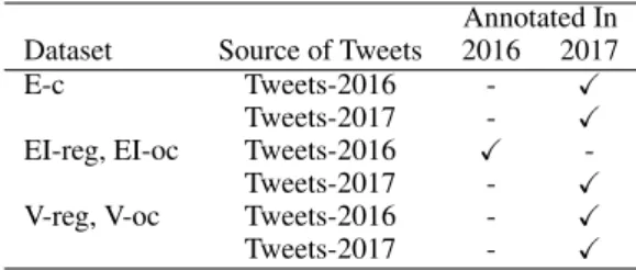
Annotated In Dataset Source of Tweets 2016 2017
E-c Tweets-2016 - X
Tweets-2017 - X
EI-reg, EI-oc Tweets-2016 X
-Tweets-2017 - X
V-reg, V-oc Tweets-2016 - X
Tweets-2017 - X
Table 1: The annotations of English Tweets.
Finally, the full Tweets-2016 and Tweets-2017 datasets are annotated for the presence of eleven emotions: anger, anticipation, disgust, fear, joy, love, optimism, pessimism, sadness, surprise, and trust. This data can be used for developing multi-label emotion classification, or E-c, systems. Ta-ble 1 shows the two stages in which the anno-tations for English tweets were done. The Ara-bic and Spanish tweets were all only from 2017. Together, we will refer to the joint set of tweets from Tweets-2016 and Tweets-2017 along with all the emotion-related annotations described above as the SemEval-2018 Affect in Tweets Dataset (or AIT Dataset for short).
3 The Affect in Tweets Dataset
We now present how we created the Affect in Tweets Dataset. We present only the key details here; a detailed description of the English datasets and the analysis of various affect dimensions is available in Mohammad and Kiritchenko (2018). 3.1 Compiling English Tweets
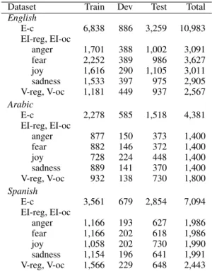
We first compiled tweets to be included in the four EI-reg datasets corresponding to anger, fear, joy, and sadness. The EI-oc datasets include the same tweets as in EI-reg, that is, the Anger EI-oc dataset has the same tweets as in the Anger EI-reg dataset, the Fear EI-oc dataset has the same tweets as in the Fear EI-reg dataset, and so on. However, the labels for EI-oc tweets are ordinal classes instead of real-valued intensity scores. The V-reg dataset includes a subset of tweets from each of the four EI-reg emotion datasets. The V-oc dataset has the same tweets as in the V-reg dataset. The E-c dataset in-cludes all the tweets from the four EI-reg datasets. The total number of instances in the E-c, EI-reg, EI-oc, V-reg, and V-oc datasets is shown in the last column of Table 3.
3.1.1 Basic Emotion Tweets
To create a dataset of tweets rich in a particu-lar emotion, we used the following methodology.
For each emotion X, we selected 50 to 100 terms that were associated with that emotion at differ-ent intensity levels. For example, for the anger dataset, we used the terms: angry, mad, frustrated, annoyed, peeved, irritated, miffed, fury, antago-nism, and so on. We will refer to these terms as the query terms. The query terms we selected in-cluded emotion words listed in the Roget’s The-saurus, nearest neighbors of these emotion words in a word-embeddings space, as well as commonly used emoji and emoticons. The full list of the query terms is available on the task website.
We polled the Twitter API, over the span of two months (June and July, 2017), for tweets that in-cluded the query terms. We randomly selected 1,400 tweets from the joy set for annotation of in-tensity of joy. For the three negative emotions, we first randomly selected 200 tweets each from their corresponding tweet collections. These 600 tweets were annotated for all three negative emo-tions so that we could study the relaemo-tionships be-tween fear and anger, bebe-tween anger and sadness, and between sadness and fear. For each of the negative emotions, we also chose 800 additional tweets, from their corresponding tweet sets, that were annotated only for the corresponding emo-tion. Thus, the number of tweets annotated for each of the negative emotions was also 1,400 (the 600 included in all three negative emotions + 800 unique to the focus emotion). For each emotion, 100 tweets that had an emotion-word hashtag, emoticon, or emoji query term at the end (trailing query term) were randomly chosen. We removed the trailing query terms from these tweets. As a result, the dataset also included some tweets with no clear emotion-indicative terms.
Thus, the EI-reg dataset included 1,400 new tweets for each of the four emotions. These were annotated for intensity of emotion. Note that the EmoInt dataset already included 1,500 to 2,300 tweets per emotion annotated for intensity. Those tweets were not re-annotated. The EmoInt EI-reg tweets as well as the new EI-reg tweets were both annotated for ordinal classes of emotion (EI-oc) as described in Section 3.4.3
The new EI-reg tweets formed the EI-reg de-velopment (dev) and test sets in the AIT task; the number of instances in each is shown in the third and fourth columns of Table 3. The EmoInt tweets formed the training set.6
6Manual examination of the new EI-reg tweets later
re-3.1.2 Valence Tweets
The valence dataset included tweets from the new EI-reg set and the EmoInt set. The new EI-reg tweets included were all 600 tweets common to the three negative emotion tweet sets and 600 ran-domly chosen joy tweets. The EmoInt tweets in-cluded were 600 randomly chosen joy tweets and 200 each, randomly chosen tweets, for anger, fear, and sadness. To study valence in sarcastic tweets, we also included 200 tweets that had hashtags #sarcastic, #sarcasm, #irony, or #ironic (tweets that are likely to be sarcastic). Thus the V-reg set included 2,600 tweets in total. The V-oc set is comprised of the same tweets as in the V-reg set. 3.1.3 Multi-Label Emotion Tweets
We selected all of the 2016 and 2017 tweets in the four EI-reg datasets to form the E-c dataset, which is annotated for presence/absence of 11 emotions. 3.2 Compiling Arabic Tweets
We compiled the Arabic tweets in a similar manner to the English dataset. We obtained the the Arabic query terms as follows:
• We translated the English query terms for the four emotions to Arabic using Google Translate. • All words associated with the four emotions in the NRC Emotion Lexicon were translated into Arabic. (We discarded incorrect translations.) • We trained word embeddings on a tweet corpus
collected using dialectal function words as queries. We used nearest neighbors of the emotion query terms in the word-embedding space as additional query terms.
• We included the same emoji used in English for anger, fear, joy and sadness. However, most of the fear emoji were not included, as they were rarely associated with fear in Arabic tweets. In total, we used 550 Arabic query terms and emoji to poll the Twitter API to collect around 17 million tweets between March and July 2017. For each of the four emotions, we randomly se-lected 1,400 tweets to form the EI-reg datasets. The same tweets were used for building the EI-oc datasets. The sets of tweets for the negative emotions included 800 tweets unique to the focus emotion and 600 tweets common to the three neg-ative emotions.
vealed that it included some near-duplicate tweets. We kept only one copy of such pairs. Thus the dev. and test set num-bers add up to a little lower than 1,400.
The V-reg dataset was formed by including about 900 tweets from the three negative emotions (including the 600 tweets common to the three negative emotion datasets), and about 900 tweets for joy. The same tweets were used to form the V-oc dataset. The multi-label emotion classification dataset was created by taking all the tweets in the EI-reg datasets.
3.3 Compiling Spanish Tweets
The Spanish query terms were obtained as fol-lows:
• The English query terms were translated into Spanish using Google Translate. The transla-tions were manually examined by a Spanish native speaker, and incorrect translations were discarded.
• The resulting set was expanded using synonyms taken from a Spanish lexicographic resource, Wordreference7.
• We made sure that both masculine and fem-inine forms of the nouns and adjectives were included.
• We included the same emoji used in English for anger, sadness, and joy. The emoji for fear where not included, as tweets contain-ing those emoji were rarely associated with fear. We collected about 1.2 million tweets between July and September 2017. We annotated close to 2,000 tweets for each emotion. The sets of tweets for the negative emotions included ∼1,500 tweets unique to the focus emotion and ∼500 tweets common to the two remaining negative emotions. The same tweets were used for building the Span-ish EI-oc dataset.
The V-reg dataset was formed by including about 1,100 tweets from the three negative emo-tions (including the 750 tweets common to the three negative emotion datasets), about 1,100 tweets for joy, and 268 tweets with sarcastic hash-tags (#sarcasmo, #ironia). The same tweets were used to build the V-oc dataset. The multi-label emotion classification dataset was created by tak-ing all the tweets in the EI-reg and V-reg datasets. 3.4 Annotating Tweets
We describe below how we annotated the English tweets. The same procedure was used for Arabic and Spanish annotations.
7http://www.wordreference.com/sinonimos/
We annotated all of our data by crowdsourcing. The tweets and annotation questionnaires were uploaded on the crowdsourcing platform, Figure Eight (earlier called CrowdFlower).8 All the
anno-tation tasks described in this paper were approved by the National Research Council Canada’s Insti-tutional Review Board.
About 5% of the tweets in each task were an-notated internally beforehand (by the authors of this paper). These tweets are referred to as gold tweets. The gold tweets were interspersed with other tweets. If a crowd-worker got a gold tweet question wrong, they were immediately notified of the error. If the worker’s accuracy on the gold tweet questions fell below 70%, they were re-fused further annotation, and all of their annota-tions were discarded. This served as a mechanism to avoid malicious annotations.
3.4.1 Multi-Label Emotion Annotation We presented one tweet at a time to the annotators and asked which of the following options best de-scribed the emotional state of the tweeter:
– anger (also includes annoyance, rage) – anticipation (also includes interest, vigilance) – disgust (also includes disinterest, dislike, loathing) – fear (also includes apprehension, anxiety, terror) – joy (also includes serenity, ecstasy)
– love (also includes affection)
– optimism (also includes hopefulness, confidence) – pessimism (also includes cynicism, no confidence) – sadness (also includes pensiveness, grief) – surprise (also includes distraction, amazement) – trust (also includes acceptance, liking, admiration) – neutral or no emotion
Example tweets were provided in advance with ex-amples of suitable responses.
On the Figure Eight task settings, we specified that we needed annotations from seven people for each tweet. However, because of the way the gold tweets were set up, they were annotated by more than seven people. The median number of tations was still seven. In total, 303 people anno-tated between 10 and 4,670 tweets each. A total of 174,356 responses were obtained.
Annotation Aggregation: One of the criticisms for several natural language annotation projects has been that they keep only the instances with high agreement, and discard instances that obtain low agreements. The high agreement instances
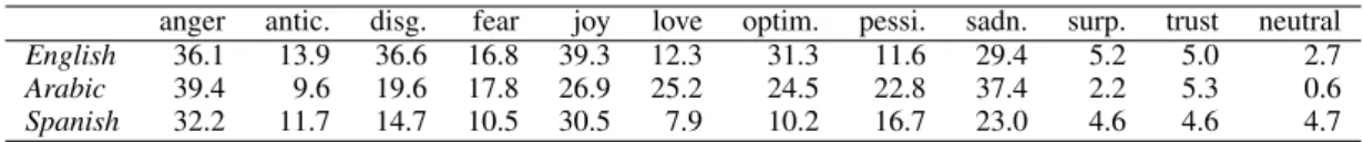
anger antic. disg. fear joy love optim. pessi. sadn. surp. trust neutral
English 36.1 13.9 36.6 16.8 39.3 12.3 31.3 11.6 29.4 5.2 5.0 2.7
Arabic 39.4 9.6 19.6 17.8 26.9 25.2 24.5 22.8 37.4 2.2 5.3 0.6
Spanish 32.2 11.7 14.7 10.5 30.5 7.9 10.2 16.7 23.0 4.6 4.6 4.7
Table 2: Percentage of tweets that were labeled with a given emotion (after aggregation of votes).
tend to be simple instantiations of the classes of interest, and are easier to model by automatic sys-tems. However, when deployed in the real world, natural language systems have to recognize and process more complex and subtle instantiations of a natural language phenomenon. Thus, discarding all but the high agreement instances does not fa-cilitate the development of systems that are able to handle the difficult instances appropriately.
Therefore, we chose a somewhat generous ag-gregation criterion: if more than 25% of the re-sponses (two out of seven people) indicated that a certain emotion applies, then that label was cho-sen. We will refer to this aggregation as Ag2. If no emotion got at least 40% of the responses (three out of seven people) and more than 50% of the re-sponses indicated that the tweet was neutral, then the tweet was marked as neutral. In the vast ma-jority of the cases, a tweet was labeled either as neutral or with one or more of the eleven emotion labels. 107 English tweets, 14 Arabic tweets, and 88 Spanish tweets did not receive sufficient votes to be labeled a particular emotion or to be labeled neutral. These very-low-agreement tweets were set aside. We will refer to the remaining dataset as E-c (Ag2), or simply E-c, data.
Class Distribution: Table 2 shows the percent-age of tweets that were labeled with a given emo-tion using Ag2 aggregaemo-tion. The numbers in these rows sum up to more than 100% because a tweet may be labeled with more than one emotion. Ob-serve that joy, anger, disgust, sadness, and opti-mism get a high number of the votes. Trust and surprise are two of the lowest voted emotions. 3.4.2 Annotating Intensity with BWS
We followed the procedure described by Kir-itchenko and Mohammad (2016) to obtain best– worst scaling (BWS) annotations.
Every 4-tuple was annotated by four indepen-dent annotators. The questionnaires were devel-oped through internal discussions and pilot anno-tations. They are available on the SemEval-2018 AIT Task webpage.
Between 118 and 220 people residing in the United States annotated the 4-tuples for each of
the four emotions and valence. In total, around 27K responses for each of the four emotions and around 50K responses for valence were obtained.9
Annotation Aggregation: The intensity scores were calculated from the BWS responses using a simple counting procedure (Orme, 2009; Flynn and Marley, 2014): For each item, the score is the proportion of times the item was chosen as having the most intensity minus the percentage of times the item was chosen as having the least intensity.10
We linearly transformed the scores to lie in the 0 (lowest intensity) to 1 (highest intensity) range. Distribution of Scores: Figure 1 shows the his-togram of the V-reg tweets. The tweets are grouped into bins of scores 0–0.05, 0.05–0.1, and so on until 0.95–1. The colors for the bins corre-spond to their ordinal classes as determined from the manual annotation described in the next sub-section. The histograms for the four emotions are shown in Figure 5 in the Appendix.
3.4.3 Identifying Ordinal Classes
For each of the EI-reg emotions, the authors of this paper independently examined the ordered list of tweets to identify suitable boundaries that par-titioned the 0–1 range into four ordinal classes: no emotion, low emotion, moderate emotion, and high emotion. Similarly the V-reg tweets were examined and the 0–1 range was partitioned into seven classes: very negative, moderately negative, slightly negative, neutral or mixed, slightly posi-tive, moderately posiposi-tive, and very positive mental state can be inferred.11
Annotation Aggregation: The authors discussed their individual annotations to obtain consensus on the class intervals. The V-oc and EI-oc datasets were thus labeled.
Class Distribution: The legend of Figure 1 shows the intervals of V-reg scores that make up the seven V-oc classes. The intervals of EI-reg scores that make up each of the four EI-oc classes are shown in Figure 5 in the Appendix.
9Gold tweets were annotated more than four times. 10Code for generating tuples from items as well
as for generating scores from BWS annotations: http://saifmohammad.com/WebPages/BestWorst.html
Figure 1:Valence score (V-reg), class (V-oc) distribution. 3.4.4 Annotating Arabic and Spanish Tweets The annotations for Arabic and Spanish tweets fol-lowed the same process as the one described for English above. We manually translated the En-glish questionnaire into Arabic and Spanish.
On Figure Eight, we used similar settings as for English. For Arabic, we set the country of annota-tors to fourteen Arab countries available in Crowd-flower as well as the United States of America.12
For Spanish, we set the country of annotators to USA, Mexico, and Spain.
Annotation aggregation was done the same way for Arabic and Spanish, as for English. Table 2 shows the distributions for different emotions in the E-c annotations for Arabic and Spanish (in ad-dition to English).
3.5 Training, Development, and Test Sets Table 14 in Appendix summarizes key details of the current set of annotations done for the SemEval-2018 Affect in Tweets (AIT) Dataset. AIT was partitioned into training, development, and test sets for machine learning experiments as described in Table 3. All of the English tweets that came from Tweets-2016 were part of the train-ing sets. All of the English tweets that came from Tweets-2017 were split into development and test sets.13The Arabic and Spanish tweets are all from
2017 and were split into train, dev, and test sets.
12 Algeria, Bahrain, Egypt, Jordan, Kuwait, Morocco,
Oman, Palestine, Qatar, Saudi Arabia, Tunisia, UAE, Yemen.
13This split of Tweets-2017 was first done such that 20% of
the tweets formed the dev. set and 80% formed the test set— independently for EI-reg, EI-oc, V-reg, V-oc, and E-c. Then we moved some tweets from the test sets to the dev. sets such that a tweet in any dev. set does not occur in any test set.
Dataset Train Dev Test Total
English E-c 6,838 886 3,259 10,983 EI-reg, EI-oc anger 1,701 388 1,002 3,091 fear 2,252 389 986 3,627 joy 1,616 290 1,105 3,011 sadness 1,533 397 975 2,905 V-reg, V-oc 1,181 449 937 2,567 Arabic E-c 2,278 585 1,518 4,381 EI-reg, EI-oc anger 877 150 373 1,400 fear 882 146 372 1,400 joy 728 224 448 1,400 sadness 889 141 370 1,400 V-reg, V-oc 932 138 730 1,800 Spanish E-c 3,561 679 2,854 7,094 EI-reg, EI-oc anger 1,166 193 627 1,986 fear 1,166 202 618 1,986 joy 1,058 202 730 1,990 sadness 1,154 196 641 1,991 V-reg, V-oc 1,566 229 648 2,443
Table 3: The number of tweets in the SemEval-2018 Affect in Tweets Dataset.
4 Agreement and Reliability of Annotations
It is challenging to obtain consistent annotations for affect due to a number of reasons, including: the subtle ways in which people can express affect, fuzzy boundaries of affect categories, and differ-ences in human experience that impact how they perceive emotion in text. In the subsections below we analyze the AIT dataset to determine the extent of agreement and the reliability of the annotations. 4.1 E-c Annotations
Table 4 shows the inter-rater agreement and Fleiss’ κ for the multi-label emotion annotations. The inter-rater agreement (IRA) is calculated as the percentage of times each pair of annotators agree. For the sake of comparison, we also show the scores obtained by randomly choosing whether a particular emotion applies or not. Observe that the scores obtained through the actual annotations are markedly higher than the scores obtained by ran-dom guessing.
4.2 EI-reg and V-reg Annotations
For real-valued score annotations, a commonly used measure of quality is reproducibility of the end result—if repeated independent manual anno-tations from multiple respondents result in similar
IRA Fleiss’ κ
Random 41.67 0.00
English avg. for all 12 classes 83.38 0.21 avg. for 4 basic emotions 81.22 0.40 Arabic avg. for all 12 classes 86.69 0.29 avg. for 4 basic emotions 83.38 0.48 Spanish avg. for all 12 classes 88.60 0.28 avg. for 4 basic emotions 85.91 0.45
Table 4: Annotator agreement for the Multi-label Emotion Classification (E-c) Datasets.
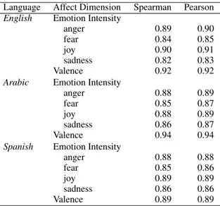
Language Affect Dimension Spearman Pearson English Emotion Intensity
anger 0.89 0.90
fear 0.84 0.85
joy 0.90 0.91
sadness 0.82 0.83
Valence 0.92 0.92
Arabic Emotion Intensity
anger 0.88 0.89
fear 0.85 0.87
joy 0.88 0.89
sadness 0.86 0.87
Valence 0.94 0.94
Spanish Emotion Intensity
anger 0.88 0.88
fear 0.85 0.86
joy 0.89 0.89
sadness 0.86 0.86
Valence 0.89 0.89
Table 5: Split-half reliabilities in the AIT Dataset.
intensity rankings (and scores), then one can be confident that the scores capture the true emotion intensities. To assess this reproducibility, we cal-culate average split-half reliability (SHR), a com-monly used approach to determine consistency (Kuder and Richardson, 1937; Cronbach, 1946; Mohammad and Bravo-Marquez, 2017). The in-tuition behind SHR is as follows. All annotations for an item (in our case, tuples) are randomly split into two halves. Two sets of scores are produced independently from the two halves. Then the cor-relation between the two sets of scores is calcu-lated. The process is repeated 100 times, and the correlations are averaged. If the annotations are of good quality, then the average correlation between the two halves will be high.
Table 5 shows the split-half reliabilities for the AIT data. Observe that correlations lie between 0.82 and 0.92, indicating a high degree of repro-ducibility.14
14Past work has found the SHR for sentiment intensity
an-notations for words, with 6 to 8 anan-notations per tuple to be 0.95 to 0.98 (Mohammad, 2018b; Kiritchenko and Moham-mad, 2016). In contrast, here SHR is calculated from whole sentences, which is a more complex annotation task and thus the SHR is expected to be lower than 0.95.
5 Evaluation for Automatic Predictions
5.1 For EI-reg, EI-oc, V-reg, and V-oc
The official competition metric for EI-reg, EI-oc, V-reg, and V-oc was the Pearson Correlation Coefficient with the Gold ratings/labels. For EI-reg and EI-oc, the correlation scores across all four emotions were averaged (macro-average) to determine the bottom-line competition met-ric. Apart from the official competition metric described above, some additional metrics were also calculated for each submission. These were intended to provide a different perspective on the results. The secondary metric used for the regression tasks was:
• Pearson correlation for a subset of the test set that includes only those tweets with intensity score greater or equal to 0.5.
The secondary metrics used for the ordinal classi-fication tasks were:
• Pearson correlation for a subset of the test set that includes only those tweets with intensity classes low X, moderate X, or high X (where X is an emotion). We will refer to this set of tweets as the some-emotion subset.
• Weighted quadratic kappa on the full test set. • Weighted quadratic kappa on the some-emotion
subset of the test set. 5.2 For E-c
The official competition metric used for E-c was multi-label accuracy (or Jaccard index). Since this is a multi-label classification task, each tweet can have one or more gold emotion labels, and one or more predicted emotion labels. Multi-label accuracy is defined as the size of the intersection of the predicted and gold label sets divided by the size of their union. This measure is calculated for each tweet t, and then is averaged over all tweets T in the dataset: Accuracy = 1 |T | X t∈T Gt∩ Pt Gt∪ Pt
where Gtis the set of the gold labels for tweet t, Pt
is the set of the predicted labels for tweet t, and T is the set of tweets. Apart from the official compe-tition metric (multi-label accuracy), we also calcu-lated micro-averaged F-score and macro-averaged F-score.15
Task English Arabic Spanish All EI-reg 48 13 15 76 EI-oc 37 12 14 63 V-reg 37 13 13 63 V-oc 35 13 12 60 E-c 33 12 12 57 Total 190 63 66 319
Table 6: Number of teams in each task–language pair.
6 Systems
Seventy-five teams (about 200 team members) participated in the shared task, submitting to one or more of the five subtasks. The numbers of teams submitting predictions for each task– language pair are shown in Table 6. The English tasks were the most popular (33 to 48 teams for each task); however, the Arabic and Spanish tasks also got a fair amount of participation (about 13 teams for each task). Emotion intensity regression attracted the most teams.
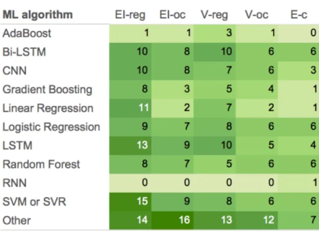
Figure 2 shows how frequently various ma-chine learning algorithms were used in the five tasks. Observe that SVM/SVR, LSTMs and Bi-LSTMs were some of the most widely used al-gorithms. Understandably, regression algorithms such as Linear Regression were more common in the regression tasks than in the classification tasks. Figure 3 shows how frequently various features were used. Observe that word embeddings, af-fect lexicon features, and word n-grams were some of the most widely used features. Many teams also used sentence embeddings and affect-specific word embeddings. A number of teams also made use of distant supervision corpora (usually tweets with emoticons or hashtagged emotion words). Several teams made use of the AIT2018 Dis-tant Supervision Corpus—a corpus of about 100M tweets containing emotion query words—that we provided. A small number of teams used training data from one task to supplement the training data for another task. (See row‘AIT-2018 train-dev (other task)’.)
Figure 4 shows how frequently features from various affect lexicons were used. Observe that several of the NRC emotion and sentiment lexi-cons as well as AFINN and Bing Liu Lexicon were widely used (Mohammad and Turney, 2013; Mo-hammad, 2018b; Kiritchenko et al., 2014; Nielsen, 2011; Hu and Liu, 2004). Several teams used the AffectiveTweets package to obtain lexicon fea-tures (Mohammad and Bravo-Marquez, 2017).16
16https://affectivetweets.cms.waikato.ac.nz/
Figure 2:Machine learning algorithms used by teams.
Figure 3:Features and resources used by teams. 6.1 Results and Discussion
Tables 7 through 11 show the results obtained by the top three teams on EI-reg, EI-oc, V-reg, V-oc, and E-c, respectively. The tables also show: (a) the results obtained by the median rank team for each task–language pair, (b) the results obtained by a baseline SVM system using just word unigrams as features, and (c) the results obtained by a system that randomly guesses the prediction—the random baseline.17 Observe that the top teams obtained
markedly higher results than the SVM unigrams baselines.
Most of the top-performing teams relied on both deep neural network representations of tweets (sentence embeddings) as well as features derived from existing sentiment and emotion lexicons. Since many of the teams used similar models when participating in different tasks, we present further details of the systems grouped by the language for which they submitted predictions.
17The results for each of the 75 participating teams are
shown on the task website and also in the supplementary ma-terial file. (Not shown here due to space constraints.)
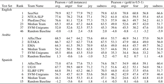
Pearson r (all instances) Pearson r (gold in 0.5-1)
Test Set Rank Team Name avg. anger fear joy sadness avg. anger fear joy sadness English 1 SeerNet 79.9 82.7 77.9 79.2 79.8 63.8 70.8 60.8 56.8 66.6 2 NTUA-SLP 77.6 78.2 75.8 77.1 79.2 61.0 63.6 59.5 55.4 65.4 3 PlusEmo2Vec 76.6 81.1 72.8 77.3 75.3 57.9 66.3 49.7 54.2 61.3 23 Median Team 65.3 65.4 67.2 64.8 63.5 49.0 52.6 49.7 42.0 51.7 37 SVM-Unigrams 52.0 52.6 52.5 57.5 45.3 39.6 45.5 30.2 47.6 35.0 46 Random Baseline -0.8 -1.8 2.4 -5.8 2.0 -4.8 -8.8 -1.1 -3.2 -5.9 Arabic 1 AffecThor 68.5 64.7 64.2 75.6 69.4 53.7 46.9 54.1 57.0 56.9 2 EiTAKA 66.7 62.7 62.7 73.8 67.5 53.3 47.9 60.4 49.0 56.0 3 EMA 64.3 61.5 59.3 70.9 65.6 49.0 44.4 45.7 49.7 56.2 6 Median Team 54.2 50.1 50.1 62.8 53.7 44.6 39.1 43.0 45.4 51.0 7 SVM-Unigrams 45.5 40.6 43.5 53.0 45.0 35.3 34.4 36.6 33.2 36.7 13 Random Baseline 1.3 -0.6 1.6 -1.0 5.2 -0.7 0.2 0.7 1.1 -4.8 Spanish 1 AffecThor 73.8 67.6 77.6 75.3 74.6 58.7 54.9 60.4 59.1 60.4 2 UG18 67.7 59.5 68.9 71.2 71.2 51.6 42.2 52.1 54.0 58.1 3 ELiRF-UPV 64.8 59.1 63.2 66.3 70.5 44.0 41.0 37.5 45.6 51.7 6 SVM-Unigrams 54.3 45.7 61.9 53.6 56.0 46.2 42.9 47.4 47.9 46.4 8 Median Team 44.1 34.8 53.3 41.4 47.1 38.2 24.6 42.5 44.8 41.0 15 Random Baseline -1.2 -5.6 0.4 1.8 -1.4 -0.5 0.1 -4.6 1.8 0.8
Table 7: Task 1 emotion intensity regression (EI-reg): Results.
Figure 4:Lexicons used by teams.
High-Ranking English Systems: The best per-forming system for regression (EI-reg, V-reg) and ordinal classification (EI-oc,V-oc) sub-tasks in English was SeerNet. The team proposed a unified architecture for regression and ordinal classifica-tion based on the fusion of heterogeneous features and the ensemble of multiple predictive models. The following models or resources were used for feature extraction:
• DeepMoji (Felbo et al., 2017): a neural network for predicting emoji for tweets trained from a very large distant supervision corpus. The last two layers of the network were used as features. • Skip thoughts: an unsupervised neural network
for encoding sentences (Kiros et al., 2015). • Sentiment neurons (Radford et al., 2017): a
byte-level recurrent language model for learn-ing sentence representations.
• Features derived from affective lexicons. These feature vectors were used for training XG Boost and Random Forest models (using both re-gression and classification variants), which were later stacked using ordinal logistic regression and ridge regression models for the corresponding or-dinal classification and regression tasks.
Other teams also relied on both deep neural net-work representations of tweets and lexicon fea-tures to learn a model with either a traditional machine learning algorithm, such as SVM/SVR (PlusEmo2Vec, TCS Research) and Logistic Re-gression (PlusEmo2Vec), or a deep neural network (NTUA-SLP, psyML). The sentence embeddings were obtained by training a neural network on the provided training data, a distant supervision cor-pus (e.g., AIT2018 Distant Supervision Corcor-pus that has tweets with emotion-related query terms), sentiment-labeled tweet corpora (e.g., Semeval-2017 Task4A dataset on sentiment analysis in Twitter), or by using pre-trained models.
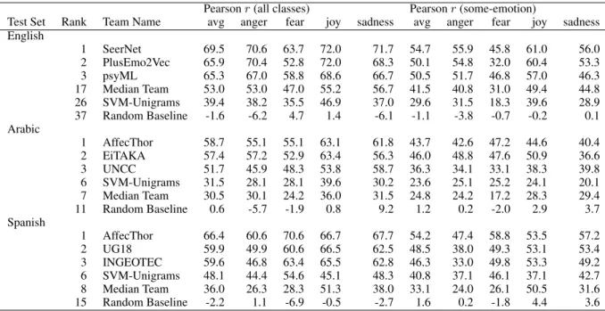
Pearson r (all classes) Pearson r (some-emotion)
Test Set Rank Team Name avg anger fear joy sadness avg anger fear joy sadness English 1 SeerNet 69.5 70.6 63.7 72.0 71.7 54.7 55.9 45.8 61.0 56.0 2 PlusEmo2Vec 65.9 70.4 52.8 72.0 68.3 50.1 54.8 32.0 60.4 53.3 3 psyML 65.3 67.0 58.8 68.6 66.7 50.5 51.7 46.8 57.0 46.3 17 Median Team 53.0 53.0 47.0 55.2 56.7 41.5 40.8 31.0 49.4 44.8 26 SVM-Unigrams 39.4 38.2 35.5 46.9 37.0 29.6 31.5 18.3 39.6 28.9 37 Random Baseline -1.6 -6.2 4.7 1.4 -6.1 -1.1 -3.8 -0.7 -0.2 0.1 Arabic 1 AffecThor 58.7 55.1 55.1 63.1 61.8 43.7 42.6 47.2 44.6 40.4 2 EiTAKA 57.4 57.2 52.9 63.4 56.3 46.0 48.8 47.6 50.9 36.6 3 UNCC 51.7 45.9 48.3 53.8 58.7 36.3 34.1 33.1 38.3 39.8 6 SVM-Unigrams 31.5 28.1 28.1 39.6 30.2 23.6 25.1 25.2 24.1 20.1 7 Median Team 30.5 30.1 24.2 36.0 31.5 24.8 24.2 17.2 28.3 29.4 11 Random Baseline 0.6 -5.7 -1.9 0.8 9.2 1.2 0.2 -2.0 2.9 3.7 Spanish 1 AffecThor 66.4 60.6 70.6 66.7 67.7 54.2 47.4 58.8 53.5 57.2 2 UG18 59.9 49.9 60.6 66.5 62.5 48.5 38.0 49.3 53.1 53.4 3 INGEOTEC 59.6 46.8 63.4 65.5 62.8 46.3 33.0 49.8 53.3 49.2 6 SVM-Unigrams 48.1 44.4 54.6 45.1 48.3 40.8 37.1 46.1 37.1 42.7 8 Median Team 36.0 26.3 28.3 51.3 38.0 33.1 24.0 26.1 50.5 31.6 15 Random Baseline -2.2 1.1 -6.9 -0.5 -2.7 1.6 0.2 -1.8 4.4 3.6
Table 8: Task 2 emotion intensity ordinal classification (EI-oc): Results.
Rank Team Name r(all) r(0.5-1) English 1 SeerNet 87.3 69.7 2 TCS Research 86.1 68.0 3 PlusEmo2Vec 86.0 69.1 18 Median Team 78.4 59.1 31 SVM-Unigrams 58.5 44.9 35 Random Baseline 3.1 1.2 Arabic 1 EiTAKA 82.8 57.8 2 AffecThor 81.6 59.7 3 EMA 80.4 57.6 6 Median Team 72.0 36.2 9 SVM-Unigrams 57.1 42.3 13 Random Baseline -5.2 2.2 Spanish 1 AffecThor 79.5 65.9 2 Amobee 77.0 64.2 3 ELiRF-UPV 74.2 57.1 6 Median Team 60.9 50.9 9 SVM-Unigrams 57.4 51.5 13 Random Baseline -2.3 2.3
Table 9: Task 3 valence regression (V-reg): Results.
High-Ranking Arabic Systems: Top teams trained their systems using deep learning tech-niques, such as CNN, LSTM and Bi-LSTM (Af-fecThor, EiTAKA, UNCC). Traditional machine learning approaches, such as Logistic Regression, Ridge Regression, Random Forest and SVC/SVM, were also employed (EMA, INGEOTEC, PARTNA, Tw-StAR). Many teams relied on Arabic pre-processing and normalization techniques in an attempt to decrease the sparsity due to mor-phological complexity in the Arabic language. EMA applied stemming and lemmatization us-ing MADAMIRA (a morphological analysis and
Rank Team Name r(all) r(some emo) English 1 SeerNet 83.6 88.4 2 PlusEmo2Vec 83.3 87.8 3 Amobee 81.3 86.5 18 Median Team 68.2 75.4 24 SVM-Unigrams 50.9 56.0 36 Random Baseline -1.0 -1.2 Arabic 1 EiTAKA 80.9 84.7 2 AffecThor 75.2 79.2 3 INGEOTEC 74.9 78.9 7 Median Team 55.2 59.6 8 SVM-Unigrams 47.1 50.5 14 Random Baseline 1.1 0.9 Spanish 1 Amobee 76.5 80.4 2 AffecThor 75.6 79.2 3 ELiRF-UPV 72.9 76.5 6 Median Team 55.6 59.1 8 SVM-Unigrams 41.8 46.1 13 Random Baseline -4.2 -4.3
Table 10: Task 4 valence ord. classifn. (V-oc): Results.
disambiguation tool for Arabic), while TwStar and PARTNA used stemmer designed for handling tweets. In addition, top systems applied addi-tional pre-processing, such as dropping punctua-tions, menpunctua-tions, stop words, and hashtag symbols. Many teams (e.g., AffecThor, EiTAKA and EMA) utilized Arabic sentiment lexicons (Mo-hammad et al., 2016; Badaro et al., 2014). Some teams (e.g., EMA) used Arabic translations of the NRC Emotion Lexicon (Mohammad and Turney, 2013). Pre-trained Arabic word embeddings (AraVec) generated from a large set of tweets were also used as additional input features by
EMA and UNCC. AffecThor collected 4.4 million Arabic tweets to train their own word embeddings. Traditional machine learning algorithms (Random Forest, SVR and Ridge regression) used by EMA obtained results rivaling those obtained by deep learning approaches.
High-Ranking Spanish Systems: Convolutional neural networks and recurrent neural networks with gated units such as LSTM and GRU were em-ployed by the winning Spanish teams (AffecThor, Amobee, ELIRF-UPV, UG18). Word embeddings trained from Spanish tweets, such as the ones pro-vided by Rothe et al. (2016), were used as the basis for training deep learning models. They were also employed as features for more traditional learning schemes such as SVMs (UG18). Spanish Affec-tive Lexicons such as the Spanish Emotion Lexi-con (SEL) (Sidorov et al., 2012) and ML-SentiCon (Cruz et al., 2014) were also used to build the fea-ture space (UWB, SINAI). Translation was used in two different ways: 1) automatic translation of En-glish affective lexicons into Spanish (SINAI), and 2): training set augmentation via automatic trans-lation of English tweets (Amobee, UG18).
6.2 Summary
In the standard deep learning or representation learning approach, data representations (tweets in our case) are jointly trained for the task at hand via neural networks with convolution or recurrent lay-ers (LeCun et al., 2015). The claim is that this can lead to more robust representations than relying on manually-engineered features. In contrast, here, most of the top-performing systems employed manually-engineered representations for tweets. These representations combine trained representa-tions, models trained on distant supervision cor-pora, and unsupervised word and sentence embed-dings, with manually-engineered features, such as features derived from affect lexicons. This shows that despite being rather powerful, representation learning can benefit from working in tandem with task-specific features. For emotion intensity tasks, lexicons such as the Affect Intensity Lexicon (Mo-hammad, 2018b) that provide intensity scores are particularly helpful. Similarly, tasks on valence, arousal, and dominance can benefit from lexicons such as ANEW (Bradley and Lang, 1999) and the newly created NRC Valence-Arousal-Dominance Lexicon (Mohammad, 2018a), which has entries for about 20,000 English terms.
micro macro
Rank Team Name acc. F1 F1
English 1 NTUA-SLP 58.8 70.1 52.8 2 TCS Research 58.2 69.3 53.0 3 PlusEmo2Vec 57.6 69.2 49.7 17 Median Team 47.1 59.9 46.4 21 SVM-Unigrams 44.2 57.0 44.3 28 Random Baseline 18.5 30.7 28.5 Arabic 1 EMA 48.9 61.8 46.1 2 PARTNA 48.4 60.8 47.5 3 Tw-StAR 46.5 59.7 44.6 6 SVM-Unigrams 38.0 51.6 38.4 7 Median Team 25.4 37.9 25.0 9 Random Baseline 17.7 29.4 27.5 Spanish 1 MILAB SNU 46.9 55.8 40.7 2 ELiRF-UPV 45.8 53.5 44.0 3 Tw-StAR 43.8 52.0 39.2 4 SVM-Unigrams 39.3 47.8 38.2 7 Median Team 16.7 27.5 18.7 8 Random Baseline 13.4 22.8 21.3
Table 11: Task 5 emotion classification (E-c): Results.
7 Examining Gender and Race Bias in Sentiment Analysis Systems
Automatic systems can benefit society by pro-moting equity, diversity, and fairness. Nonethe-less, as machine learning systems become more human-like in their predictions, they are inadver-tently accentuating and perpetuating inappropriate human biases. Examples include, loan eligibility and crime recidivism prediction systems that nega-tively assess people belonging to a certain pin/zip code (which may disproportionately impact peo-ple of a certain race) (Chouldechova, 2017), and resum´e sorting systems that believe that men are more qualified to be programmers than women (Bolukbasi et al., 2016). Similarly, sentiment and emotion analysis systems can also perpetuate and accentuate inappropriate human biases, e.g., sys-tems that consider utterances from one race or gender to be less positive simply because of their race or gender, or customer support systems that prioritize a call from an angry male user over a call from the equally angry female user.
Discrimination-aware data mining focuses on measuring discrimination in data (Zliobaite, 2015; Pedreshi et al., 2008; Hajian and Domingo-Ferrer, 2013). In that spirit, we carried out an analysis of the systems’ outputs for biases towards cer-tain races and genders. In particular, we wanted to test a hypothesis that a system should equally rate the intensity of the emotion expressed by two sentences that differ only in the gender/race of a person mentioned. Note that here the term system
refers to the combination of a machine learning ar-chitecture trained on a labeled dataset, and possi-bly using additional language resources. The bias can originate from any or several of these parts.
We used Equity Evaluation Corpus (EEC), a re-cently created dataset of 8,640 English sentences carefully chosen to tease out gender and race bi-ases (Kiritchenko and Mohammad, 2018). We used the EEC as a supplementary test set in the EI-reg and V-reg English tasks. Specifically, we compare emotion and sentiment intensity scores that the systems predict on pairs of sentences in the EEC that differ only in one word corresponding to race or gender (e.g., ‘This man made me feel an-gry’ vs. ‘This woman made me feel anan-gry’). Com-plete details on how the EEC was created, its con-stituent sentences, and the analysis of automatic systems for race and gender bias is available in Kiritchenko and Mohammad (2018); we summa-rize the key results below.
Despite the work we describe here and that pro-posed by others, it should be noted that mecha-nisms to detect bias can often be circumvented. Nonetheless, as developers of sentiment analysis systems, and NLP systems more broadly, we can-not absolve ourselves of the ethical implications of the systems we build. Thus, the Equity Evalu-ation Corpus is not meant to be a catch-all for all inappropriate biases, but rather just one of the sev-eral ways by which we can examine the fairness of sentiment analysis systems. The EEC corpus is freely available so that both developers and users can use it, and build on it.18
7.1 Methodology
The race and gender bias evaluation was carried out on the EI-reg and V-reg predictions of 219 automatic systems (by 50 teams) on the EEC sentences. The EEC sentences were created from simple templates such as ‘<noun phrase> feels devastated’, where <noun phrase> is replaced with one of the following:
• common African American (AA) female and male first names,
• common European American (EA) female and male first names,
• noun phrases referring to females and males, such as ‘my daughter’ and ‘my son’.
Notably, one can derive pairs of sentences from the EEC such that they differ only in one phrase
cor-18http://saifmohammad.com/WebPages/Biases-SA.html
responding to gender or race (e.g., ‘My daughter feels devastated’ and ‘My son feels devastated’). For the full lists of names, noun phrases, and sen-tence templates see (Kiritchenko and Mohammad, 2018). In total, 1,584 pairs of scores were com-pared for gender and 144 pairs of scores were compared for race.
For each submission, we performed the paired two sample t-test to determine whether the mean difference between the two sets of scores (across the two races and across the two genders) is signif-icant. We set the significance level to 0.05. How-ever, since we performed 438 assessments (219 submissions evaluated for biases in both gender and race), we applied Bonferroni correction. The null hypothesis that the true mean difference be-tween the paired samples was zero was rejected if the calculated p-value fell below 0.05/438. 7.2 Results
7.2.1 Gender Bias Results
Individual submission results were communicated to the participants. Here, we present the summary results across all the teams. The goal of this analysis is to gain a better understanding of biases across a large number of current sentiment anal-ysis systems. Thus, we partition the submissions into three groups according to the bias they show: • F = M: submissions that showed no statistically significant difference in intensity scores pre-dicted for corresponding female and male noun phrase sentences,
• F↑–M↓: submissions that consistently gave higher scores for sentences with female noun phrases than for corresponding sentences with male noun phrases,
• F↓–M↑: submissions that consistently gave lower scores for sentences with female noun phrases than for corresponding sentences with male noun phrases,
Table 12 shows the number of submissions in each group. If all the systems are unbiased, then the number of submissions for the group F = M would be the maximum, and the number of submissions in all other groups would be zero.
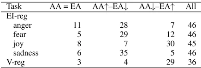
Observe that on the four emotion intensity pre-diction tasks, only about 12 of the 46 submissions (about 25% of the submissions) showed no sta-tistically significant score difference. On the va-lence prediction task, only 5 of the 36 submissions (14% of the submissions) showed no statistically
Task F = M F↑–M↓ F↓–M↑ all EI-reg anger 12 21 13 46 fear 11 12 23 46 joy 12 25 8 45 sadness 12 18 16 46 V-reg 5 22 9 36
Table 12: Analysis of gender bias: The number of submissions in each of the three bias groups.
significant score difference. Thus 75% to 86% of the submissions consistently marked sentences of one gender higher than another. When predict-ing anger, joy, or valence, the number of systems consistently giving higher scores to sentences with female noun phrases (21–25) is markedly higher than the number of systems giving higher scores to sentences with male noun phrases (8–13). (Re-call that higher valence means more positive sen-timent.)
In contrast, on the fear task, most submissions tended to assign higher scores to sentences with male noun phrases (23) as compared to the num-ber of systems giving higher scores to sentences with female noun phrases (12). When predicting sadness, the number of submissions that mostly assigned higher scores to sentences with female noun phrases (18) is close to the number of submissions that mostly assigned higher scores to sentences with male noun phrases (16).
7.2.2 Race Bias Results
We did a similar analysis as for gender, for race. For each submission on each task, we calculated the difference between the average predicted score on the set of sentences with African American (AA) names and the average predicted score on the set of sentences with European American (EA) names. Then, we aggregated the results over all such sentence pairs in the EEC.
Table 13 shows the results. The table has the same form and structure as the gender result ta-ble. Observe that the number of submissions with no statistically significant score difference for sen-tences pertaining to the two races is about 5–11 (about 11% to 24%) for the four emotions and 3 (about 8%) for valence. These numbers are even lower than what was found for gender.
The majority of the systems assigned higher scores to sentences with African American names on the tasks of anger, fear, and sadness intensity prediction. On the joy and valence tasks, most submissions tended to assign higher scores to
sen-Task AA = EA AA↑–EA↓ AA↓–EA↑ All
EI-reg anger 11 28 7 46 fear 5 29 12 46 joy 8 7 30 45 sadness 6 35 5 46 V-reg 3 4 29 36
Table 13: Analysis of race bias: The number of sub-missions in each of the three bias groups.
tences with European American names.
We found the score differences across genders and across races to be somewhat small (< 0.03 in magnitude, which is 3% of the 0 to 1 score range). However, what impact a consistent bias, even with a magnitude < 3%, might have in downstream ap-plications merits further investigation.
8 Summary
We organized the SemEval-2018 Task 1: Affect in Tweets, which included five subtasks on infer-ring the affectual state of a person from their tweet. For each task, we provided training, development, and test datasets for English, Arabic, and Span-ish tweets. This involved creating a new Affect in Tweets dataset of more than 22,000 tweets such that subsets are annotated for a number of emotion dimensions. For each emotion dimension, we an-notated the data not just for coarse classes (such as anger or no anger) but also for fine-grained real-valued scores indicating the intensity of emo-tion. We used Best–Worst Scaling to obtain fine-grained real-valued intensity scores and showed that the annotations are reliable (split-half reliabil-ity scores > 0.8).
Seventy-five teams made 319 submissions to the fifteen task–language pairs. Most of the top-performing teams relied on both deep neural net-work representations of tweets (sentence embed-dings) as well as features derived from existing sentiment and emotion lexicons. Apart from the usual evaluations for the quality of predictions, we also examined 219 EI-reg and V-reg English submissions for bias towards particular races and genders using the Equity Evaluation Corpus. We found that a majority of the systems consistently provided slightly higher scores for one race or gen-der. All of the data is made freely available.19
References
Gilbert Badaro, Ramy Baly, Hazem M. Hajj, Nizar Habash, and Wassim El-Hajj. 2014. A large scale arabic sentiment lexicon for arabic opinion mining. In Proceedings of the EMNLP 2014 Workshop on Arabic Natural Language Processing, pages 165– 173, Doha, Qatar.
Tolga Bolukbasi, Kai-Wei Chang, James Y Zou, Venkatesh Saligrama, and Adam T Kalai. 2016. Man is to computer programmer as woman is to homemaker? debiasing word embeddings. In Pro-ceedings of the Annual Conference on Neural In-formation Processing Systems (NIPS), pages 4349– 4357.
Margaret M Bradley and Peter J Lang. 1999. Affective norms for English words (ANEW): Instruction man-ual and affective ratings. Technical report, The Cen-ter for Research in Psychophysiology, University of Florida.
Alexandra Chouldechova. 2017. Fair prediction with disparate impact: A study of bias in recidivism pre-diction instruments. Big data, 5(2):153–163. LJ Cronbach. 1946. A case study of the splithalf
reli-ability coefficient. Journal of educational psychol-ogy, 37(8):473.
Ferm´ın L Cruz, Jos´e A Troyan, Beatriz Pontes, and F Javier Ortega. 2014. Ml-senticon: Un lexic´on multiling¨ue de polaridades sem´anticas a nivel de lemas. Procesamiento del Lenguaje Natural, (53). Paul Ekman. 1992. An argument for basic emotions.
Cognition and Emotion, 6(3):169–200.
Bjarke Felbo, Alan Mislove, Anders Søgaard, Iyad Rahwan, and Sune Lehmann. 2017. Using millions of emoji occurrences to learn any-domain represen-tations for detecting sentiment, emotion and sar-casm. In Proceedings of the 2017 Conference on Empirical Methods in Natural Language Process-ing, 2017, Copenhagen, Denmark, September 9-11, 2017, pages 1615–1625.
T. N. Flynn and A. A. J. Marley. 2014. Best-worst scal-ing: theory and methods. In Stephane Hess and An-drew Daly, editors, Handbook of Choice Modelling, pages 178–201. Edward Elgar Publishing.
Nico H Frijda. 1988. The laws of emotion. American psychologist, 43(5):349.
Sara Hajian and Josep Domingo-Ferrer. 2013. A methodology for direct and indirect discrimination prevention in data mining. IEEE Transactions on Knowledge and Data Engineering, 25(7):1445– 1459.
Minqing Hu and Bing Liu. 2004. Mining and summa-rizing customer reviews. In Proceedings of the tenth ACM SIGKDD international conference on Knowl-edge discovery and data mining, pages 168–177, New York, NY, USA. ACM.
Svetlana Kiritchenko and Saif M. Mohammad. 2016. Capturing reliable fine-grained sentiment associa-tions by crowdsourcing and best–worst scaling. In Proceedings of The 15th Annual Conference of the North American Chapter of the Association for Computational Linguistics: Human Language Tech-nologies (NAACL), San Diego, California.
Svetlana Kiritchenko and Saif M. Mohammad. 2017. Best-worst scaling more reliable than rating scales: A case study on sentiment intensity annotation. In Proceedings of The Annual Meeting of the Associa-tion for ComputaAssocia-tional Linguistics (ACL), Vancou-ver, Canada.
Svetlana Kiritchenko and Saif M. Mohammad. 2018. Examining gender and race bias in two hundred sen-timent analysis systems. In Proceedings of the 7th Joint Conference on Lexical and Computational Se-mantics (*SEM).
Svetlana Kiritchenko, Xiaodan Zhu, and Saif M. Mo-hammad. 2014. Sentiment analysis of short in-formal texts. Journal of Artificial Intelligence Re-search, 50:723–762.
Ryan Kiros, Yukun Zhu, Ruslan R Salakhutdinov, Richard Zemel, Raquel Urtasun, Antonio Torralba, and Sanja Fidler. 2015. Skip-thought vectors. In Advances in neural information processing systems, pages 3294–3302.
G Frederic Kuder and Marion W Richardson. 1937. The theory of the estimation of test reliability. Psy-chometrika, 2(3):151–160.
Yann LeCun, Yoshua Bengio, and Geoffrey Hinton. 2015. Deep learning. Nature, 521(7553):436. Jordan J. Louviere. 1991. Best-worst scaling: A model
for the largest difference judgments. Working Paper. Saif Mohammad, Mohammad Salameh, and Svetlana Kiritchenko. 2016. Sentiment lexicons for arabic social media. In Proceedings of the Tenth Interna-tional Conference on Language Resources and Eval-uation (LREC 2016), Paris, France. European Lan-guage Resources Association (ELRA).
Saif M. Mohammad. 2016. Sentiment analysis: De-tecting valence, emotions, and other affectual states from text. In Herb Meiselman, editor, Emotion Mea-surement. Elsevier.
Saif M. Mohammad. 2018a. Obtaining reliable hu-man ratings of valence, arousal, and dominance for 20,000 english words. In Proceedings of The An-nual Meeting of the Association for Computational Linguistics (ACL), Melbourne, Australia.
Saif M. Mohammad. 2018b. Word affect intensities. In Proceedings of the 11th Edition of the Language Re-sources and Evaluation Conference (LREC-2018), Miyazaki, Japan.
Saif M. Mohammad and Felipe Bravo-Marquez. 2017. WASSA-2017 shared task on emotion intensity. In Proceedings of the Workshop on Computational Ap-proaches to Subjectivity, Sentiment and Social Me-dia Analysis (WASSA), Copenhagen, Denmark. Saif M. Mohammad and Svetlana Kiritchenko. 2018.
Understanding emotions: A dataset of tweets to study interactions between affect categories. In Pro-ceedings of the 11th Edition of the Language Re-sources and Evaluation Conference (LREC-2018), Miyazaki, Japan.
Saif M. Mohammad, Parinaz Sobhani, and Svetlana Kiritchenko. 2017. Stance and sentiment in tweets. Special Section of the ACM Transactions on Inter-net Technology on Argumentation in Social Media, 17(3).
Saif M. Mohammad and Peter D. Turney. 2013. Crowdsourcing a word–emotion association lexicon. Computational Intelligence, 29(3):436–465. Finn ˚Arup Nielsen. 2011. A new ANEW: Evaluation
of a word list for sentiment analysis in microblogs. In Proceedings of the ESWC Workshop on ’Mak-ing Sense of Microposts’: Big th’Mak-ings come in small packages, pages 93–98, Heraklion, Crete.
Bryan Orme. 2009. Maxdiff analysis: Simple count-ing, individual-level logit, and HB. Sawtooth Soft-ware, Inc.
Raquel Mochales Palau and Marie-Francine Moens. 2009. Argumentation mining: the detection, clas-sification and structure of arguments in text. In Pro-ceedings of the 12th international conference on ar-tificial intelligence and law, pages 98–107.
W Parrot. 2001. Emotions in Social Psychology. Psy-chology Press.
Dino Pedreshi, Salvatore Ruggieri, and Franco Turini. 2008. Discrimination-aware data mining. In Pro-ceedings of the 14th ACM SIGKDD International Conference on Knowledge Discovery and Data Min-ing, pages 560–568.
Robert Plutchik. 1980. A general psychoevolutionary theory of emotion. Emotion: Theory, research, and experience, 1(3):3–33.
Alec Radford, Rafal Jozefowicz, and Ilya Sutskever. 2017. Learning to generate reviews and discovering sentiment. arXiv preprint arXiv:1704.01444. Sascha Rothe, Sebastian Ebert, and Hinrich Sch¨utze.
2016. Ultradense word embeddings by orthogonal transformation. In HLT-NAACL.
James A Russell. 1980. A circumplex model of af-fect. Journal of personality and social psychology, 39(6):1161.
James A Russell. 2003. Core affect and the psycholog-ical construction of emotion. Psychologpsycholog-ical review, 110(1):145.
Grigori Sidorov, Sabino Miranda-Jim´enez, Francisco Viveros-Jim´enez, Alexander Gelbukh, No´e Castro-S´anchez, Francisco Vel´asquez, Ismael D´ıaz-Rangel, Sergio Su´arez-Guerra, Alejandro Trevi˜no, and Juan Gordon. 2012. Empirical study of machine learn-ing based approach for opinion minlearn-ing in tweets. In Mexican international conference on Artificial intel-ligence, pages 1–14. Springer.
Michael Wojatzki, Saif M. Mohammad, Torsten Zesch, and Svetlana Kiritchenko. 2018. Quantifying quali-tative data for understanding controversial issues. In Proceedings of the 11th Edition of the Language Re-sources and Evaluation Conference (LREC-2018), Miyazaki, Japan.
Indre Zliobaite. 2015. A survey on measuring indirect discrimination in machine learning. arXiv preprint arXiv:1511.00148.
Appendix
Table 14 shows the summary details of the annotations done for the SemEval-2018 Affect in Tweets dataset. Figure 5 shows the histograms of the EI-reg tweets in the anger, joy, sadness, and fear datasets. The tweets are grouped into bins of scores 0–0.05, 0.05–0.1, and so on until 0.95–1. The colors for the bins correspond to their ordinal classes: no emotion, low emotion, moderate emotion, and high emotion. The ordinal classes were determined from the EI-oc manual annotations.
Supplementary Material: The supplementary pdf associated with this paper includes longer ver-sions of tables included in this paper. Tables 1 to 15 in the supplementary pdf show result tables that include the scores of each of the 319 systems participating in the tasks. Table 16 in the supple-mentary pdf shows the annotator agreement for each of the twelve classes, for each of the three languages, in the Multi-label Emotion Classifica-tion (E-c) Dataset. We observe that the Fleiss’ κ scores are markedly higher for the frequently oc-curring four basic emotions (joy, sadness, fear, and anger), and lower for the less frequent emotions. (Frequencies for the emotions are shown in Table 2.) Also, agreement is low for the neutral class. This is not surprising because the boundary be-tween neutral (or no emotion) and slight emotion is fuzzy. This means that often at least one or two annotators indicate that the person is feeling some joy or some sadness, even if most others indicate that the person is not feeling any emotion.
Figure 5:Emotion intensity score (EI-reg) and ordinal class (EI-oc) distributions for the four basic emotions in the SemEval-2018 AIT development and test sets combined. The distribution is similar for the training set (annotated in earlier work).
Dataset Scheme Location Item #Items #Annotators MAI #Q/Item #Annotat.
English
E-c categorical World tweet 11,090 303 7 2 174,356
EI-reg
anger BWS USA 4-tuple of tweets 2,780 168 4 2 27,046
fear BWS USA 4-tuple of tweets 2,750 220 4 2 26,908
joy BWS USA 4-tuple of tweets 2,790 132 4 2 26,676
sadness BWS USA 4-tuple of tweets 2,744 118 4 2 26,260
V-reg BWS USA 4-tuple of tweets 5,134 175 4 2 49,856
Total 331,102
Arabic
E-c categorical World tweet 4,400 175 7 1 36,274
EI-reg
anger BWS World 4-tuple of tweets 2,800 221 4 2 25,960
fear BWS World 4-tuple of tweets 2,800 197 4 2 25,872
joy BWS World 4-tuple of tweets 2,800 133 4 2 24,690
sadness BWS World 4-tuple of tweets 2,800 177 4 2 25,834
V-reg BWS World 4-tuple of tweets 3,600 239 4 2 36,824
Total 175,454
Spanish
E-c categorical World tweet 7,182 160 7 1 56,274
EI-reg
anger BWS World 4-tuple of tweets 3,972 157 3 2 27,456
fear BWS World 4-tuple of tweets 3,972 388 3 2 29,530
joy BWS World 4-tuple of tweets 3,980 323 3 2 28,300
sadness BWS World 4-tuple of tweets 3,982 443 3 2 28,462
V-reg BWS World 4-tuple of tweets 4,886 220 3 2 38,680
Total 208,702
Table 14: Summary details of the current annotations done for the SemEval-2018 Affect in Tweets Dataset. MAI = Median Annotations per Item. Q = annotation questions.