Publisher’s version / Version de l'éditeur:
Vous avez des questions? Nous pouvons vous aider. Pour communiquer directement avec un auteur, consultez la première page de la revue dans laquelle son article a été publié afin de trouver ses coordonnées. Si vous n’arrivez pas à les repérer, communiquez avec nous à [email protected].
Questions? Contact the NRC Publications Archive team at
[email protected]. If you wish to email the authors directly, please see the first page of the publication for their contact information.
https://publications-cnrc.canada.ca/fra/droits
L’accès à ce site Web et l’utilisation de son contenu sont assujettis aux conditions présentées dans le site LISEZ CES CONDITIONS ATTENTIVEMENT AVANT D’UTILISER CE SITE WEB.
New Journal of Physics, 21, 8, 2019-09-28
READ THESE TERMS AND CONDITIONS CAREFULLY BEFORE USING THIS WEBSITE.
https://nrc-publications.canada.ca/eng/copyright
NRC Publications Archive Record / Notice des Archives des publications du CNRC :
https://nrc-publications.canada.ca/eng/view/object/?id=9a856c70-f130-439e-b491-a9b26e54597b
https://publications-cnrc.canada.ca/fra/voir/objet/?id=9a856c70-f130-439e-b491-a9b26e54597b
Archives des publications du CNRC
This publication could be one of several versions: author’s original, accepted manuscript or the publisher’s version. / La version de cette publication peut être l’une des suivantes : la version prépublication de l’auteur, la version acceptée du manuscrit ou la version de l’éditeur.
For the publisher’s version, please access the DOI link below./ Pour consulter la version de l’éditeur, utilisez le lien DOI ci-dessous.
https://doi.org/10.1088/1367-2630/ab3871
Access and use of this website and the material on it are subject to the Terms and Conditions set forth at
Robust optical clock transitions in trapped ions using dynamical
decoupling
Aharon, Nati; Spethmann, Nicolas; Leroux, Ian D.; Schmidt, Piet O.; Retzker,
Alex
PAPER • OPEN ACCESS
Robust optical clock transitions in trapped ions
using dynamical decoupling
To cite this article: Nati Aharon et al 2019 New J. Phys. 21 083040
View the article online for updates and enhancements.
Recent citations
Sub-kelvin temperature management in ion traps for optical clocks
T. Nordmann et al
-Coherent Suppression of Tensor Frequency Shifts through Magnetic Field Rotation
R. Lange et al
-Precision Measurements of the Ba+138 6sS21/25dD25/2 Clock Transition
K. J. Arnold et al
PAPER
Robust optical clock transitions in trapped ions using dynamical
decoupling
Nati Aharon1
, Nicolas Spethmann2
, Ian D Leroux2,3
, Piet O Schmidt2,4
and Alex Retzker1
1 Racah Institute of Physics, The Hebrew University of Jerusalem, Jerusalem 91904, Givat Ram, Israel
2 QUEST Institute for Experimental Quantum Metrology, Physikalisch-Technische Bundesanstalt, D-38116 Braunschweig, Germany 3 National Research Council Canada, Ottawa, Ontario, K1A 0R6, Canada
4 Institut für Quantenoptik, Leibniz Universität Hannover, D-30167 Hannover, Germany E-mail:[email protected]
Keywords: optical clocks, multi-ion optical clocks, dynamical decoupling
Abstract
We present a novel method for engineering an optical clock transition that is robust against external
field
fluctuations and is able to overcome limits resulting from field inhomogeneities. The technique is based on
the application of continuous driving
fields to form a pair of dressed states essentially free of all relevant
shifts. Specifically, the clock transition is robust to magnetic field shifts, quadrupole and other tensor shifts,
and amplitude
fluctuations of the driving fields. The scheme is applicable to either a single ion or an
ensemble of ions, and is relevant for several types of ions, such as Ca
40 +, Sr
88 +,
138Ba
+and
176Lu
+. Taking a
spherically symmetric Coulomb crystal formed by 400 Ca
40 +ions as an example, we show through
numerical simulations that the inhomogeneous linewidth of tens of Hertz in such a crystal together with
linear Zeeman shifts of order 10MHz are reduced to form a linewidth of around 1Hz. We estimate a
two-order-of-magnitude reduction in averaging time compared to state-of-the art single ion frequency
references, assuming a probe laser fractional instability of 10
-15. Furthermore, a statistical uncertainty
reaching 2.9×10
−16in 1s is estimated for a cascaded clock scheme in which the dynamically decoupled
Coulomb crystal clock stabilizes the interrogation laser for an Al
27 +clock.
1. Introduction
Optical clocks based on neutral atoms trapped in optical lattices and single trapped ions have reached estimated systematic uncertainties of a few parts in 10−18[1–4] or even below [5]. Taking advantage of these record
uncertainties for applications ranging from relativistic geodesy[6–9] over fundamental physics [10–12] to
frequency metrology[13–17] requires achieving statistical measurement uncertainties of the same level within
practical averaging timesτ (given in seconds). This has been achieved with single-ensemble optical lattice clocks in self-comparison experiments up to a level of 1.6´10-16 t[18] and by implementing an effectively
dead-time-free clock consisting of two independent clocks probed in an interleaved fashion[19,20], reaching a
statistical uncertainty in the range of 5´10-17 t. In contrast to neutral atom lattice clocks, which are
typically probed with hundreds to thousands of atoms, single ion clocks are currently limited in their statistical uncertainty by quantum projection noise[21] to levels of a few parts in 10-15 t[3,22,23]. The statistical
uncertainty can be improved by probing for longer times, ultimately limited by the excited clock state lifetime or the laser coherence time[24,25]. Alternatively, the number of probed ions can be increased.
Recently, multi-ion clock schemes have been proposed to address this issue[26–29]. However, several
challenges have to be overcome to maintain and transfer the small and very well characterizable systematic shifts achievable with single trapped ions to larger ion crystals. The oscillating rffield in Paul traps results in ac Stark and second order Doppler shifts through micromotion[30–32]. Furthermore, electric field gradients from the
trappingfields and the surrounding ions couple to atomic quadrupole moments, resulting in an electric quadrupole shift(QPS). The effects of micromotion can be avoided by trapping strings of ions in a precision-machined linear Paul trap with negligible excess micromotion from trap imperfections[28,33]. The QPS in such OPEN ACCESS
RECEIVED 3 July 2019 ACCEPTED FOR PUBLICATION 5 August 2019 PUBLISHED 28 August 2019 Original content from this work may be used under the terms of theCreative Commons Attribution 3.0 licence.
Any further distribution of this work must maintain attribution to the author(s) and the title of the work, journal citation and DOI.
chains can be avoided by choosing an ion species with negligible differential electric quadrupole moment between the clock states, such asIn+orAl+, or by employing ring traps in which the QPS is the same for all ions [29]. A high-accuracy multi-ion clock based on ion chains containing on the order of tens of ions in a linear
quadrupole trap has been proposed and is expected to achieve trap-induced fractional systematic uncertainties at the 10−19level[26].
An alternative approach based on large 3d Coulomb crystals of ions has been theoretically investigated[27]
for ion species for which the micromotion-induced Doppler shift and the scalar ac Stark shift, both driven by the rf trappingfield, can be made to cancel at a ‘magic’ rf drive frequency [30]. This cancellation has been employed
for singleSr+[34], single Ca+[35], and is currently being investigated forLu+[27,36,37]. However, electronic
states with J>1/2 are subject to rank 2 tensor shifts, such as rf electric field-induced tensor ac Stark shift (TASS) and QPS[30,32]. For 3d Coulomb crystals with tens up to several hundreds of ions, this results in
position-dependent shifts, since the electricfield environment of the ions differ. It has been proposed to reduce this inhomogeneous broadening across the ion crystal by employing a spherical ion crystal to minimize the QPS and by adding a compensating laserfield for the TASS [27], or by operating at a judiciously chosen
magnetic-field-insensitive point[37] for ions with hyperfine structure.
Achieving insensitivity of atomic energy levels to externalfield fluctuations has been theoretically investigated using pulsed or continuous dynamical decoupling(CDD) [38–48]. Such schemes have been
experimentally implemented in various systems ranging from NV centers and solid state spin systems[49–57] to
neutral atoms[58] and trapped ions [59–64].
CDD or dressed-state engineering in the context of clocks has been proposed for linear Zeeman shift cancellation in neutral atom clocks through rf dressing of Zeeman substates in a regime where the drive Rabi frequency is larger than the drive frequency[45]. However, this scheme is unable to cancel tensorial shifts, such
as the QPS or TASS. In a similar approach, magneticfield noise suppression up to second order in radio-frequency clocks via weak rf dressing has been proposed[46] and experimentally implemented to engineer
synthetic clock states for rf spectroscopy in ultra-cold rubidium[65,66].
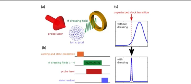
Here, we show through numerical simulations that CDD using four rf frequencies significantly suppresses all relevant homogeneous(linear Zeeman) and inhomogeneous (micromotion-induced second order Doppler, QPS, scalar and tensor ac Stark) frequency shifts on an optical clock transition for an ion crystal containing 400 ions. We note that the scheme in principle works for any ion number and crystal size. We demonstrate the basic principle, which is illustrated infigure1, on the S2
1 2«2D5 2clock transition in Ca40 +, but the scheme is directly applicable
to other systems as well. It therefore allows the operation of a multi-ion clock[26] using ion species whose clock
transitions have a non-vanishing differential electric quadrupole moment. One of the many possible applications of such a multi-ion frequency reference is the phase stabilization of a probe laser for a single ion clock to allow near-lifetime-limited probe times and correspondingly reduced statistical uncertainties[24,25].
The paper is organized as follows. In section2wefirst show how robustness to QPS and TASS can be achieved by the application of a single continuous detuned drivingfield. The discussion of only one driving field gives a simple and intuitive understanding of our approach. In section3we extend the discussion to the full CDD scheme employing four drivingfields for the construction of a robust optical clock transition. For simplicity and
Figure 1. Schematic representation of the setup.(a) The ion crystal is probed while it is being manipulated by the rf dressing fields. (b) Schematic representation of the sequence considered in this scheme. (c) Illustration of the robust clock transition. While the unperturbed clock transition is subject to magnetic shifts, quadrupole shifts, and tensor shifts, the dressingfields substantially mitigate these shifts and result in a robust clock transition.
clarity in the discussion we ignore effects of the counter-rotating terms of the drivingfields by assuming the rotating-wave-approximation(RWA), as well as the cross-driving effects (for example, the effect of the S2
1 2
drivingfield on the D2
5 2states). These two effects are, however, taken into account when numerically
optimizing the driving parameters as well as in the simulations presented. In appendicesC–E, we show in detail how this is achieved by incorporating these effects in the optimization. Then, in section4we consider the implementation of the scheme in the case of a multi-ion crystal clock and analyze the performance of the scheme in terms of the expected statistical uncertainties of the robust optical clock transition. After discussing possible applications in section5, we end with the conclusions in section6.
2. Robustness to tensor shifts
In the absence of hyperfine structure, tensor shifts including the QPS are proportional to QJ m, j=J J( +1)-3mj2
[32], where J is the total angular momentum and mJthe magnetic quantum number. These shifts reduce the
precision of atomic clocks when not suppressed by suitable averaging schemes. Previously employed schemes to suppress the quadrupole shift include averaging the transition frequency over all mJstates, sinceåmJJ=-JQJ m, j=0
[67]. Such an average will also eliminate the linear Zeeman shift, assuming the field does not change between the
frequency measurements contributing to the average. We propose a novel dynamical decoupling scheme in which robustness to this type of shifts is achieved by the application of a detuned drivingfield, mixing all mJstates to form
dressed states with effective QJ m, j= . While the cancellation scheme is general and applies to tensor shifts of0 arbitrary electronic states, we consider in the following the Hamiltonian of the D2
5 2states of e.g.Ca+ions
H=gdmBBSz +gdW1cos[(gdmBB-d1) ]t Sx, ( )1 where gdμBB is the Zeeman splitting due to the static magneticfield B, gdis the gyromagnetic ratio of the D2 5 2
states, Szand Sxare the z and x spin-5/2 matrices,W1is the Rabi frequency of the drivingfield, and δ1is the
detuning. Moving to the interaction picture(IP) with respect to H0=(gdμBB− δ1)Szand taking the RWA
( g( dmBB-d1)W1), results in H S g S 2 , 2 I 1 z d x 1 d = + W ( )
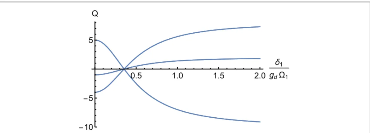
where HIis the Hamiltonian in the IP. Since the bare D2 5 2states have tensor shifts which are proportional to Q5 2, 5 2 = -10, Q5 2, 3 2 = +2, and Q5 2, 1 2 = +8, the tensor shifts of the dressed states(the eigenstates
of HI) are proportional to Q= -5q(d1,W1), +q(d1,W1), +4q(d1,W1), ( )3 with q g g , 8 4 . 4 d d 1 1 1 2 12 12 12 d d d W = - + W + W ( ) ( ) ( ) ( )
Hence, by choosingd = 1 18(gdW1), all of the dressed states have a zero(first order) tensor shift, Q=0
(see figure2). Similarly, for a fixed detuning δ1choosingW =1 8d1 gdresults in a zero tensor shift. This can
also be understood in the lab frame, in which the couplingΩ1drives a rotation among the bare states, averaging
their shifts in time just as in the mJaveraging scheme mentioned above. However, here the averaging takes place
at a rate corresponding to the Rabi frequency rather than the experiment repetition rate, allowing it to suppress much fasterfield fluctuations.
The cancellation of the tensor shift tofirst order can also be understood as follows. The tensor and quadrupole shift operator Qˆ =S2-3Sz2can also be written as Q S S 2S
x2 y2 z2
= +
-ˆ . Moving to a rotated basis (dressed states basis) defined by zcos( )q z+sin( )q x, xcos( )q x-sin( )q z, and y , and neglectingy
purely off-diagonal terms we obtain that Qˆ »Sz2(1-3 cos2( ))q +Sx2(1-3 sin2( ))q +Sy2. Tofirst order
(diagonal terms) we have that Q» S S +S S 2-3 sin2 q +Sz2 1-3 cos2 q ,
+ - - +
ˆ ( )( ( )) ( ( )) where S±=Sx±iSy are the spin ladder operators. Hence tofirst order, the tensor shift vanishes for cos 1
3 q =
( ) , which is analogous to magic-angle spinning in solid-state NMR spectroscopy[68]. The detuned driving field results in dressed
states, which are the eigenstates of equation(2). The rotation to the dressed states basis is given by U=eiqSy,
where cos gd 12 12 1 2 4 q = d d + W ( ) ( ) . For 1 gd 1 8 1 d = ( W)we obtain cos 1 3 q = ( ) .
3. The scheme
Our scheme is based on the application of continuous drivingfields for the construction of a robust optical clock transition. We consider the sub-levels of the S2
1 2and D2 5 2states, the usual clock states in Ca+optical clocks.
Four drivingfields are employed, where two driving fields operate on the S2
1 2states, and two drivingfields
operate on the D2
5 2states. The rf drivingfields continuously drive the bare S2 1 2and D2 5 2states, that is,
continuously couple between the Zeeman sub-levels, which results in the desired robust optical transition of the dressed states. Thefirst driving field of the D2
5 2states mitigates tensor shifts, including the QPS, as shown in the
previous section. However, the D2
5 2states, as well as the S2 1 2states, are still sensitive to the linear Zeeman
shift. Moreover, the D2
5 2states are also sensitive to amplitudefluctuations of the driving field. The purpose of
adding three more drivingfields is to have enough control degrees of freedom that can be tuned such that the suppression of both linear Zeeman shift and amplitudefluctuations of a single (dressed) S2
1 2«2D5 2
transition is achieved. Hence, the driving scheme results in doubly-dressed S2
1 2and D2 5 2states where one
S D
2
1 2« 2 5 2transition(between the doubly-dressed states) is robust to magnetic shifts, quadrupole shifts,
tensor shifts, and driving amplitude shifts caused by amplitudefluctuations of the driving fields (see figure3).
For the D2
5 2( S2 1 2) states, the Rabi frequencies,W , and the detunings,k δk, of thefirst and second driving fields
are denoted by{Ω1,δ1} and {Ω2,δ2} ({Ω3,δ3} and {Ω4,δ4}), respectively. We assume that a static magnetic field
B is applied, which results in the Zeeman splitting of the S2
1 2and D2 5 2states. The rf dressing is based on
magnetic dipole coupling between the Zeeman sub-levels, where the Rabi frequency of a drivingfield is related to
Figure 2. The tensor shift factors Q of the dressed states(equation (3)) as function of the detuning δ1. The tensor shifts vanish for
gd
1 18 1
d = ( W).
Figure 3. Robust multi-ion crystal clock.(a) Typical Zeeman, tensor and quadrupole shifts of the unperturbed clock transition. (b) Two driving fields with a Rabi frequency of ΩS(ΩD) couple the Zeeman substates in the S21 2(2D5 2) manifold, respectively. In our
scheme, we employ multi-frequencyfields for coupling, as discussed in detail in the main text. (c) The double-dressed states. A robust optical transition with a total shift1 Hzand inhomogeneous linewidth∼1 Hz is constructed between the S∣ 2ñand D∣ 4ñstates.
the magnetic dipole moment byW =m Brf
· , where mis the magnetic dipole moment and Brf
is the amplitude vector of the oscillating rffield.
For simplicity and clarity, in the following analysis we neglect the effect of the counter-rotating terms of the drivingfields by assuming the RWA, as well as the cross-driving effects. Both the counter-rotating terms and the cross-drivingfields result in small energy shifts, which are taken into account when optimizing the driving parameters. This, however, does not change the overall physical picture, and results only in small variations of the optimal driving parameters. In appendicesC–Ewe show how this can be done by incorporating these effects in the following optimization.
Similar to the derivation in section2, by moving to thefirst IP with respect to the frequencies of the first drivingfields we obtain the dressed states, which are the eigenstates of
H S g S s g s 2 2 , 5 z d x z s x I 1 1 3 3 d d = + W + + W ( )
where Siand siare the spin matrices of the D2 5 2and S2 1 2states and gd=6/5 and gs=2 are the gyromagnetic
ratios of the D2
5 2and S2 1 2states, respectively. We proceed by moving to the basis of the dressed states and then
to the IP with respect to the frequencies of the second drivingfields and obtain the doubly-dressed states, which are the eigenstates of
H S g S s g s 4 4 , 6 z d y z s y II 2 2 4 4 d d = ˜+ W + ˜˜+ W ( )
where we denote byz˜andz˜˜the diagonalized basis of the dressed D2
5 2and S2 1 2states, respectively. A detailed
derivation is given in appendixA. We consider the doubly-dressed S2
1 2and D2 5 2states with the smallest positive eigenvalue as the robust
optical clock states. By settingd =1 18(gdW1)robustness to quadrupole and tensor shifts is attained. We denote
byδB=μBδ B and δΩa magneticfield shift and the relative driving amplitude shift respectively (please recall that
the detunings of the drivingfields are denoted by δk, see above). In order to achieve robustness to shifts in the
magnetic and drivingfields, we first add to the Hamiltonian the magnetic shift terms gdδBSz+gsδBsz, and the
driving amplitude shift termsδΩΩk(so the driving amplitude including the shift is given by (1+δΩ)Ωk). We use
a single parameterδΩto describe thefield amplitude fluctuations, which we assume to be correlated across all
four dressingfields. This describes the experimental situation where the dominant variations in dressing-field amplitude are due to spatial inhomogeneities or to a common rf amplifier through which all four signals pass. The Hamiltonian of the double-dressed states HII(equation (6)) now includes both δBandδΩ, which modify the
eigenvalues(the energies) of the double-dressed states, and hence the optical transition frequency. Our aim is to mitigate the sensitivity of the optical transition frequency toδBandδΩ. We achieve this by tuning the driving
parameters such that the leading order contributions ofδBandδΩto the eigenvalues of the double-dressed S2 1 2
and D2
5 2states will be as close as possible(and ideally identical). We therefore calculate the power series
expansion of the eigenvalues to orders of i
B d anddi
W(i=1, 2, K). We denote the series expansion terms of the
magnetic shift of the S2
1 2and D2 5 2states by ZSid and ZiB D
i
B
id respectively. Similarly, we denote the series
expansion terms of the amplitude driving shift of the S2
1 2and D2 5 2states by OSidiWand OD i
idWrespectively.
The expansion terms of the correlated shifts are denoted by ZOSid diB Wand ZOD
i
B
id dWfor the S
2
1 2and D2 5 2
states respectively. We calculate the magnetic energy shifts, ZSid and ZiB D
i
B
id , up to fourth order(i=1, K, 4),
driving energy shifts, OSidiWand OD i
idW, up to second order(i=1, 2), and the correlated shifts, ZOS i
B
id dWand ZODid diB W(i=1, 2) as function of the driving parameters, Ωkandδk. A detailed derivation is given in
appendixB. We continue by defining a goal function
G Z Z O O ZO ZO . 7 i j i j S D i S D j S D j 1, 1 4, 2 B B i i j j j j
å
d d d d = - + - + -= -= = = W W ∣ ∣ ∣ ∣ ∣ ∣ ( )Given distributions of the shifts,δBandδΩ, of a specific experimental set-up, we then define an averaged goal
function
GA= áG(dBm,dnW)ñm n, , ( )8 whered andmB dnWare chosen randomly according to the given distributions, and numerically minimize GAover
the driving parameters,Ωkandδk. The numerical minimization results in optimal sets of values of the driving
fields, for which robustness to shifts in the magnetic and driving fields is obtained. We note that because it is experimentally possible to generate very precise and stable frequencies we do not consider uncertainties in the frequencies of the drivingfields.
As already mentioned, in this derivation of the optimal driving parameters we assumed the RWA and neglected cross-driving effects. However, these effects, which result in small energy shifts, can be integrated in the optimization as we show in appendicesC–E. Indeed, in the numerical analysis of the resulting shift
distribution in section4we took the counter-rotating terms of the drivingfields and the cross-driving effect into account and integrated them in the optimization. In addition, the simulations where performed using the full driving Hamiltonian without making any approximations.
4. Robust multi-ion crystal clock
We now consider the implementation of a robust multi-ion clock employing the proposed scheme and
realizable with current ion trap technology. We estimate the dominatingfield inhomogeneities (QPS and TASS) for40Ca+as a widely used clock species[69–71] with convenient properties, and discuss effects of micromotion.
As a trap platform, we consider a linear Paul trap, in which axial micromotion can be made sufficiently small [28,33]. In large three-dimensional ion crystals, each ion will experience micromotion driven by the rf-field of
the trap with an amplitude proportional to the distance from the trap’s symmetry axis. Due to the construction of the trap, this micromotion is oriented along the radial axis(perpendicular to the trap axis). When probing along the radial degrees of freedom, the ions’ coupling to the probe laser is diminished by the strong Doppler modulation of the laser in the ions’ frame. We therefore choose to probe along the trap symmetry axis z with a magneticfield oriented along the same direction.
The QPS of an ion in a multi-ion crystal is caused by electricalfield gradients originating from the space charge of all other ions, and the electricalfield gradients of the trap itself. The overall scale of the QPS is determined by the quadrupole moment expressed as a reduced matrix element, which for40Ca+was measured
to beQ(3 , 5 2d )=1.83 1( )ea02[72]. The QPS depends on the angle between the quantization axis and the
electricfield gradient as well as the state of the ion. The angle dependence is given by [27,32,72]
f E z E z E z E x E y E y , , 1 4 3 cos 1 1
2sin 2 cos sin 1
4sin cos 2 2 sin 2 9
z x y x y x 2 2 a b g b b a a b a a =¶ ¶ - + ¶ ¶ + ¶ ¶ + ¶ ¶ -¶ ¶ + ¶ ¶ ⎛ ⎝ ⎜ ⎞⎠⎟ ⎡ ⎣ ⎢ ⎢ ⎛ ⎝ ⎜ ⎞ ⎠ ⎟ ⎤ ⎦ ⎥ ⎥ ( ) ( ( ) ) ( ) ( ) ( ) ( )
with the Euler angles{α, β, γ} defined as in [32]. The state dependence can be described by
g J m J J m J J , 1 3 2 1 , 10 J J 2 = + -( ) ( ) ( ) ( ) with a total QPS of f f , , g J m, h J QPS a b g D = Q ´ ( )´ ( ).
The Paul trap features two types of electricalfield gradients: the rf-field employed for radial confinement and the staticfield gradient for axial confinement. The rf-field is averaged out and therefore does not lead to a quadrupole shift of the transition. The static gradient for axial trapping is constant and the same for all ions, causing no line broadening but a constant shift for each individual ion of the crystal. Provided the axial trap voltages are well controlled, this constant shift does not pose a limit on clock stability. Furthermore, this constant shift is canceled by the dynamical decoupling scheme, see below.
The shift originating from the space charge will in general lead to inhomogeneous line broadening. The space charge-induced quadrupole shift falls off cubicly with distance and is therefore dominated by the ion’s local environment. In a linear chain of ions, for instance, the quadrupole shift caused by the space charge results in a significant shift depending on the position of the ion, since contributions from the individual ions add up. For example, a chain of 3040Ca+ions exhibits an inhomogeneous shift of about 80Hz across the chain (radial trap frequencyωr=2π×1 MHz and axial trap frequency ωa=ωr/12). In a spherically symmetric crystal
configuration, in contrast, the symmetry suppresses the quadrupole shift due to space charge to a large extent. In the limit of a crystal of infinite size a body-centered-cubic lattice forms and the quadrupole shift vanishes [27].
For this reason, we consider a spherical trap configuration in which it is straightforward to obtain near isotropic trap frequencieswr x, »wr y, »wa»2p´1MHz. A slight deviation from complete symmetry is desirable to pin the orientation of the crystal and allow efficient Doppler cooling. For our scheme, we assume ions cooled to the ground state, as for instance shown experimentally for large crystals in[73]. It is advantageous
to work with as many ions as possible in order to improve the signal-to-noise ratio and hence the stability of the clock. On the other hand, cooling and trapping large crystals can be challenging and the size of the crystal needs to be reasonable so that the probe, cooling, and control lasers can address all the ions. Also, the probability of a background gas collision during clock interrogation grows with the number of ions. For our purpose, we consider a realistic implementation employing 40040Ca+ions, resulting in an isotropic crystal with approximately 30μm radius for our proposed trap parameters.
For this configuration, we estimate the QPS by first finding the equilibrium positions of the ions in the crystal by minimizing the pseudo-potential energy in the linear Paul trap. We next calculate the effective electricfield
tensor E
x i j
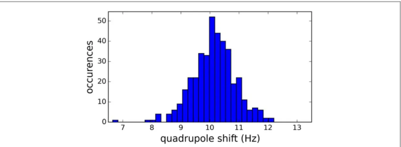
¶ and the resulting quadrupole shift. Infigure4we show the resulting distribution of the QPS. The
distribution shows a mean shift of about 10Hz due to the static axial field gradient of the trap and a standard deviation of 0.74Hz.
In a spherical ion crystal, most of the ions are trapped away from the symmetry axis and the resulting rf-field at the individual ions’ position causes a scalar and TASS. While for Ca40 +the scalar shift can be canceled by
operating the trap at the‘magic’ drive frequency [35], the TASS will result in shifted transition frequencies for
each individual ion depending on its position. We estimate the TASS in our system byfirst calculating the amplitude of the rf-field due to the trap drive at each ion’s position, employing a numerical simulation. The resulting TASS is then estimated by evaluating the time averageá ñ... over one cycle of the squared electricalfield E[27]: f f g J m h E , 4 , 11 J dc 2 d a n = ( ) á ñ ( )
with the dc tensor polarizabilityαdcfrom[74]. Figure5shows the result for our configuration, exhibiting an
approximately uniform distribution with about 25Hz width (see appendixF).
With the distributions as described above, we now turn to the implementation and optimization of the CDD sequence.
For the numerical optimization of the goal function equation(7), we consider a static magnetic field such
that the Zeeman splitting of the S2
1 2states is equal to 10MHz, where the uncertainty of the Zeeman splitting
gsδBis normally distributed with a zero mean and a width of 1kHz. There is also a small contribution due to the
second order Zeeman effect. For the assumed magneticfield noise, this shifts amounts to an additional broadening of about 0.5mHz (averaged over all relevant levels) and can therefore be neglected. In a real experiment, the rf drivingfields used for dressing the states will be imperfect and show some fluctuations. We
Figure 4. Quadrupole shift for the mj= states for 400 ions in a linear Paul trap52 (spherical, isotropic crystal configuration). The
distribution shows a standard deviation of 0.74Hz and a static shift due to trap endcap voltage employed for axial confinement of about 10 Hz.
Figure 5. Tensor shift for 400 ions for the mj
5 2
= states in a linear Paul trap(spherical, isotropic crystal configuration). The shift distribution is calculated for a spherical, isotropic crystal configuration (for details see text). The tensor shift is approximately uniformly distributed with a width of∼25Hz (see appendixF).
estimate the corresponding relative amplitude shifts of the drivingfields δΩto be normally distributed with a
zero mean and a width of 4×10⁻⁴.
In order to test the performance of the scheme in the multi-ion spherical crystal configuration, we have realized the averaged goal function GA, which is given by equation(8), with an average over 100 pairs of {δB,δΩ}
chosen randomly according to the above distributions, and then numerically minimized GAto obtain optimal
driving parameters(all in units of kHz): Ω1=2π×225.3, δ1=2π×95.6, Ω2=2π×13.6, δ2=2π×5,
Ω3=2π×93.6, δ3=2π×27.2, and Ω4=2π×14.8, δ4=2π×25.6. We then integrated the effect of the
counter-rotating terms of the drivingfields and the cross driving fields (the effect of the S2
1 2(2D5 2)drive on
the D2
5 2(2S1 2)states) and adjusted the optimal driving parameters accordingly. We simulated 4927 trials of
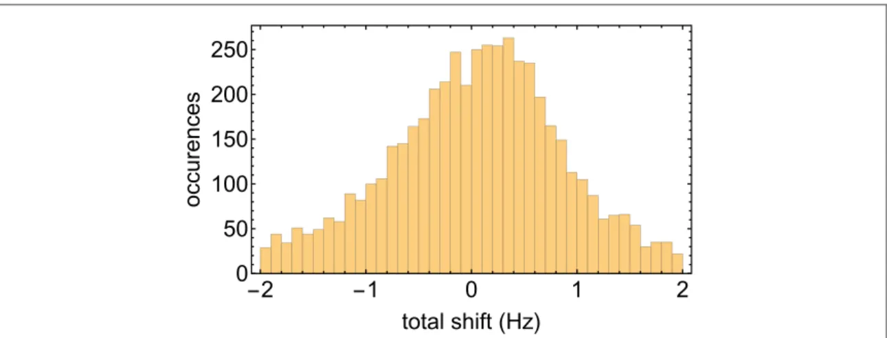
the robust clock-transition with these optimal driving parameters and the above distributions of the Zeeman, quadrupole, tensor and driving amplitude shifts. In the simulations we used the full driving Hamiltonian without making any approximations. For more details see appendicesC–E. The simulation results, shown in figure6, indicate that the shift distribution of the robust transition has a narrow width of∼1Hz.
The distribution shown in thefigure is slightly asymmetric and shifted away from zero. The asymmetry is not a problem when using Ramsey interrogation with short broadbandπ/2 pulses which address all the ions at once, yielding a symmetric(cosine) central resonance. However, the overall shift and the asymmetry lead to a probe-time dependent fractional bias in the clock frequency of around 0.12Hz for a probe time of 150ms, which would have to be evaluated and corrected in absolute frequency measurements.
This shift from the non-perturbed virtual(dressed)2S1 2,mJ = «0 2D5 2,mJ =QJ m, J = transition0 depends on the initial distribution of inhomogeneously shifted line centers and the shift suppression achievable with the selected dynamical decoupling parameters. A qualitative understanding of the influence of different parameters on this shift can be developed from simulation results for the scaling of the shift of the robust transition as a function of the magnitude of the individual shifts, namely, the Zeeman shift uncertainty, quadrupole and tensor shifts, and driving amplitude shift. The simulations shown infigure7were performed with the driving parameters used in the simulations offigure6. For each individual shift, several simulations were conducted with different values of that individual shift while all other shift contributions were set to zero. When varying the magneticfield uncertainty, we see some higher-order (quadratic and cubic) contributions but no linear dependence, showing that the decouplingfields have greatly suppressed the first-order Zeeman shift. This can be understood as an avoided crossing of the dressed levels with respect to the magnetic shift uncertainty δB. The shift of the robust transition as function of the quadrupole and tensor shifts scales linearly. For a perfect
drive of the D2
5 2states(assuming the RWA and no effect of the S2 1 2drive) we expect a quadratic scaling.
However, the S2
1 2drive and the counter-rotating terms of the D2 5 2drive result in an amplitude mixing
between the ideal dressed D2
5 2states, which reintroduces afirst order contribution to the quadrupole and
tensor shifts. The shift of the robust transition as a function of the drive amplitude error scales linearly as the robust transition frequency depends linearly on the drive amplitude. In an experiment the described scaling behavior could be exploited to verify the correct parameter set for the dynamical decoupling scheme by measuring the expected scaling and identifying the correct operating point. Note that the simulations were performed withfixed driving parameters, optimized as described above for a particular distribution of field
Figure 6. Simulation results. Total shift distribution of the robust optical transition in the multi-ion spherical crystal configuration. 4927 simulation trials were realized assuming the following distributions:(i) magnetic field uncertainty—the uncertainty of the S2
1 2
Zeeman splitting is normally distributed with a zero mean and a width of 1kHz, (ii) driving fields uncertainty—the relative drive amplitude uncertainty is normally distributed with a zero mean and a width of 4×10⁻⁴,(iii) quadrupole shift—the quadrupole shift of the mj= states is normally distributed with a mean of −10Hz and a width of 1Hz, and (iv) tensor shift—the tensor shift of the52
shifts and drive amplitudes. For different assumptions on the distribution offield and amplitude fluctuations, different driving parameters could be derived that improve the scheme’s performance case-by-case. Moreover, as in other CDD schemes, the performance of the scheme could, in principle, be improved by adding more drivingfields.
In our analysis we assumed that all drivingfields suffer from driving fluctuations. Generating the second drivingfields (Ω2andΩ4) by a phase modulation, as proposed in [41], should result in stable driving fields with
negligible amplitudefluctuations. In this case we expect a further improvement in the performance of the scheme.
The coupling strength between the dressed S2
1 2states and the dressed D2 5 2states is achieved via the laser
coupling between the bare states that have a non-vanishing amplitude in the desired dressed states. Hence, the effective laser coupling strength is modified by the overlap between the bare states and the single or double dressed states. In our case the laser coupling of the bare2S1 2,mJ = + «12 2D5 2,mJ = + transition is52
reduced by a factor of 0.51(0.3) for the transition between a single (double) dressed S2
1 2state and a single
(double) dressed D2
5 2state. Note that the effective laser coupling strength should in any case be smaller than the
energy gap of the double dressed states, which in our case is∼6 kHz.
Using the results of[25], we estimate the achievable statistical uncertainty of a 400ion Ca+clock when probed with aflicker floor-limited probe laser at 10−14(10−15) to be 5.8´10-16 t s (1.8´10-16 t s).
This represents an order of magnitude improvement in instability over current single ion clocks[3,22,23],
corresponding to a reduction in averaging time by a factor of 100.
5. Applications
One of the many potential applications of the proposed scheme is a cascaded clock[75–77] in which a clock laser
isfirst stabilized to an ensemble of Ca+ions to improve its phase coherence time and thus allow extended probing times[24,25] in a high-accuracy single-ion clock (e.g.Al+or Yb+). To bridge the difference in clock transition frequencies, a transfer scheme using a frequency comb would be employed[77–79]. Table1shows the achievable instabilities of anAl+clock for different initial clock laser instabilities. We have used the results from [25] to determine the optimum probe times assuming flicker-floor limited laser instability and neglecting
spontaneous emission from the excited clock state. Note that after stabilization to the Ca+ion crystal the laser exhibits a white frequency noise spectrum. As expected, the reduction in required averaging time is largest when the initial laser instability is large. As the laser improves, it approaches the quantum projection noise limit of the 400Ca+ions and the gain is reduced. Even higher gain can be obtained from larger crystals or reference atoms
with narrower linewidth than Ca+, such as176Lu+[27,36],88 +Sr [80,81], or138Ba+[82,83]. Our scheme works in
the same way for other atomic species, however, the contribution of the different broadening mechanisms
Figure 7. Scaling of the robust transition shift. The shift of the robust transition as function of(i) the Zeeman shift of the S ;∣ 1 2+ ñ12
state(left), (ii) the quadrupole and tensor shifts of the the D ;2 5 2 ñ52
∣ states(middle), and (iii) the relative amplitude error of the drivingfields.
Table 1. Estimated statistical uncertainties. Theflicker-floor limited performance of the clock laser is denoted by σl,
which is assumed to be independent of the averaging time. The Allan deviations and optimum probe times for different configurations k are denoted by σkand Tk, respectively. The investigated systems are 400Ca+ions using the
described CDD scheme(k=Ca), a singleAl+ion(k=Al), and a cascaded scheme in which a singleAl+ion is probed by a laser pre-stabilized through a cloud of 400Ca+ions(k=CaAl). The reduction in averaging time to achieve a certain statistical measurement uncertainty is given by G.
σl TCa(s) s t( )Ca t s TAl(s) s t( )Al t s TCaAl(s) s t( )CaAl t s G
10−14 0.015 5.8×10⁻¹⁶ 0.003 5 3.6×10⁻¹⁵ 0.25 5.1×10⁻¹⁶ 50 10−15 0.15 1.8×10⁻¹⁶ 0.035 1.1×10⁻¹⁵ 0.78 2.9×10⁻¹⁶ 14
depend on the employed species and specific properties of the experimental setup. We note that in our case a narrower atomic linewidth(as for example provided by a different atomic species such as88 +Sr ) would not necessarily lead to a narrower linewidth of the robust transition, due to the remnant effects of the magnetic noise, the amplitude drive noise and the QPS and TASS. Another reason for using Ca+is the advantageous mass ratio relative toAl+, facilitating efficient sympathetic cooling in anAl+clock[84].
The cascaded clock scheme enables short averaging times with lasers that are commercially available. For state-of-the-art multi-segment ion traps, it is conceivable to trap a large Ca+crystal in one segment and a clock ion in a different segment, strongly reducing experimental overhead. Furthermore, for the case of additional experimental constraints such as a transportable setup or the lack of a cryogenic system, for instance, our scheme could offer an advantage over state-of-the art optical resonators.
Beyond the cascaded clock scheme, many applications in fundamental physics, navigation and industry do not require ultimate accuracy[1,4], but rather high stability as provided by a dynamically-decoupled Coulomb
crystal clock. Through appropriate characterization of the residual line center shift away from an effective
m m
S , J 0 D , J 0
2
1 2 = « 2 5 2 = transition, it is conceivable to not only obtain a reference with small statistical
uncertainty, but also a low systematic uncertainty. In this case, the dynamically-decoupled Coulomb crystal clock would provide a reasonable accurate reference with superior stability.
6. Conclusions
We have proposed a CDD scheme that significantly suppresses the Zeeman shift as well as the quadrupole and tensor ac Stark frequency shifts of an optical clock transition for ion crystals. We analyzed the proposed scheme in the case of a multi-ion crystal of 400 Ca+ions and showed that the shift of the robust transition isd f 1 Hz with a width of∼1Hz, which is close to the observed linewidth when probing the transition for a few hundred milliseconds. Our approach allows to exploit the improved stability from the higher ion number without suffering from the line broadening mechanisms associated with large ion crystals. Our scheme is applicable to other atomic species and experimental setups, paving the way for dynamically-decoupled Coulomb crystal clocks as references with high stability. We would like to note that during the preparation of this manuscript we became aware of a related independent work by Shaniv et al[85].
Acknowledgments
We thank M Barrett for stimulating discussions. We acknowledge support from the DFG through CRC 1128 (geo-Q), project A03 and CRC 1227 (DQ-mat), project B03. This joint research project was financally supported by the State of Lower-Saxony, Hannover, Germany. A R acknowledges the support of ERC grant QRES, project No. 77092.
Appendix A. The dressed states
In this section we present the construction of the(ideal) dressed states. By ideal we mean that there are no noise, uncertainties, or systematic shifts, the RWA is valid, and that the drivingfields of the S2
1 2(2D5 2)do not operate
on the D2
5 2(2S1 2)states.
A.1. The D2
5 2states
The driving Hamiltonian of the D2
5 2states is given by H g BS g g B t S g g B t g t S cos cos 2 cos 2 , A1 D d B z d d B x d d B d x 1 1 2 1 1 2 12 2 m m d m d p d d = + W - + W - + ´ W + -⎡ ⎣⎢ ⎤⎦⎥ ⎡ ⎣ ⎢ ⎢ ⎛ ⎝ ⎜ ⎜ ⎛⎝⎜ ⎞⎠⎟ ⎞ ⎠ ⎟ ⎟ ⎤ ⎦ ⎥ ⎥ [( ) ] ( ) ( )
where gdμBB is the Zeeman splitting due to the static magneticfield B, gd=6/5 is the gyromagnetic ratio of the
D
2
5 2states, Szand Sxare the z and x spin-5/2 matrices, Ω1,Ω2,d =1 18gdW and δ1 2are the Rabi frequencies
and the detunings of the drivingfields, respectively. Moving to the IP with respect to the first drive (Ω1) with
H S g S g g t S 2 2 cos 2 . A2 D I z d x d d y 1 1 2 1 2 12 2 1=d + W + W W +d -d ⎡ ⎣ ⎢ ⎢ ⎛ ⎝ ⎜ ⎜ ⎛⎝⎜ ⎞⎠⎟ ⎞ ⎠ ⎟ ⎟ ⎤ ⎦ ⎥ ⎥ ( )
We continue by moving to the basis of the dressed states with U e S
1= iqd y, where d arccos gd 1 12 21 2 q = d d + W ⎛ ⎝ ⎜ ⎜ ⎞ ⎠ ⎟ ⎟
( )
, which leads to H g S g g t S 2 2 cos 2 , A3 DI 12 d z d d y 1 2 2 1 2 12 2 1= d +⎛ W + W W +d -d ⎝ ⎜ ⎞⎠⎟ ⎡ ⎣ ⎢ ⎢ ⎛ ⎝ ⎜ ⎜ ⎛⎝⎜ ⎞⎠⎟ ⎞ ⎠ ⎟ ⎟ ⎤ ⎦ ⎥ ⎥ ( )and then to the second IP with respect to H02 g2 Sz
2
12 2
d 1 d d
=⎛ W + -⎝
⎜
( )
⎞⎠⎟ . Assuming the RWA,g 2 2 12 2 2 dW1 +d -d W ⎛ ⎝ ⎜
( )
⎞⎠⎟ , we obtain H S g S 4 . A4 D I z d y 2 2 2=d + W ( )The eigenstates ofHDI2are the double-dressed D2
5 2states. The eigenstate with the smallest positive eigenvalue
of1 g 2 2 2 4 2 d 2
d +
( )
W is used for the robust optical transition. A.2. The S21 2states
The driving Hamiltonian of the S2
1 2states is given by H g Bs g g B t s g g B t g t s cos cos 2 cos 2 , A5 S s B z s s B x s s B s x 3 3 4 3 3 2 32 4 m m d m d p d d = + W - + W - + ´ W + -⎡ ⎣⎢ ⎤⎦⎥ ⎡ ⎣ ⎢ ⎢ ⎛ ⎝ ⎜ ⎜ ⎛⎝⎜ ⎞⎠⎟ ⎞ ⎠ ⎟ ⎟ ⎤ ⎦ ⎥ ⎥ [( ) ] ( ) ( )
where gsμBB is the Zeeman splitting due to the static magneticfield B, gs=2 is the gyromagnetic ratio of the
S
2
1 2states, szand sxare the z and x spin-1/2 matrices, Ω3,Ω4,δ3andδ4are the Rabi frequencies and the
detunings of the drivingfields, respectively. Moving to the IP with respect to the first drive (Ω3) with
H01=(gsmBB-d3)szand assuming the RWA g( smBB-d3W3)we get
H s g s g g t s 2 2 cos 2 . A6 S I z s x s s y 3 3 4 3 2 3 2 4 1=d + W + W W +d -d ⎡ ⎣ ⎢ ⎢ ⎛ ⎝ ⎜ ⎜ ⎛⎝⎜ ⎞⎠⎟ ⎞ ⎠ ⎟ ⎟ ⎤ ⎦ ⎥ ⎥ ( )
We continue by moving to the basis of the dressed states with U e s
1= iqs y, where s arccos gs 3 3 2 3 2 2 q = d d + W ⎛ ⎝ ⎜ ⎜ ⎞ ⎠ ⎟ ⎟
( )
, which leads to H g s g g t s 2 2 cos 2 , A7 SI 32 s z s s y 3 2 4 3 2 32 4 1= d +⎛ W + W W +d -d ⎝ ⎜ ⎞⎠⎟ ⎡ ⎣ ⎢ ⎢ ⎛ ⎝ ⎜ ⎜ ⎛⎝⎜ ⎞⎠⎟ ⎞ ⎠ ⎟ ⎟ ⎤ ⎦ ⎥ ⎥ ( )and then to the second IP with respect to H02 32 g2 sz
2 4 s 3 d d =⎛ + W -⎝
⎜
( )
⎞⎠⎟ . Assuming the RWA,g 3 2 2 2 4 4 s 3 d + W -d W ⎛ ⎝ ⎜ ⎞ ⎠ ⎟
( )
, we obtain H s g s 4 . A8 S I z s y 4 4 2=d + W ( )The eigenstates ofHSI2are the double-dressed S2
1 2states. The eigenstate with the positive eigenvalue of
g 1 2 4 2 4 2 s 4
d +
( )
W is used for the robust optical transition.Appendix B. Magnetic and drive shifts
In this section we show how the expansions of the magnetic shifts,ZSiandZDi, the drive shifts,OSiand ODi,
cross-driving effects. In the numerical simulations we took the counter-rotating terms of the drivingfields and the cross-driving effect into account(see appendixC,D). The simulations were performed using the full driving
Hamiltonian without making any approximations(see appendixE). For simplicity we will show the derivation
for the S2
1 2states. The derivation for the D2 5 2follows the same steps.
We start by adding to the driving Hamiltonian of the S2
1 2states, equation(A5), a magnetic noise term,
which is given by gsdBsz. The drive shift is introduced by replacingΩ3andΩ4byW3(1+dW)andW4(1+dW),
whereδΩrepresents a relative shift error of the drivingfields. We assume that the relative errors of the driving fields are correlated since we expect that these errors are mostly due to changes in the amplifier chain and antenna, which are common to all drives. Moving to the IP with respect to thefirst drive as before and assuming the RWA g( smBB-d3W3), we now obtain
H g s s g 1 s g g t s 2 1 2 cos 2 . B1 S I s B z 3 z s x s s y 3 4 3 2 3 2 4 1= d +d + W +dW + W +dW W +d -d ⎡ ⎣ ⎢ ⎢ ⎛ ⎝ ⎜ ⎜ ⎛⎝⎜ ⎞⎠⎟ ⎞ ⎠ ⎟ ⎟ ⎤ ⎦ ⎥ ⎥ ( ) ( ) ( )
We continue by moving to the basis of the dressed states, including the shifts, with U e s
1= iqs y, whereq =s arccos g g 1 s s gs 3 B 3 B2 23 2 d d d d d + + + W + W ⎛ ⎝ ⎜ ⎜ ⎞ ⎠ ⎟ ⎟
(
)
( ) ( ) , which leads to H g g s g g t s 2 1 1 2 cos 2 , B2 SI s s z s s y 3 B 2 3 2 4 3 2 32 4 1= d + d + W +d + W +d W +d -d W W ⎛ ⎝ ⎜ ⎞⎠⎟ ⎡ ⎣ ⎢ ⎢ ⎛ ⎝ ⎜ ⎜ ⎛⎝⎜ ⎞⎠⎟ ⎞ ⎠ ⎟ ⎟ ⎤ ⎦ ⎥ ⎥ ( ) ( ) ( ) ( )and then to the second IP with respect to H02 32 g2 sz
2 4 s 3 d d =⎛ + W -⎝ ⎜ ⎞ ⎠ ⎟
( )
. Assuming the RWA,g 3 2 2 2 4 4 s 3 d + W -d W ⎛ ⎝ ⎜
( )
⎞⎠⎟ , we obtain H g g g s g s 2 1 2 1 4 . B3 SI s s s z s y 4 3 B 2 3 2 32 3 2 4 2= d + d + d + W +d - d + W + W +d W W ⎛ ⎝ ⎜ ⎜ ⎛⎝⎜ ⎞⎠⎟ ⎛⎝⎜ ⎞⎠⎟ ⎞ ⎠ ⎟ ⎟ ( ) ( ) ( ) ( )Assuming now that gs=2, the positive eigenvalue that we consider for the robust clock transition is given by
e 1 4 4 2 1 2 2 8 1 2 4 2 2 1 8 2 2 . B4 s 4 2 32 3 B 2 32 32 4 3 2 32 2 32 3 B 2 3 2 2 4 2 3 2 3 B B2 1 2 d d d d d d d d d d d d d d d d d = + W + + - + W + - + W + W + + + + + W + + W + + + W W W W W [ ( ( ) ( ) ) ( )(( ) ( ) ) ( ( ) ) ( ) ( )] ( )
Following the same calculations for the D2
5 2states and assuming that gd=6/5 we obtain the lowest
positive eigenvalue of the double-dressed D2
5 2states, which is given by
e 1 2 1 100 3 2 2 4 3 16 8 2 10 3 6 9 100 1 . B5 d= ( ( dW2 + dW+ )W +12 dB2+ dBW +1 d2- W1)2+ (dW+ )2W22 ( )
The magnetic shifts,ZSiandZDi, the drive shifts,OSiand ODi, and the correlated shifts, ZOSiand ZODi, are
obtained by the power series expansion of esand edto orders ofd andiB diW.
Appendix C. Modi
fied energy gaps from cross-driving
A drive of the S2
1 2(2D5 2)states also drives the D2 5 2(2S1 2)states off-resonantly and results in a Stark shift of
the initial sub-levels energy gap. For simplicity we will show the derivation for the S2
1 2states. The derivation for
the D2
5 2follows the same steps. Consider the off-resonant drive of the S2 1 2states
Hs ssz gs cos t s , C1 s x 0 0 w w = + W [( - D) ] ( )
wherews0=gsmBBis the Zeeman splitting andΔ is the detuning of the drive. We first move to the IP of the counter-rotating terms of the drive with respect to H s s
z 01= -(w0- D) . This results in H 2 s g s 2 1 2 e e . C2 sI s0 z s x i 2 t i 2 t s s 1= w - D + W⎡ + w0-D s++ - w0-D s -⎣⎢ ⎤⎦⎥ ( ) ( ( ) ( ) ) ( )
We continue by moving to the diagonalized basis of the time-independent part of HsI1with U1=eiqs ys, where
arccos s 2 2 s s gs 0 0 2 2 2 q = w w - D - D + W ⎛ ⎝ ⎜ ⎜ ⎞ ⎠ ⎟ ⎟
( )
( ) ( )H02=2(ws0- D)sz. The time-independent part ofHsI2is given by H 2 2 g s g s 2 4 1 2 2 , C3 sI s s s z s s s g x 0 0 2 2 0 0 2 2 2 s 2 w w w w » D - + D - + W + W + - D - D + W ⎛ ⎝ ⎜ ⎜ ⎛⎝⎜ ⎞⎠⎟ ⎞ ⎠ ⎟ ⎟ ⎛ ⎝ ⎜ ⎜ ⎜⎜ ⎞ ⎠ ⎟ ⎟ ⎟⎟
( )
( ) ( ) ( ) ( )and hence, the eigenvalues are equal to
2 1 s s g g 0 0 2 2 2 2 8 2 2 2 s s s s gs 0 0 2 2 2 1 2 w w D - + D - + + + w w W W - D - D + W ⎡ ⎣ ⎢ ⎢ ⎢ ⎛ ⎝ ⎜ ⎞⎠⎟ ⎛ ⎝ ⎜ ⎜ ⎞ ⎠ ⎟ ⎟ ⎤ ⎦ ⎥ ⎥ ⎥
( )
( )
( ) ( ) ( ), which gives the modified energy gap. Plugging in the parameters of thefirst D2
5 2drive,(W1andΔ = ω0s− ω1, wherew1=gdmBB-d1
and gs=2, we obtained the modified energy gap of the S2 1 2states, which is given by
E 1 4 1 2 . C4 S s s s 1 12 0 1 0 12 12 2 0 12 12 1 2 w w w w w w w w = + W + + + W + + + + W -⎛ ⎝ ⎜ ⎜ ⎞ ⎠ ⎟ ⎟ ( ) ( ( ) ) ( ) For the D2
5 2states the modified energy gap is given by
E 1 5 9 5 2 25 9 1 2 25 9 10 , C5 D d d d 3 32 0 3 0 32 32 2 0 3 2 32 3 2 w w w w w w w w = - W + + + W + + + + W -⎛ ⎝ ⎜ ⎜ ⎞ ⎠ ⎟ ⎟ ( ) ( ) ( ( ) ) ( )
where herewd0=gdmBBand gd=6/5. Expanding the modified energy gaps in a power series of Ω1andΩ3
results in ES s0 s s 0 12 0 2 12 w » + w w w W - and ED d 0 9 25 d d 0 32 3 2 0 2 w » - w w w W
-( ). Note that the second order correction could also be
calculated by an effective Hamiltonian approach.
Appendix D. Correction of the Bloch
–Siegert shift
In this section we give a detailed derivation of the correction of the Bloch–Siegert shift arising from the counter-rotating terms of the drivingfields. Without the correction, we first consider the dressed states due to the rotating-terms of a drivingfield and then consider the effect of the off-resonance counter-rotating terms on the dressed states. These result in an energy shift of the dressed states and(a time-dependent) amplitude-mixing between the dressed states, which is detrimental to the scheme, because it modifies the shifts of the dressed states considered for the robust transition. To correct this effect, wefirst consider the effect of the counter-rotating terms on the bare states, and thenfix the frequency of the drive accordingly, such that the rotating-terms will drive the modified bare states. Consider, for example, the on-resonance driving Hamiltonian
H t
2 2 cos . D1
d= 1sz 2 w2 sx
W + W
( ) ( )
Instead of moving to the IP of the rotating frame, wefirst move to the IP of the counter-rotating frame with respect to H0= - 21sx W and obtain H 2 z 4 z 4 e . D2 t e t I 1 2 2 2 2i 2 2i 2 w s s s s = W + + W + W w + w + - + ( ) ( )
We continue by moving to the diagonal basis of the time-independent part of HI,
H 1 4 4 z 2 e . D3 t e t I» W +1 w2 2+ W22s + 2 s 2i 2 s2i 2 W w + w + - + ( ) ˜ ( ) ( )
If we choose 2w2= 12 4(W +1 w2)2 + W22the rotating terms are on-resonance with the energy gap of the
modified bare states. The on-resonance condition is given by 1
6 2 16 3 . D4
2 1 12 22
w = ( W + W + W ) ( )
In addition, due to the basis change from the basis of the bare states to the basis of the modified bare states, the Rabi frequency of the drive is slightly modified,W W˜ , where2 2
1 2 1 2 4 16 . D5 2 2 2 1 2 1 2 22 2 2 3 2 12 w w w W = W + + W + W + W » W -W + W ⎛ ⎝ ⎜ ⎜ ⎞ ⎠ ⎟ ⎟ ˜ ( ) ( ) ( ) ( )
BecauseW˜2corresponds to an optimal driving parameter, we must take that into account and set the initial Rabi
Appendix E. Numerical analysis
In this section we provide a more detailed description of the numerical analysis of the scheme in the case of a robust multi-ion crystal clock that is presented in section4of the main text.
E.1. Optimized driving parameters
For the optimization of the goal function(see section3in main text and appendixB)
G Z Z O O ZO ZO , E1 i j i j S D i S D j S D j 1, 1 4, 2 B B i i j j j j
å
d d d d = - + - + -= -= = = W W ∣ ∣ ∣ ∣ ∣ ∣ ( )we assume that the magnetic shift uncertaintyδBis normally distributed with a zero mean and a width of 0.5kHz
(so the width of the S2
1 2Zeeman splitting is 1 kHz),d ~B (0, 0.5) kHz, and that the relative drive shiftδΩis
normally distributed with a zero mean and a width of 4×10⁻⁴,d ~ 0, 4´10 4
W ( -). Given these
distributions ofδBandδΩ, we defined an averaged goal function, GA= áG(dmB,dnW)ñmm==100,1,n=n1=100over 100
realizations ofδBandδΩ, which are chosen randomly according to the above distributions. We then numerically
minimized GAover the driving parameters,Ωkandδk. The numerical minimization resulted in the following
driving parameters(all in units of kHz):W =1 2p´225.3,d1=2p´95.6,W =2 2p´13.6,d2=2p´ ,5 2 93.6
3
p
W = ´ ,d3=2p´27.2, andW =4 2p´14.8,d4=2p´25.6. E.2. Fixing the driving parameters
Whenfixing the driving parameters we must take into account the effect of the S2
1 2( D2 5 2) drive on the D2 5 2
( S2
1 2) states (appendixC), as well as the effect of the counter-rotating terms of a drive (appendixD) simultaneously.
We start by parametrically solving the Bloch–Siegert correction equation,2wi= 12 (wi+w0)2 + W - W2i xi˜ , fori
a general detuned drive, where xiwould correspond to the ratio between an optimal drive detuning and Rabi
frequency, that is xi i i
= Wd . We denote the parametric solution ofωibyωsol. Then, in order tofix the driving
parameters of thefirst driving fields, ω1,Ω1,ω3, andΩ3, we numerically solve the following four equations:
ED , , , , , E2 1 sol 3 3 1 1 1 w =w ( (w W) W d W) ( ) ES , , , , , E3 3 sol 1 1 3 3 3 w =w ( (w W) W d W) ( ) E , D , , , , , E4 1 1w1 w3 3 1 d1 1 W = W˜ ( ( W) W W) ( ) E , S , , , , . E5 3 3 3 1 1 2 3 3 w w d W = W˜ ( ( W) W W) ( )
For the case ofμBB=2p´5 MHz (so gsμBB=2p´10 MHz), this results in ω1=2p´5.904 881 MHz, ω3=
2p´9.980 794 MHz, Ω1=2p´225.3107 kHz, and Ω3=2p´93.6311 kHz. The ideal driving parameters,
without the above corrections are given byω1=2p´5.904 411 MHz, ω3=2p´9.972 789 MHz, Ω1=
2p´225.3035 kHz, and Ω3=2p´93.6306 kHz. For the second driving fields we neglect the cross-driving
effect(modification of the energy gap) and take into account only the Bloch–Siegert corrections. We obtain that ω2=2p´160.5892 kHz, ω4=2p´72.0503 kHz, Ω2=2p´13.6373 kHz, and Ω4=2p´14.8157 kHz.
E.3. Simulations
We simulated the full driving Hamiltonian of the system with
H g Bs g s g t s g t t s g t s g t t s g BS g S g t S g t t S g t S g t t S S Q Q 1 cos 1 cos 2 cos 1 cos 1 cos 2 cos 1 cos 1 cos 2 cos 1 cos 1 cos 2 cos 3 I5 2 5 2 1 , E6 s B z s z s x s x s x s x d B z d z d x d x d x d x z T B 3 3 4 3 4 1 1 2 1 2 B 1 1 2 1 2 3 3 4 3 4 2 m d d w d w p w d w d w p w m d d w d w p w d w d w p w = + + W + + W + + + W + + W + + + + + W + + W + + + W + + W + + + - + + W W W W W W W W ⎜ ⎟ ⎡ ⎣⎢ ⎤⎦⎥ ⎡ ⎣⎢ ⎤⎦⎥ ⎡ ⎣⎢ ⎤⎦⎥ ⎡ ⎣⎢ ⎤⎦⎥ ⎡ ⎣⎢ ⎛ ⎝ ⎞⎠ ⎤ ⎦⎥ ( ) [ ] ( ) ( ) [ ] ( ) [ ] ( ) ( ) [ ] ( ) [ ] ( ) ( ) [ ] ( ) [ ] ( ) ( ) [ ] ( ) ( ) where Q and QTrepresent the quadrupole and tensor shifts respectively. First, we simulated the system with
δB=0, δΩ=0, and Q=QT=0 for a time duration of 0.5 s, where we initialized the system in the equal
superposition of 1 S D
2(∣ 1ñ +∣ 1ñ), where∣S1ñand D∣ 1ñare the double dressed S 2
1 2and D2 5 2states with
the smallest positive eigenvalue, respectively. This gave us a reference for the non-shifted transition frequency,
S D
Hz, and QT ~(-3, 0)Hz. Each simulation resulted in a frequency shiftΔν with respect tonS D- . The
histogram ofΔν is shown in figure6in the main text.
Appendix F. Distributions of QPS and TASS
In this section we give some details for the distribution of QPS and TASS.
In the Paul trap we consider for our scheme, the mean rf electricalfield at the position of each ion increases linearly in dependence of the radial distance from the Paul trap symmetry axis. The TASS depends quadratically on the mean electricalfield amplitude f E r
f
2 2
µ á ñ µ
d
( , see equation(11) in the main text ), so that overall we get a
quadratic scaling with distance from the symmetry axis r. We plot the TASS in dependence on the radial distance from the Paul trap symmetry axis infigureF1, showing the expected quadratic behavior. The resulting distribution is shown infigure5of the main text(see also figure 3 in [27]). Note that while the electric field is linear in the radius, the
frequency shifts, being quadratic in thefield strength, vary slowly near the center of the crystal and more rapidly as one moves away from the line of symmetry. Thus, the width of an annulus corresponding to a given frequency interval decreases with increasing radius, roughly compensating for the increasing radial density of ions and leading to an approximately uniform density in frequency space as shown infigure5in the main text. For the purpose of implementation of the numerical simulation, we approximately describe the data with a uniform distribution.
In the numerical simulation of the CDD we neglect possible correlations between TASS and QPS by modeling our system with random samples from corresponding independent distributions. InfigureF2we plot the QPS versus the TASS for each individual ion of our ion crystal. It is evident that the shifts are only weakly correlated. Furthermore, we note that the continuous decoupling drive renders any such correlations insignificant because the remnant effect of the QPS and TASS is a second order effect, and particulary in our case, this effect is much smaller than the effect of the shifts in the amplitudes of the drive, which are the dominant factor that determined the resulting total shift distribution of the robust optical transition(figure6of the main text).
Figure F1. TASS and QPS versus radial distance, i.e. radial distance from the trap’s symmertry axis. For each individual ion, we plot the corresponding TASS and QPS.