Applications of a plume model to photographically observed convection,

PHOTOGRAPHICALLY OBSERVED COLVECTION by

PATRICIA ANN BUDER

B.S., Saint Louis University

1971

SUB MTTED IN PARTIAL FULFILL~ENT OF THE REQU~IRE~MEiTS FOR THE

DEGREE OF MASTER OF SCIENCE at the MASSACHUSETTS IiSTITUTE OF TECHi.OLOGY Kay, i 973 Signature of Autho . . ..

iDe partment of Meteoroiogy 11 May, 1973

Certified by . . . . . .. ~ . .I .~

Accepted by . . . . * * n " " . " . . " . . t Chairman, Departmental Coiamittee

APPLICATIONS OF A PLU~E MODEL TO PHOTOGcAPHICALLY OBSERVED CONVECTION

by

Patricia Ann Buder

Submitted to the Department of Meteorology on 11 May, .1973 in partial fulfillment of the requirements for the degree of Master of Science.

A steady-state entraining plume model was used to pre-dict cumulus convection, and the results were compared to photogramnmetrically observed clouds. The data utilized in this thesis was recorded _{during operation of Cloud Puff IV,} a field experiment undertaken in 1969 in southern New Mexico over the Organ Mountain range. It was noted that the plume model was sensitive to a number of factors, each of which was investigated. Cloud calculations were fond to vary

substantially according to the choice of cloud base level, initial radius and vertical velocity at cloud base and

location of radiosonde sounding input levels. Little sen--sitivity was shown to the houmaidity profile above the level at which dewooint information ceased to be available. Hea-sured cloud base heights seemed to increase slightly with time on each of the three test days. Variability of bases

at a given time was of the order of one thousand feet or less. Error in photogranmetric measurements was sufficient to produce this variability, but it is etirely reasonable

that such differences exist over mountainous terrain.

Cloud base heights were quite close to th. convective con-densation level of the morning sounding on each day and were below both the lifting and convective condensation

levels of the afternoon soundings, Variability of cloud top heights corresponded closely with model predictions from three sets of initi'.l radii and vertical velocities

for each day's medium and large sized clouds. The model was unable to predict with realistic vertical size

pro-files and vertical velocity propro-files the heights of cloud tops for the smaller clouds that were observed. However, an assumption in the model formulation was that the cloud was steady-state and in the mature stage of development, while the observed small clouds were in an initial stage of development.

Thesis Supervisor: Edward N. Lorenz Title: Professor of Meteorology

1. Introduction 4 2. Survey of similar investigations

5

3. Description of the plume model 9

4. Description of the data 12

5. Results of investigation of model sensitivity 14 Sensitivity to choice of cloud base height .14 Sensitivity to choice of sounding levels 17 Sensitivity to choice of initial radius and

vertical velocity 21

Sensitivity to humidity profile 24 6. Model predictions compared with observed growth 26 Description of photograrmetric technique 26

Comparison of predicted and measured cloud

base heights 29

Comparison of predicted and measured cloud

top heights 31

7. Conclusions and Recommendations 33

List of Tables and Figures 37

Acknowledgments 86

1. Introduction

It was desired to make a study of cumulus cloud de-velopment over mountainous terrain, using a numerical con-vection model to predict development and comparing the computed clouds with observations of the convection that actually occurred.

Cloud Puff IV, a field experiment undertaken in 1969 near the Organ Mountains in southern New Mexico, included photographic data from stereo cameras suitable for photo-grannetric measurements. The data from this project was

chosen for use in this investigation because of the availa-bility of these photographs, frequent radiosonde soundings

and other useful information.

With the radiosonde soundings, the plume model written at MIT by Professor Norman Phillips was used to predict the development of convection and the results compared to the dimensions obtained from the photogrammetric measurements. It was found necessary to investigate the sensitivities of the numerical model to initial data input in order to gauge the validity of any results.

The answers to several questions were sought from the predicted and measured results. The numerical model did not account in any way for topographic variation. The question arose of whether the photographically observed

cloud bases were at the sounding's lifting condensation level, the convective condensation level or somewhere in between and. if this could be attributed to lifting by the

less constant height. Is this true over mountains, or is there a large variance in the height at which bases form? Another consideration was whether the variability of predicted cloud tops was comparable to the variability of the cloud tops in the real atmosphere. Perhaps

atmo-spheric conditions vary substantially from one location to another and the clouds that form vary considerably

al-so. Or will a very slight horizontal variation in atmo-spheric conditions, only a few tenths of a degree in tem-perature and dewpoint, produce quite different clouds? It is considerations such as these that are to be inves-tigated in this thesis.

2. Survey of investigations using numerical convection models Several numerical models of cumulus convection have been formulated, and some of the more well known of these will be discussed. The models generally fall into two

classes.

One approach is to set up the complete hydrodynanic equations in finite difference form and allow a computer to solve them in a series of finite tirae steps, beginning with a prescribed initial condition. This type of model is

called a "field of motion" model.

An early such model was described by Malkus and Witt (1959). In this dry model, two-dimensional motions in

ver-a potentiver-al temperver-ature perturbver-ation wver-as introduced ver-and finite difference forms of equations governing vorticity, temperature and motion fields were solved in a series of time steps. The calculations had to be terminated after

a period corresponding to five to seven minutes due to the growth of numerical errors.

Since that time more complicated geometries, the simu-lation of condensation of water vapor into liquid, the

transport of liquid and water vapor and even the effects of the ice phase have been introduced to "field of motion" models. However, such models have been forced to parameter-ize the non-linear processes governing particle growth, since condensation, coalescence, freezing, crystal growth, etc., are analytically intractable processes.

F.W. Murray (1970) has succeeded in modeling the growth and fallout of liquid precipitation. His model is based on the Boussinesq approximation which permits the

derivation of a vorticity equation locally and from this the stream function is found.

Simoson, Wiggert and others from the Experimental Meteorology Laboratory have used numerical models

opera-tionally to predict effects of seeding. Simpson and

Wiggert (1971) used an existing cumulus model and altered it to simulate the dynamic effects of seeding. Wiggert

stituted for the non-fallout of liquid water treatment. The initial perturbation and the observed cumulus tower diameter and cloud base height were presumed to be related. Also, the lower levels of soundings taken over land were restructured to better emulate ambient conditions when clouds grew over the sea,

Another "field of motion" model is that of Gray and Lopez (1972). It is basically one-dimensional and paramet-ric. The turbulent and microphysical phenomena are ex-pressed in terms of cloud-scale variables, while the dyna-mical and thermodynamical processes are treated in a prog-nostic fashion. In order to avoid the coramon similarity assumption, mixing between cloud and environment is para-meterized in terms of the turbulence intensity of the in-terior and exin-terior of the cloud.

The model of Weinstein (1970) is one-dimensional and time dependent. It considers the processes of horizontal mixing, evaporation, precipitation generation and freezing

as well as the dynamic and thermodynamic processes of cumu-li. A slightly modified version of this model was used operationally in Cloud Puff III, a field experiment con-ducted at White Sands, New Mexico, to determine the pre-dicted height of unseeded cumulus tops, the increment of height which would result from seeding and threshold values

an entity, such as a plume or jet, or a bubble. Miajor simplifications result from this likeness. The number of differential equations is reduced, and semi-empirical laws can be derived from theories or measurements of the entity. This allows complete specification of every parameter in the equations except for properties to be predicted.

The Squires and Turner (1962) model and Scorer's bubble theory are of the "entity" type. The plume model used in this thesis is a modified version of the Squires

and Turner model; its properties are discussed under Descrintion of the olume model.

While the "field of motion" type of model seems to suggest a more thorough formulation with an explicit cloud physics treatment, there are serious limitations to its use, some of which apply also to "entity" models. For

example, the results are quite sensitive to the form of the initial perturbation and to the form of expression of the equations in relation to a finite difference grid. It is not at all clear that the present representations of entrainment are completely correct, The "entity" models avoid some of the pitfalls of other models, but they in-troduce assumptions of their own. Nevertheless, a plume model was _{chosen for use in this thesis and its} sensiti-vities were examined.

cloud development that is based on a steady-state, con-densing plume which entrains environmental air by assuming that the inflow velocity at anyr height is proportional to

the upward velocity of the plume. It is a slight modifi-cation of one described by Squires and Turner (1962) and was formulated by Professor Norman A. Phillips of the Massachusetts Institute of Technology and programmed by

Tony Hollingsworth.

The model uses an entropy procedure to account for heat carried by condensed water; it ignores precipitation and assumes the environment has no condensed water. The shape of the cloud and its other properties follow from the dynamics, and cloud development is size-dependendt.

A top-hat profile in combination with the Morton, Taylor and Turner entrainment hypothesis can be used to

express conservation of mass, momentum, water substance and entropy in the saturated plume.

.4 ) 'I 'qr= A r _ .0 4

72

)rr~~,d

where ( = plume density

A- = w~ater rUxing ratio (vapor + liquid or solid) S= specific entropy

S= plume radius

S= plume vertical velocity

and the subscript e refers to the environment.

4(z, the entrainment factor, was taken as 0.1, as was

indicated by the laboratory work of Morton and Turner. Define

tI

The equations then become

0/0- -

D

9/

The integration of these five equations is done by a Runge-Kutta procedure within each of the successive layers defined by radiosonde data. The expressions on the left side of this system are treated as unknowns, to which values must be assigned at cloud base. Squires and Turner assume that the virtual termerature excess at cloud base is zero, since it seems that thunderstorm updrafts derive most of their energy from the latent heats of

con-densation and freezing rather than from surface heat sources, and once triggered merely release the energy stored in the environment. Essentially, it is assumed that at cloud base the specific entropy of the plume equals that of the en-vironment and the plume mixing ratio equals the environ-mental mixing ratio. Thus, the plume is initiated by an updraft at its base, with assigned values of vertical vslo-city and radius, rather than by excess buoyancy at cloud base.

With the proper initial conditions somewhat realis-tic clouds can be simulated. However, the plume model

contains several serious inadequacies. The specification of the initial conditions is arbitrary and the

evolution-ary process of cloud growth is ignored. Lateral growth, the development of downdrafts and drag frora fallirwg pre-cipitation undoubtedly have a marked effect on cloud

dynamics. The above descibed treatment is restr.l~ted to the case of no geneoral wini shear. In mid-latitude convection strong shear is often present, and the assunmp-tion of a vertical _{plume in a non-turbulent environment}

is not valid. _{When the environment is turbulent to a} degree comparable with the updraft an exchange of mass in both directions would necessitate the introduction of detrainment as well as entrainmrent, It appears that a more realistic arrangement would consist of updrafts and

downdrafts, side by side, tilted in the vertical and in-cluding a mass flux in both directions.

4. Description of the data

The data used for this study were collected during operation of Cloud Puff IV, a joint Air Force-Navy-Army field experiment in weather modification, and were ob-tained from Air Force Cambridge Research Laboratories, Bedford, Massachusetts. The principal participants were the Earth and Planetary Sciences Division of the Naval Weapons Center, the Cloud Physics Branch of AFCRL and the Atmospheric Physics Division of White Sands Missile Range. Cloud Puff IV was conducted near Las Cruces, New Mexico

at the White Sands Missile Range, over and near the Organ Mountains,

Of the numerous types of data recorded during this project, in this thesis use was made predominantly of radiosonde soundings and ground based stereo photographs.

Figure 1 _{illustrates the location of the equipment in}

re-lation to the mountain range. The data include transcripts of aircraft crew dialogue recorded during operational flihts over the test area. Occasionally these transcripts provided information on cloud base and top heights. Cloud develop-ment was located in relation to topographic features throtgh mosaic strips assembled from U-2 photographs which were taken from a height of approximately 66,000 feet MSL.

Radiosonde soundings were made at frequent intervals and those used herein were released from White Sands. Data

points were at

500

foot intervals from the surface to

ap-proximately 70,000 feet MSL and higher.

During the three days of operation cited in this study,

15

July 69, 22 July 69 and 25 July 69, vertical wind shear

was observed at all sounding times. On the 15th surface winds were southerly with upper level winds generally from the southeast. Hence, the sounding was upwind of the moun-tains, with convection developing over the range and moving generally westward. The other two days exhibited north-westerly surface winds and considerable vertical shear; in these cases it is observed that the soundings were not up-wind of the peaks.

Morniing and afternoon soundings were used in the plume

model for each of the three test days. The six soundings

tested are shown in Figures 2 through

4.

On 1

5

July 69 and 25 July 69 the 0500 Mountain Standard Time and the

were from 0700 MST and 1300 MST.

Cloud base and top measuArements were made using photo-graphs from the ground based T-11 stereo cameras located near Las Cruces. These cameras wore operated during the period each day from the beginning of cloud formation until

one hour following ternination of the project's final test case, photographs being taken every few minutes. The lo-cation of cloud elements in the vertical was accomnlished through photogrammetric techniques in a manner similar to that described by Glass and Carlson (1963). The photogram-metric methods employed in this thesis are subsequently discussed in detail.

$. Results of investigation of model sensitivity

One of the problems encountered with the plume model is its sensitivity to the input data, e.g., cloud base height, radius and vertical velocity at cloud base, choice

of sounding levels, etc. In order to predict cloud develop-ment with such a model, it was deemed necessary to

investi-gate the effects of such initial specifications on the model's prediction capabilities. Each class of input data was varied over a considerable range. The results were

analy-zed in an attempt to find physically reasonable limits on the choice of each parameter that must be initially specified.

Sensitivity to choice of cloud base height

Since the clouds formed over mountains it as unclear what level would be an appropriate choice for cloud base.

Two different mothods were employed to select a base

height from radiosonde soundings, For a range of initial radii and vertical velocities several runs of the model were made using as cloud base both the lifting condensa-tion level and the convsctive condensation level. Figures

5

through 10 are samples of the graphs used to compile

Table 1. These vertical profiles illustrate the differences in cloud growth. In all cases except one the use of the LCL as cloud base level allowed clouds to become more fully developed, in vertical extent and updraft velocity, than the use of the CCL. This was considerably more pronounced for morning soundings, which had 100 mb to 150 mb

differ-ences between the LCL and the CCL, than for the afternoon soundings, where there were only 10 mb to 20 mb differences. This is reasonable, as more moisture is contained in a

vertical column originatiing at low levels than in one with cloud base at a higher level; in addition, a smaller dew-point depression generally exists at lower levels than at higher levels. Since the growth of the plume is dependent

for the most part on the latent heats of condensation and freezing, the more moisture available, the greater the

de-velopment of the cloud, given a relatively unstable sound-ing.

Four combinations of initial radii and vertical velo-cities, 1000 meters and 1 _{meter per second, 2000 m and 1 mps,} 1000 m and 2 mps, and 2000 m and 2 mps, were used to test the differences in growth between clouds with a base at the

LCL and those with bases at the CCL. Table 1 lists these differences for the sJ~ soundings investigated. For

15 July 69 at 0500 MST the differences ranged from 7100 feet to 11,800 feet. The 0500 MST sounding shows consi-derable low level moisture to be gained by using the LCL of 825 mb rather than the CCL of 664 mb. The 1300 MST sounding of the same day had an LCL of 666 mb, only 10 mb lower than its CCL of 656 mb. The differences in cloud tops were 700 feet to 2t00 feet, considerably less than when the LCL and CCL are more widely separated in height.

These figures accentuate the dependency of cloud growth on the base level chosen; a difference of only 10 mb in cloud base can result in cloud top differences of thou-sands of feet. However, it is not at all clear that this is a product of the plume model and is not the case in the real atmosphere.

The morning sounding for 22 July 69 showed an LCL of 850 mb and a CCL of 760 mb, with cloud top differences ranging from 1500 feet to 5200 feet. Large differences were again encountered with the 0500 MST sounding on 25 July 69, with an LCL of 783 mb and a CCL of 688 mb. The range was 3400 feet to 19,800 feet. These differences

lend support to the idea that the model is quite sensitive to the level chosen as cloud base.

The anomalous case, 1300 IST on 22 July 69, exhibited higher tops using the CCL as cloud base than using the

and the CCL was 654 rmb. Fiigure 11 illustrates the sounding as the comouter interorets it; it is apparent that the com-puter interpretation of the sounding is dependent on the pressure levels that are input. The model ixterpolates between data input levels, and it is seen that the moisture

content of the plume is greatly enhanced in the case of the CCL cloud base as a result of the interpolation procedure. Because of the necessary saturation at cloud base, inter-polation between the initial data point and the next input

level produced greater moisture content in the lowest layer than the model interpreted for the same layer in the case with the LCL as cloud base. Therefore, the higher tops observed in this case are not physically realistic, but rather are a product of a particular choice of sounding

input levels and the computer interpolation procedure.

Sensitivity to choice of sounding levels

As was noted in the previous section, the model pre-dictions are quite sensitive to the pressure levels chosen as data input levels. The model is capable of accommoda-ting up to twenty levels. Initially the assumption was made that significant levels distributed approximately evenly with height would be appropriate, and predictions were made with such data levels. However, the possibility presented itself that the use of more lower levels in place

of the several levels included above 100 mb, while retain-ing highly significant levels, might give a better

repre-sentation of the humidity profile cuhere its fluctuations are most important. With this in mind all previous runs were recalculated using the same initial conditions and

cloud base height, but changing the input levels of the sounding. The results were that in all cases tested cloud growth from a sounding with a more even distribution of input levels with height was greater than from a sounding containing more lower input levels. Figures 12 through 17 illustrate some of the calculated differences. Table 2 gives a complete list of the differences for the cases tested.

To explain this the soundings, as the computer inter-preted them, were plotted on pseudo-adiabatic diagrams and compared. The morning sounding on 15 July 69 is shown in Figure 18. The solid lines are ter4eratures and dewpoints as the computer interprets them given an approximately even distribution of levels with height; the dotted lines are temperatures and dewpoints interpreted from a sounding with more lower levels. Examination of Figure 18 shows that the addition of more lower levels in the sounding reduces the

error from interpolation in the important low layers. The sounding is much dryer than that found from an even distri-bution with height and also contains a more stable layer at upper levels. The combination of these features in this

sounding would tend to cause the model to suppress cloud growth more than in the case where the model is using a sounding with an even distribution.

Again, with the afternoon sounding on 15 July 69, the interpolation of the sounding with levels more evenly dis-tributed with height gives a much more moist sounding than is found when more lower levels are used. See Figure 19. The termerature profiles are much the same except for a shallow stable layer near 1.60 rb for the sounding contain-ing more lower levels. Nevertheless, the moisture differ-ence between the two interpretations of the same sounding is significant enough to cause cloud top differences.

The two interpretations of the 0700 MST radiosonde on 22 July 69 are quite different, as seen in Figure 20.

Again, more moisture is introduced by the interpolation pro-cedure for the even distribution of levels with height in-terpretation, but also the temperature profile is less sta-ble for this case. The introduction of more lower levels to be input allowed a shallow stable layer near 560 mb tc be

detected along with greater stability at upper levels. So once again it is reasonable for greater growth to occur in the case of more available moisture and a less stable tem-perature profile.

The actual differences in cloud tops from the two sounding interpretations, for various initial conditions, are illustrated in Table 2. Cloud top differences were greatest when the base was low, as the LCLs for the mor-ning soundings were; lesser differences were exhibited when cloud bases were high.

envi-ronmental conditions seemed- to be from cloud base to ap-proximately 500 mb. If sounding interpretations differed

in low levels and very high levels and cloud base was chosen above the low level differences, little variation in pre-dicted cloud size occurred. The morning sounding on 15 July 69 with the CCL as cloud base level is a case in point.

For 1300 MST on 15 July 69 using _{the LCL of 666 mb as} cloud base the range in cloud top differences was zero to 4800 feet. But the use of the CCL of 656 mb, only 10 mb higher, as cloud base for the some sounding interpretation

gives a range of 700 feet to 100O feet, considerably less. This is explained by noticing on Figure 19 that the choice of a base at 656 mb reduces the excess moisture produced by the interpolation procedure for the even distribution with height sounding interpretation to third to one-half of the amount present with base at the LCL.

The cloud top differences for the 0700 MST radiosonde on 22 July 69 were 1500 feet to b00 feet with the base at

the 850 mb LCL and 400 feet to 3600 feet with the base at the 760 mb CCL. These values exhibit a less marked differ-ence between the case with the LCL as cloud base and the case with the CCL as cloud base; this is due to more sta-bility and less moisture distributed throughout the

sound-ing with more lower input levels than for the same soundsound-ing with a more even distribution of inout levels. Thus the

choice of a higher cloud base level does not avoid most of

soundings, as was true in the two previous cases.

For the three soundings used in this section, the choice of more lower ixnout levels caused cloud top heights to be consistently lower than did the choice of levels more

evenly distributed with height. The explanation for this was nearly the same in all cases: more moisture than was actually present was introduced by the interpolation pro-cedure when low sounding levels were farther apart. Con-ceivably, the reverse could be true, presumably with the opposite result. In any case, it is evident that for very

small changes in atmospheric conditions in a vertical col-umn the model can produce quite different clouds. However, this may be a property of the real atmosphere as well.

Sensitivity to choice of initial radius and vertical velo-city

Along with other initial specifications, the plume model requires an initial radius and vertical velocity at

cloud base to be inout. In addition to the aforementioned sensitivities, the model was found to be quite sensitive to these initial conditions,

It was decided that a very wide range of combinations of initial radii and vertical velocities would be input to test the modelts capabilities and to determine the proper range on the variables to be used when computing clouds to be compared with measured clouds. The radii used were 100, 500, 1000, 2000, 10,000, and 1,000,000 meters. Vertical

velocities were 0.5, 1, 2, 5, and 10 meters per second. All thirty combinations of theso variables were comouted for the morning sounding of 15 July 69 with both the LCL and the CCL as cloud base and for the afternoon sounding of the same day with the LCL as cloud base. Figures 21 through 29 are examples of the v ertical profiles which result.

In all cases tested the most realistic profiles were obtained with the initial conditions of 500,2; 1000,1; 1000,2; 2000,1 and 2000,2. For certain soundings and bases other combinations gave reasonable profiles, but the above five were consistently acceptable. After an examination of the clouds in the photographs it was de-cided that the four combinations 1000,1; 1000,2; 2000,1 and 2000,2 would be used. Of course, there was a wide range in predicted cloud top heights with all combinations, including the above four.

Very small initial radii and vertical velocities often exhibited vertical profiles with a sharp decrease and then increase of radius with height. The vertical velocity then reached unrealistically high values in low levels, corres-ponding to the point at which the radius became so small.

It is unclear exactly what feature of the model produces this, but it is thought that possibly the treatment of en-trairnment causes such behavior, since a very large propor-tion of such a small cloud would be entraining.

coupled with a relatively smal.l initial radius, the comput-ed plume radius increascomput-ed slightly, decreascomput-ed and then in-creased again. Some simpole calculations made with a simi-lar but dry model suggest this is natural behavior for the plume, given an unstable sounding. In fact, dry calcula-tions suggested this may be natural behavior in all cases, though it does not seem to be the result in most of the other cases tested. It was thought that perhaps the radius

did increase initially, however slightly, in all cases but that it decreased again quite rapidly, before the first

level of print-out was reached. To check this, runs were made with the number of interpolation points between

sound-ing input levels increased, with the values of variables printed out for each interpolation point. There was no

evidence, however, that the radius initially does increase with the wet model, as was suggested by hand calculations with the dry model.

In a few cases, the plume radius at the end of upward motion increased to extremely large values. The vertical velocity was very small in these cases. The large radii would be produced by the requirement that the mass flux be finite. As the vertical velocity approaches zero, the

rad-ius must approach infinity due to the mass flux constraint. A basic assumption made in foriulating the plume

model is that the plume is tall and narrow. Scaling as-sumptions are made accordingly, so the use of a very large radius is inappropriate. Nevertheless, out of curiosity

a synoptic scale radius, orne million meters, was input. Surprisingly, realistic vertical profiles resulted with most initial vertical velocities. Regardless of the ini-tial vertical velocity, the clouds with the large iniini-tial radius all grew to the same height. Figures 30, 31 and 32 illustrate the three test cases, A possible explanation of this is as follows. A cloud with a large radius is affect-ed very little by entrainment. A great deal of energy is contained in such a cloud, derived predominantly from the latent heats of condensation and freezing. The initial impulse created by a specified vertical velocity- _{at cloud}

base is a very small proportion of the total energy of the cloud, and cloud growth would therefore be governed by la-tent heat release, which is the same for a given sounding and cloud base height. Thus, all clouds with the large initial radius would reach the same height.

Ten thousand meters was also input as an initial rad-ius. Figure 33 is an example of the computed profiles. Cloud growth was similar to that for one million meters, but with a slight variation in cloud tops with input

ver-tical velocity. A similar explanation would apply to this case.

Sensitivity to humidity profile

It is well known that the devwoint sensor in radio-sonde equipment ceases to give representative values at high levels. Since some of the sounding input levels

were always above the :level at Jwhich dewpoints no longer were available, the question arose of what value to input

in lieu of a reading. The plum-e model is programmed to receive texrperature al;d dewpoiat data in the same coded form as it is relayed on National Weather Service teletype circuits, that is, a coded fivs digit group with tempera-ture and dewpoint depression. It was thought that the layers for which dewpoint measurements were not available contained only a small percentage of the total moisture in the plume, so the sounding was dryed out in these layers by inserting a 99 for dewpoint depression in the code grouo. However, to be certain the effect of the moisture in these upper layers was minimal a check seemed advisable. Runs were made for comparison that were identical to the dried out runs except that a constant reltative humidity, equal to that at the last known level, was maintained for the re-mainder of the sounding.

The results showed no change in any variable through-out the vertical extent of the plume except for the radius at the end of upward motion, in a few cases. The vapor, liquid and solid water contents were the same whether the humidity was constant or the sounding was dried out above the last known dewpoint data point. The differences in radii were negligible, ranging fr'cm zero to only 7- - meters. Possibly this was a result of the integration technique. In any case, the pluoe does not seem at all sensitive to humidity variations in the ure. levels.

6. Model oredictions com ared ivtwth observed growth

Having investigated the limitations of the plume model, it remains to predict cloud development with it and -com)are the results to what actually formed in the atmosphere.

Photogrammetric techniques were employed to obtain measure-ments of real clouds, but some problems were encountered in implementing the techniques. Variability was encoun-tered in many aspects of this study, e.g., in the plume model calculations, in photogrammetric measurements, in the real atmosphere. The question is whether the amount of variability displayed is physically realistic and com-parable to that of the real atmosphere.

Description of ohotogramnmetric techniques

The heights of cloud bases and tops were desired for the three test days; they were obtained from simultaneous stereo photographs taken every few minutes. The cameras were located at the ends of a baseline oriented perpen-dicular to the azimuth 151.28* from true north. The dis-tance between cameras was 7894 feet, and the cameras were mounted so that the focal plane was perpendicular to the horizontal.

The photogrammetric procedure is based on the prin-ciple of parallax measurement. The range Y of a point in space is determined from the following equations for the normal case of photogrammetry. These equations assume the

oriented horizontally.

I,

B

where

.x

is _{the baseline distance perpendicular to the} camera axis, f is the focal length (assumed the same for both cameras) and P is the parallax, Figure 34. illus-trates the geometry for parallax in the normal case.

where (' and X' are shown in Figure _{31L. ' is obtained} in a similar manner. The values x' and 4' are found with respect to fiducial lines on the reference photograph,

which in the case illustrated is that photograph taken with the north camera. The coordinates

X

and

Z

are positive eastward and upward, respectively.

The above equations were used for measurements on 22 July 69 and 25 July 69. Calculations made of distances and heights of peaks with known values and known azimuths showed the optical axes of the cameras to be very nearly parallel on these days.

Triangulations done from the 15 July 69 photographs revealed the optical axis of the norith camera to be oriented 1.2 to the right of the perpendicular to the baseline.

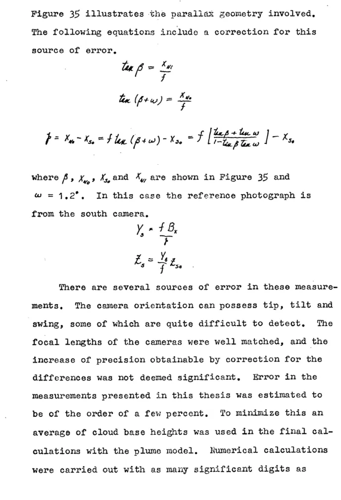
Figure 35 illustrates the parallat geometry involved, The following equations include a correction for this source of error.

where".. X4,

,-where , Xo, J4 and X, are shown in Figure 35 and

= 1,2. In this case the reference photograph is

from the south camera.

There are several sources of error in these measure-ments. The camera orientation can possess tip, tilt and

swing, some of which are quite difficult to detect. The focal lengths of the cameras were well matched, and the increase of precision obtainable by correction for the differences was not deemed significant. Error in the measurements presented in this thesis was estimated to be of the order of a few percent. To minimize this an

average of cloud base heights was used in the final cal-culations with the plume model. Rumerical calcal-culations were carried out with as many significant digits as

measurements allowed,

Comarison of predicted and _{measured cloud base heights} Using photogramnnetric technioues the heights of cloud bases and tops were measured from photographs taken on the three test days. Table 3 lists the results of these mea-surements.

The measured base heights increased slightly with time on each day. Figure 36 is a plot of cloud base height with time. Considerable scatter exists, but uhat curve fitting was possible seemed to indicate an increase in cloud base height with time on all three days. This was probably a result of heating over the mountains which would slightly modify atmospheric conditions in the vicinity of the cloud. Clouds that formed previously in a particular area would also contribute to a redistribution of heat and moisture and an alteration in the level at which the formation of new clouds would occur,

The heights of cloud bases on a particular day were found to vary by as much as 2000 feet, but generally varied by approximately 1000 feet. At any given time the variation was one thousand feet or less. Over the plains it has been

noted that cloud bases generally form at nearly the same level. Although the measurements in this investigation

suggest that this is not true over the mountains, the varia-tion could easily be attributed to error incurred by the crudity of the photogra~metric techniques employed here. However, it seems entirely _{possible and even probable that}

there would indeed be varition in cloud base heights over mountains. The forced .rechanical lifting of the terrain and particularly an elevated heat source with substantial horizontal variation would undoubtedly produce horizontal variation in atmospheric conditions sufficient to cause cloud formation at different heights. Nevertheless,. since it is not known whether the discrepancies encountered were real or a result of error in measurements, an average of measured cloud bases was taken and is listed in Table 3.

It is seen that the average base for 15 July 69 was

705 mab. However, one of the cloud base measurements for that day was considerably lower than all other measured bases, as the cloud considered was over the plains west of the mountains, It was decided that thi measurement was not representative of bases over mountains, and it was not included in a new base average calculation. The average base for this date was recalculated to be 679 mb, which is

slightly below the morning CCL of 664 mb, but well above the LCL of 825 mb. The average base was below both the 666 mb LCL and the 656 mb CCL of the afternoon sounding.

On 22 July 69 the average measured base was 733 mb, which was above the 850 mb LCL and the 760 mb CCL of the morning sounding. The average base was below both the

LCL of 680 mb and the CCL of 651, rib of the afternoon sounding.

For 25 July 69 the average base was only 1 mb higher than the morning CCL of 688 rmb, It was higher than the

morning LCL of 783 mb aid lowev - t an the afternoon LCL/COL of 653 mb.

It is seen that in.all cases the average measured bases were quite near the CCL of the morning scanding and lower than the LCL or CCL of the afternoon sounding. This sug-gests that the primary factor contributing to the convec-tion being studied is surface heating, although the simple process by which the CCL is obtained may not be entirely appropriate over mountainous terrain. Nevertheless, pre-vious studies over similar isolated peaks have suggested that heating is the primary process contributing to con-vective development and that lifting is minimal due to

air flow around rather than over the peaks.

Comparison of nredicted and measured cloud top heights

The heights of the measured cloud tops varied substan-tially for each day. For comparison clouds were computed for each day from the morning and afternoon soundings, using the average measured cloud bases and four sets of

initial conditions. The vertical profiles for each case are shown in Figures 37 through 42. The results appear in Table 14. An examination of this table reveals that ini-tial radius 2000 m and vertical velocity 2 mps consistently over-predicted cloud top heights. Therefore, consideration was made of the remaining predictions, excluding those made with 2000 m and 2 raps. The justification for this is that the choice of initial conditions is somewhat arbitrary

anyway, and the values of 2000 m and 2 mps may be too large. Looking only at clouds that formed over the mountains, measured tops ranged from 14,100 feet to 23,700 feet on 15 July 69. From the morning sounding computed cloud tops ranged from 21,800 feet to 30,000 feet; the afternoon sound-ing gave a range from 19,1100 feet to 25,300 feet.

For 22 July 69 measured tops were 11,900 feet to

34,100 feet. Computed tops were 24,400 feet to 36,200 feet from the morning radiosonde and 22,200 feet to 35,600 feet from the afternoon sounding.

From the 25 July 69 photographs, cloud tops were found to vary from 13,-00 feet to 22,400 feet. Computed tops from the morning sounding were 19,700 feet to 21,000 feet and 19,300 feet to 22,300 feet with the afternoon

sounding.

Some of the small clouds measured are not duplicated by computation. It is known and has been previously

dis-cussed that unrealistic profiles are obtained with small initial conditions. However, the measured small clouds were obviously in the initial stage of development, while

the plume model assumes the cloud is steady-state and in the mature stage of development. Therefore, this model could not be expected to predict the heights of such in-fant clouds.

In the range of medium and large clouds relative to a particular day, the model predicts quite well with both the morning and afternoon soundings. In general,

cloud tops produced by, the real atmolsphere correspond close-ly to those produced by the plune imodel. For example, on 22 July 69 the larger clouds' tops were predorminantly in the 25,000 to 35,000 foot range. The model produced cloud tops in this range quite faithfully. An even rmore striking example is the case of 25 July 69. The larger clouds

ranged from 17,000 feet to 22,000 feet. Predicted clouds ranged from 19,000 feet to 22,000 feet.

Conclusions and Recommendations

It has been shown that the entraining convective plume model used in this research is quite sensitive to a variety of factors, and that the choice of these factors has a di-rect effect on the outcome of a comparison of model clouds with observed clouds.

Using an identical sounding and initial radius and vertical velocity the plume model produces cloud tops that

differ by thousands of feet when different cloud base levels are chosen. A difference of only 10 rb in cloud base can result in largely different cloud tops.

Cloud growth is also highly dependent on the choice of sounding levels to be input. In the cases tested the use of more lower levels, to gain a better representation of the low level humidity profile, produced consistently smaller clouds than did a sounding with a more even dis-tribution of levels with height, all other input para-meters being equal. An exasination of the two computer

interpretations of the sounding revealed that the

inter-polation procedure caused i;iore moisture to be present in low levels when an even distribution was input. Although this particular result was found in all cases tested, the opposite could easily occur.

The plume model was tested with a wide range of initial radii and vertical velocities at cloud base. For very small initial conditions unrealistic vertical profiles and verti-cal velocities were produced. Very large initial radii, although violating the scaling assumptions made in forrau-lating the plume equations, nevertheless gave somewhat realistic profiles. However, the initial radii and velo-cities of 1000,1; 2000,1; 1000,2 and 2000,2 were judged most applicable to the convection being studied.

A test of the model's sensitivity to the hiumidity input above the level where dewpoint information was no longer available showed virtually no change in the output, whether the sounding was dried out or maintained at a

constant relative humidity. Evidently the amount of mois-ture above that level is so small a percentage of the total moisture that cloud development is independent of it.

Measured cloud bases were found to increase with

time on all three days, probably a result of surface heat-ing. The variability of cloud base heights at any given time on a particular day was one thousand feet or less. Error in photogranmetric measurements was sufficient to account for this, but it is also reasonable to assume that

variation in cloud base height does exist over mountainous terrain, as horizontal variation in surface heating is pre-sent. _{Actual cloud bases were found to be quite near the} convective condensation level of the morning sounding. Bases in all cases were below both the LCL and the CCL of the afternoon soundings. These findings suggest that an elevated heat source is dominant in determining cloud base height and the effect of lifting is minimal. Other studies

over isolated peaks have obtained similar results.

Cloud top heights were predicted using the four sets of initial conditions previously mentioned and the average measured cloud base heights. Initial radius 2000 m and

vertical velocity 2 mps were found to over-predict. The remaining predictions corresponded closely with measured heights for the mediuri and large clouds observed on each

day. The model did not predict cloud top heights for

smaller clouds, as they were not observed to be in a mature stage of development.

For more conclusive results it is recommended that more than one type of convection model be used for purposes of prediction. Perhaps a "field of motion" model and an

"entity" model should both be used and their results com-pared as well as a comparison with observed clouds. Of course the sensitivities of any model used for such pur-poses must be thoroughly explored.

The photograrfmetric techniques are subject to con-siderable error and mwny measurements should be made to

obtain a large sample. More sophisbicated techniques

should be employed than were possible for this thesis, such as a computer program that corrects for camera tip, tilt and swing, as discussed by Glass and Carlson (1963).

The use of the above models and techniques could pre-sumably serve to further clarify the nature of convection.

List of Tables and Figures Table

1. Cloud top differences between LGL cloud base and CCL cloud base

2. Cloud top differences between sounding with even dis-tribution with height and one with more lower levels

3. Photogrammetrically measured cloud bases and tops

4.

Comparison of measured cloud tops and computed cloud

tops

Figure

1. Map of Organ ountains and vicinity

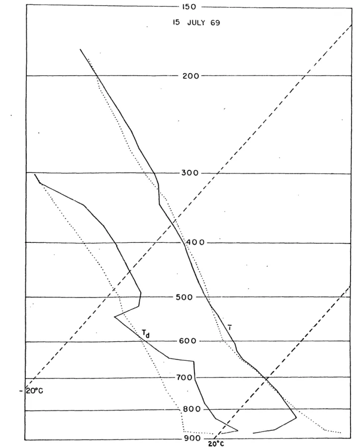
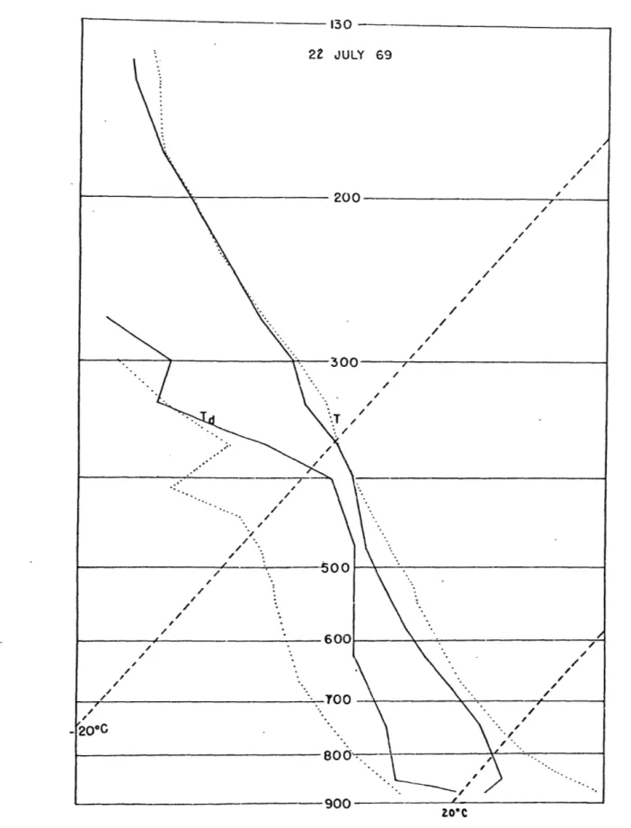
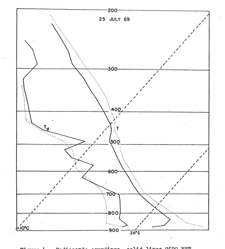
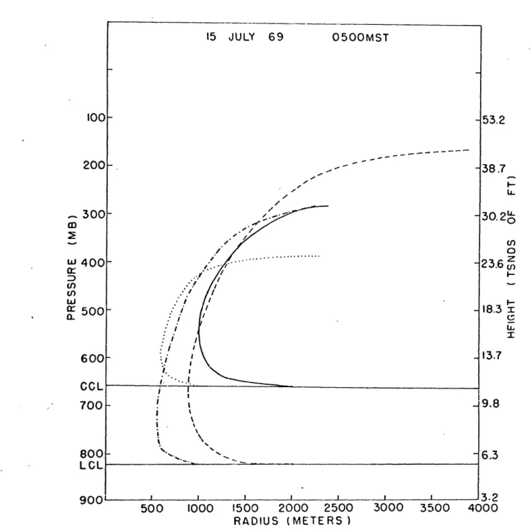
2. Radiosonde soundings, 15 July 69, 0500 MST and 1300 MST 3. Radiosonde soundings, 22 July 69, 0700 EMST and 1300 MST 4. Radiosonde soundings, 25 July 69, 0500 MST and 1300 IST 5. Plume profiles with bases at

0500 MST, initial conditions 6. Plume profiles with bases at 0500 XST, initial conditions 7. Plue profiles with bases at

1300 MST, initial conditions 8. Plume profiles with bases at

1300 MST, initial conditions 9. Plume orofiles with bases at 1300 MST, initial conditions 10. Plume profiles with bases at

1300 MST, initial conditions

LCL and CCL for 15 July 69

1000,1 and 2000,1

LCL and CCL for 15 July 69 1000,2 and 2000,2

LCL and COL for 15 July 69 1000,1 and 2000,1

LCL and CCL for 15 July 69 1000,2 and 2000,2

LCL and CCL for 22 July 69 1000,1 and 2000,1

LCL and CCL for 22 July 69 1000,2 and 2000,2

11. Computer interpretation of radiosonde sounding, 22 July 69, 1300 MST

12. Plume profiles from two compouter interpretations of 15 July 69, 0500 XST sounading, base WL, initial condi-tions 1000,1 and 2000,2

13. Plume profiles from two coliputer inte.retations of 15 July 69, 0500 IST sounding, base LCL, initial

condi-tions 2000,1 and 1000,2

14. Plume profiles from two corrouter interpretations of 15 July 69, 1300 IST sounding, base CCL, initial condi-tions 1000,1 and 2000,2

15. Plume profiles from two computer interpretations of 15 July 69, 1300 MiST sounding, base CCL, initial condi-tions 2000,1 and 1000,2

16. Plume profiles from two computer interpretations of 22 July 69, 0700 MST sounding, base LCL, initial condi-tions 1000,1 and 2000,2

17. Plume profiles from two computer interpretations of 22 July 69, 0700 MST sounding, base LCL, initial

condi-tions 2000,1 and 1000,2

18. Two computer interpretations of 15 July 69, 0500 MST radiosonde sounding

19. Two comouter interpretations of 15 July 69, 1300 MST radiosonde sounding

20. Two computer interpretations of 22 July 69, 0700 I'ST radiosonde sounding

21. Plume profiles, 15 July 69, 0500 MST, base LCL, ini-tial conditions 100oo,o0.5; 00o,0.5; 1000,0.5; 2000,0.5 22. Plume profiles, 15 July 69, 0500 MST, base LCL,

ini-tial conditions 100,5; 500,5 and 1000,5

23. Plume profiles, 15 July 69, 0500 lIST, base LCL, ini-tial conditions 100,10; 500,10 and 1000,10

24. Plume profiles, 15 July 69, 0500 MST, base CCL, ini-tial conditions 100,10; 500,10; 1000,10 and 2000,5 25. Plume profiles, 15 July 69, 1300 MST, base LCL,

ini-tial conditions 100,0.5; 500,0.5; 1000,0.5; 2000,0.5 26. Plume profiles, 15 July 69, 1300 MST, base LCL,

ini-tial conditions 100,1; 500,1; 1000,1 and 2000,1

27. Plume profiles, 15 July 69, 1300 MST, base LCL, ini-tial conditions 100,2; 500,2; 1000,2 and 100,5

28. Plume profiles, 15 July 69, 1300 MST, base LOCL, ini-tial conditions 500,5; 100,10 and 500,10

29. Plume profiles, 15 July 69, 1300 MST, base LCL, ini-tial conditions 2000,2; 1000,5; 2000,5 and 1000,10

30. Plume profiles, 15 July 69, 0500 IMST, base LCL, ini-tial conditions 1,000,000 radius and 0.5, 1, 2, 5, 10 vertical velocity

31. Plume profiles, 15 July 69, 0500 MST, base CCL, ini-tial conditions 1,000,000 radius and 0.5, 1, 2,

5,

10 vertical velocity

32. Plume profiles, 15 July 69, 1300 MST, base LCL, ini-tial conditions 1,000,000 radius and 0.5, 1, 2, 5, 10 vertical velocity

33. Plume profiles, 15 July 69, 1300 MST, base LCL, ini-tial conditions 10,000 radius and 0.5, 1, 2,

5,

10 vertical velocity

31. Parallax geometry for normal case

35. Parallax geometry, north camera 1.2' to right of per-pendicular to baseline

36. Cloud base height versus time from photogrammetry 37. Plume profiles, 15 July 69, 0500 MST, base 679 nib,

initial conditions 1000,1; 2000,1; 1000,2 and 2000,2 38. Plume profiles, 15 July 69, 1300 MST, base 679 mab,

initial conditions 1000,1; 2000,1; 1000,2 and 2000,2 39. Plume profiles, 22 July 69, 0700 MST, base 733 mb,

initial conditions 1000,1; 2000,1; 1000,2 and 2000,2

40.

Plume profiles, 22 July 69, 1300 MST, base 733 mb,

initial conditions 1000,1; 2000,1; 1000,2 and 2000,2 41. Plume profiles, 25 July 69, 0500 EiST, base 687 mb,

initial conditions 1000,1; 2000,1; 1000,2 and 2000,2 42. Plume profiles, 25 July 69, 1300 IMST, base 687 mb,

Table 1

Cloud top differences between LCL cloud base and CCL cloud base

time LCL and radius (m)

CCOL & vert. vel. (mps)

0500

LCL-825

CCL-66L 1300 LCL-666 CCL-656

0700

LCL-850

CCL-760

1300

LCL-680

CCL-654

0500 LCL-783

CCL-688

1300

LCL=CCL

653

1000,1 2000,1 1000,2 2000,2 1000,1 2000,1 1000,2 2000,2 1000,1 2000,1 1000,2 2000,2 1000,1 2000,1 1000,2 2000,2 1000,1 2000,1 1000,2 2000,2 cloud top differences (feet)

7500

9000

7100

11800

700

1900

700

2400

1500

3800

3500

5200

-2500 - 500

-1300

-3500

3400

17700

5900

19800

none date

7-15-69

7-15-69

7-22-69 7-22-69

7-25-69

7-25-69

Table 2

Cloud top differences between sounding with even distri-bution with height and one with more lower levels

radius (m)-& vert. vel.

(mps) 1000,1 2003,1 1000,2 2000,2 1000,1 2000,1 1000,2 2000,2 1000,1 2000,1 1000,2 2000,2 1000,1 2000,1 1000,2 2000,2 1000,1 2000,1 1000,2 2000,2 1000,1 2000,1 1000,2 2000,2 cloud top difference (feet) 1400 0 2200 3300

300

0 0 0 0 800 1700

4.800

600

1400

700 1100

54oo

1700

1500

3300 400 3600 2000 3100 date time 7-15-69

7-15-69

7-15-69 7-15-69 7-22-69 7-22-69 base

LCL-825

CCL-664 LCL-666

CCL-656

LCL-850

00CCL-760 0500

0500

1300 1300 0700 0700

Table 3

Photogrammetrically meas.ured cloud bases and tops time cloud base (ft) cloud base (mb) cloud top (ft) 14:33 16:05 16:30

6375

11 ,790 11 , 257

9935

12,118 16:00 8436 9108 16:15 8965 9291 16:33 9402 9028 17:20 9324 10.020 14:23 14:35

14:49

10,343 10,782 11,035 11,365

'11,396

date _range (ft) 7-15-69 7-22-69

7-25-69

810 666 681 712

658

753

735

739

730 728

737

730 712 703 692

685

677 676 10,661 23,691

15,461

14,139 1 6,322 33,429 32,137 16,291

34,064

11-901 26,623 15,168

15;,500

17, 945 20,175 22,1.435 13,525

13,533

53,000 103,000 97,000 89,000 100,000 98,000 130,000 147,000 103,000 115,000 90,000 128,000

81,00ooo

86,000 110,000 112,000

49,000

105,000

Table

4

Comparison of measured cloud tops and computed cloud tops

date

7-15-69

time measured tops (ft) 14:33 16:05 16:30 7-22-69 16:00 16:15 16:33 17:20 7-25-69 14:23 14:35

14:49

10,661 23,671 15,461 1l,1 39 16,322 33,429 32,137 16,291

34,06

11,901 26,623 15,168

15,500

17,9145

20,175

22,435 13,525 13,533 radius (m) & vert. 1000,1 2000, 1 1000,2 2000,2 1000,1 2000,1 1000,2 2000,2 1000,1 2000,1 1000,2 2000,2 vel. morn. soundi 21 ,800 30,000 25,100 33,900 24,400 36,200 29,500 40,100 19,700 21 ,000 20,800 25,000 computed tops (ft) aft. ng sounding 1 9,400

25,300

21,300 33,800 22,200 35,600 26,400 43,100 19,300 22,300 21,500 24,200

4 5F 30 7Stero pelf 10 20 170 100.000. so 300!00 10O 2 3 4 5 6 7 S 20 4 0 1 i t 4 6 ; r 9 40 I.

I Iiii ii Ii ~j.I.I.JJLII~1.1~tL.L~JJ~~iLIIi.~l~iII.I~J IilitIIII i lii ltilii itiit ili i~~t littit ili I II iiiiliitlti ii 111111

Figure 2. Radiosonde soundings, solid lines 0500 MST, dotted lines 1300 MST.

ZO'C

Figure 3. Radiosonde soundings, solid lines 0700 MST, dotted 1 300 MST,

Figure 4. Radiosonde soundings, solid lines 0500 IMST, dotted lines 1300 MST.

15 JULY 69 0500MST io00- _- 53.2 200 _

38.7

m 300 _{-30.2 u.} O w 400 - 23.6 i c

/I-w

1,- I-a. 500 -8. 600- - 13.7 CCL 700 i I - 9.8 800. -6.3 LCL .- .... -900 I I I I 3.2 500 1000 1500 2000 2500 3000 3500 4000 RADIUS (METERS )

Figure 5. Plume profiles with bases at LCL and CCL, dotted line and dot-dash line irnitial conditions 1000,1; solid line and dashed line initial conditions 2000,1.

15 JULY 69 0500MST 100 -53.2 200 -. _-38.7 -300- _{- 30.2} //(f) / 0 U 400 , - 23.6 or" .," F-S 500 / - 18.3 I 600 i 13.7 CCL 700- -9.8 800- -6.3 LCL 900 _ __ _ i i 3.2 500 1000 1500 2000 2500 3000 3500 4000 RADIUS (METERS)

Figure 6. Plume profiles with bases at LCL and CCL, dotted line and dot-dash line initial conditions 1000,2; solid line and dashed line initial conditions 2000,2.

I-L_ 300- _{30.2 L} 2 o 400- 23.6 z 500 -18.3 -LCL 700- - 9.8 800 - 6.3 900 3.2 500 1000 1500 2000 2500 '3000 3500 4000 RADIUS ( METERS )

Figure 7. Plume profiles with bases at LCL and CCL, dotted line and dot-dash line initial conditions 1000,1; solid line and dashed line initial conditions 2000,1.

r 400 - - 23.6 z (.1) / -S500 " -18.3 . I I 600 .. 13.7 CCL LCL 700 - 9.8 800 - 6.3 900 I 3.2 500 1000 1500 2000 2500 3000 3500 4000 RADIUS (METERS )

Figure 8. Plume profiles with bases at LOCL and CCL, dotted line and dot-dash line initial conditions 1000,2;

I-Cr 4 0 0 23.6 u_ cn a. 500 18.3 z 60-600 "" _{13.7 I} CCL LCL -700 9.8 800- -6.3 900 , 3.2 500 1000 1500 2000 2500 3000 3500 4000 RADIUS (METERS)

Figure 9. Plume profiles with bases at LOL and CCL, dotted line and dot-dash line initial conditions 1000,1; solid line and dashed line initial conditions 2000,1.

I I I 1 1 13.2 500 1000 1500 2000 2500 3000 3500 4000

RADIUS ( METERS)

Figure 10. Plume profiles with bases dotted line and dot-dash line initial

at LCL and conditions

solid line and dashed line initial conditions 2000,2. COL, 1000,2;

400 22 JULY 69 1300MST 500 Td / T 600 / 700 O G IO C

Figure 11. Two computer interpretations of sounding: solid lines have LCL as cloud base, dotted lines have

S300 _30.2 O

400-

z

c: 4 0 0 ,: 2 3_.6_u U) . 500 I -18.3 II 600 i 13.7 I-I: I: 700 i 9.8 800 - -6.3' LCL 900 I . I I _ I I 3.2 500 1000 1500 2000 2500 3000 3500 4000 RADIUS (METERS)

Figure 12. Dot-dash and dashed lines from sounding with even distribution of levels; dotted and solid lines from sounding with more lower levels; dotted and dot-dash lines initial conditions 1000,1; dashed and solid lines initial conditions 2000,2.

200- -38.7 " 300 30. 2 0 0 w 400 23.6 ( 500 -18.3 LC L_{600 500 1000 1500 2000 2500 3000 350 40003.7} 700initial conditions 9.8 800- % -63 LCL 900 t ,3.2 500 1000 1500 2000 2500 3000 3500 4000 RADIUS (METERS)

Figure 13. Dotted and solid lines from sounding with even distribution of levels; dot-dash and dashed lines from sounding with more lower levels; dotted and dot-dash lines initial conditions 1000,2; dashed and solid lines initial conditions 2000,1.

uu - - 53.2 200 _-38.7 L. D 300 - 30.2, :. o 6 00 -" " 13.7 CCL-900 ± __________3.2 500 -18.3x 900 ₅₀₀ ' _{1000 1500 2000 2500 3000 3500 4000}13.2 RADIUS ( METERS)

Figure 14. Dotted and dashed lines from sounding with even distribution of levels; dot-dash and solid lines from sounding with more lower levels; dotted and dot-dash

lines initial conditions 1000,1; dashed and solid lines initial conditions 2000,2.

1UU

-53.2 200- _-38.7

i

- L-300 30.2 1. U/) w o a 400 --- 23.6 Z a: -0. 500 - 18.3 I 6 0 0 _r 13.7 CCL 700- -9.8 800- -6.3 900 I _ I I 3.2 500 1000 1500 2000 2500 3000 3500 4000 RADIUS (METERS)

Figure 15. Dotted and dashed lines from sounding with even distribution of levels; dot-dash and solid lines from sounding with more lower levels; dotted and dot-dash lines initial conditions 1000,2; da.shed and solid lines initial conditions 2000,1.

Iuu- -53.2 200- _-38.7 S300 _{30.2 0L} z a 400- _-23.6 3 F-(.1) . W i 0. 500 4 -8.3 -, I 600- _.3 -13.7 700 -9.8 800-, -6.3 LCL -900 _ 3.2 1000 2000 3000 4000 5000 6000 7000 8000 RADIUS (METERS)

Figure 16. Dotted and dashed lines from sounding with even distribution of levels; dot-dash and solid lines from sounding with more lower levels; dotted and dot-dash

lines initial conditions 1000,1; dashed and solid lines initial conditions 2000,2.

22 JULY 69 0700 MST 100 -53.2 200- ," -38.7 300 30.2 L-m 0 w/ : 400 - 23.6 z DH S500- -18.3 I w I 600 -13.7 700- -9.8 800 -6.3 LCL 9 0 0 _I I , - I _ 3 .2 1000 2000 3000 4000 5000 6000 7000 8000 RADIUS (METERS)

Figure 17. Dotted and dashed lines from sounding with even distribution of levels; dot-dash and solid lines from sounding with more lower levels; dotted and dot-dash lines initial conditions 1000,2; dashed and solid lines initial conditions 2000,1.

zo*c. fC

Figure 18. Solid lines are interpretation of sound-ing with even distribution of input levels; dotted

lines are interpretation of sounding with more lower input levels.

-20oC 9IO*

Figure 19. Solid lines are interpretation of sounding with even distribution of input levels; dotted lines are

Figure 20. Solid lines are interpretation of sounding with even distribution of input levels; dotted lines are interpretation of sounding with more lower input levels.

I I I I I I 13.2 500 1000 1500 2000 2500 3000 3500 4000 RADIUS (METERS) Figure 21. dotted line 2000,O.5.

Initial conditions: dot-dash 500,0.5; solid line 1000,0.5; line 1 00,0.5; dashed line I-2 L O

500 1000 1500 2000 2500

RADIUS (METERS)

I 1 13.2

3000 3500 4000

Figure 22. Initial conditions: dashed line 100,5; solid line 500,5; dotted line 1000,5.