HAL Id: hal-01219283
https://hal.archives-ouvertes.fr/hal-01219283v2
Submitted on 18 Jan 2017HAL is a multi-disciplinary open access
archive for the deposit and dissemination of sci-entific research documents, whether they are pub-lished or not. The documents may come from teaching and research institutions in France or abroad, or from public or private research centers.
L’archive ouverte pluridisciplinaire HAL, est destinée au dépôt et à la diffusion de documents scientifiques de niveau recherche, publiés ou non, émanant des établissements d’enseignement et de recherche français ou étrangers, des laboratoires publics ou privés.
Quantification of the Energy Efficiency Gap in the
Swedish Residential Sector
Eoin Ó Broin, Érika Mata, Jonas Nässén, Filip Johnsson
To cite this version:
Eoin Ó Broin, Érika Mata, Jonas Nässén, Filip Johnsson. Quantification of the Energy Effi-ciency Gap in the Swedish Residential Sector. Energy effiEffi-ciency, Springer, 2015, 8 (5), pp.975-993. �10.1007/s12053-015-9323-9�. �hal-01219283v2�
Quantification of the Energy Efficiency Gap in the
Swedish Residential Sector
Abstract
We present a method for quantifying the energy efficiency gap between market and techno-economical energy savings potentials. For this purpose, useful energy demand for space and water heating in the Swedish residential sector up to 2030 is used. The market potential is based on top-down (econometric) modelling of energy demand using data from the period 1970–2005. The techno-economical estimates are made using a bottom-up building stock model (ECCABS), to assess the effects and costs of various energy efficiency measures. Common to these two modelling approaches are two scenarios of energy prices, which differ only with respect to the carbon tax component. In comparison to the level of energy use in 2005 (74 TWh), the top-down model predicts for 2030 reductions in demand for the two price scenarios of 17 TWh and 21 TWh, respectively. The bottom-up model predicts corresponding reductions in demand of 25 TWh and 31 TWh, respectively. Thus, there is an energy efficiency gap between the two models of at least 8 TWh in 2030. An implicit discount rate of 10% would render the results from the bottom-up modelling identical to those from the top-down modelling. However the presence of the energy efficiency gap indicates that there is a need for enhanced policies in order to make future reductions in energy demand reach the levels predicted by the bottom-up modelling.
1. Introduction
The achievement of long-term climate targets relies heavily on energy efficiency improvements. For example, the IEA’s Energy Technology Perspectives study, which explores the technological options needed to limit the global temperature increase to 2°C, proposes that energy efficiency will have to contribute to reducing the energy intensity (measured as energy input per unit of GDP) of the global economy by two-thirds by 2050 (IEA, 2010). While energy use in buildings accounts for a large proportion of global CO2 emissions, it also holds significant potential for reducing these same emissions. A review of more than eighty bottom-up estimates of national and regional techno-economical savings potentials in buildings has suggested that approximately 30% of the projected baseline CO2 emissions by 2020 could be avoided in a cost-effective manner (IPCC, 2007). As energy prices increase, these potentials are augmented due to the fact that more energy saving technologies become economically feasible. Such estimates based on techno-economic factors are presented in policy documents, such as the EU Action Plan for Energy Efficiency, which states that the largest cost-effective savings potential is in the buildings sector (savings potentials of 27% for residential
2
buildings and 30% for commercial buildings), as compared to the corresponding potentials in the industrial and transport sectors (EC, 2006).
At the same time, the realisation of the stated cost-effective energy efficiency potentials has often proved challenging. Even if a bottom-up study indicates that, for example, the installation of
quadruple-glazed windows in all dwellings in Sweden would lower energy demand substantially and save money for homeowners, these measures would be implemented only if those homeowners had the same values, priorities, and information as those persons who carried out the study. In addition, market-based estimates of price elasticities have been shown to be low in this sector (e.g. Haas & Schipper ,1998; Nässén et al, 2008), which suggests that reducing demand would require greater increases in energy prices than those predicted by techno-economic analyses. Such issues have caused some economists to question the existence of any significant techno-economical savings potential (Joskow, 1996).
From the perspective of policy makers, the method of choice for measuring energy savings potential, i.e., choosing between techno-economical and market potentials, is relevant to decisions as to which policy to pursue. In this context, the definitions of techno-economical and market potentials are crucial. Based on the report of Ürge-Vorsatz and Novikova (2008), who described different economic potentials for GHG mitigation based on IPCC definitions, it can be stated that:
The market potential is the level of reduction in energy demand that occurs under forecasted market conditions; typically, it is estimated using “top-down” modelling.
The techno-economical potential is a cost-effective potential for energy demand reduction when market costs at social discount rates are considered, with social discount rates being equal to the opportunity costs of funds available in credit markets; typically, it is derived from
“bottom-up” modeling.
The difference between market and techno-economical potentials is one description of the so-called ‘energy efficiency gap’, with the techno-economical savings potential usually being larger than the market potential. The existence of an efficiency gap has been discussed in the literature, and it has been pointed out that techno-economical estimates do not take into account the cost of collecting the information needed by a consumer (transaction costs), principal-agent problems, bounded rationality, and high implicit discount rates being applied by consumers1 [for examples, see Wilson and Swisher (1993), Jaffe and Stavins (1994), Jaffe et al. (2004), Sorrell et al (2004), IEA (2007), EC (2008), and
1 Although some well‐known bottom‐up and hybrid models, such as Poles, Primes, and TIMES, take into
account the implicit discount rate, they do so in terms of establishing real‐world scenarios, as opposed to techno‐economical potentials.
Persson et al. (2008)]. Implicit discount rates reflect how individuals who make decisions that involve discounting over time behave in a manner that implies a much higher discount rate than the above-mentioned social discount rates. These discount rates range from 3% to 108% (Train 1985). For energy conservation programs, private rates are used to predict the penetration rates of the programs or the levels of energy conservation investments.
The existence of a gap between the results of top-down and bottom-up assessments is also a consequence of the nature of the modelling. Top-down econometric models assume that efficient market conditions exist in a ‘behaviourally, institutionally and technologically fixed world’ (Wilson and Swisher, 1993). Thus, demand changes, primarily as a result of changes in energy prices. The results derived from such models have an empirical basis, given that the modelling is rooted in the economy at large (Kavgic et al, 2010). However, as non-price-induced reductions in energy intensity have been non-linear since at least the oil crisis of the 1970’s, they are not explicitly captured in top-down models (Wilson and Swisher, 1993). Furthermore, Mundaca et al (2011) have stated that the statistically derived relationships embedded in the historical data are precisely those that policy-makers aim to change. Therefore, the usefulness of top-down models for addressing energy and climate challenges remains a topic for debate. Bottom-up models meet these challenges directly by calculating the cost and savings potentials of meeting energy and climate goals using specific
technologies. However, the results obtained from bottom-up models are dependent upon assumptions made regarding the penetration, availability, and future development of technologies. In addition, the impact on energy prices of reduced demand achieved through efficiency improvements is not
accounted for, which means that bottom-up modelling is not rooted in the economy at large (Wilson and Swisher, 1993). These issues are problematic in the sense that when implementing substantial technological changes towards environmental objectives, policy makers need to know the extents to which their policies influence the characteristics and financial costs of future technologies, as well as the willingness of consumers and businesses to adopt these changes (Jaccard, 2009).
The choice is not necessarily between a top-down approach and a bottom-up approach. A third, so-called hybrid, approach combines the element of bottom-up technological explicitness with estimations of the behaviours of consumers and firms, which are components of the top-down modelling approach (Jaccard 2004). Some examples of hybrid methodologies applied to the building sector have been reported (Jacobsen, 1998; Koopmans and te Velde, 2001; Rivers and Jaccard 2005; Yang and Kohler 2008, Giraudet et al., 2012), and these have focused on understanding the
possibilities for changing the energy consumption of the building stock (e.g., consumer behaviour, rebounds, and policy effects) without taking into account the different end-uses or technologies or the interactions between these factors; only discrete levels of improvement are assumed. In contrast,
4
Wilson and Swisher (1993) have suggested that the results obtained through top-down and bottom-up approaches are irreconcilable, since the former assumes an energy-economy relationship that cannot change, while the latter alters this relationship as a matter of course. They state that one cannot expect such models to produce compatible results by simply adjusting the numbers. Specifically, Wilson and Swisher (1993) have described how: 1) Nordhaus (1991) adjusts the techno-economical costs obtained from bottom-up studies to conform to the results derived from top-down studies; and 2) how the Markal bottom-up model is forced to reproduce the theoretical energy-price relationships and the general result from the Macro top-down model. Concluding, Wilson and Swisher write that attempts made thus far to bridge the gap between top-down and bottom-up analyses of the cost of mitigating global warming have been inadequate, because these attempts do not address the fact that the analysts are asking different questions.
It is crucial to have a clear understanding of the limitations and assumptions of the different modelling techniques and the corresponding results, so that the results of the research can be transmitted to both practitioners and policy makers (Booth et al. 2012, Summerfield & Lowe, 2012). While the criticism of Wilson and Swisher (1993) regarding the use in tandem of top-down and bottom-up models is reasonable, there are two reasons why it is considered in the present work. First, no particular approach is favoured in this work; instead, the design and advantages of each approach are used to measure the energy efficiency gap and to generate conclusions for policy makers. Second, the time trend used in the top-down model, which includes autonomous technical progress, is derived for the same case as that to which it is applied, i.e., space and water heating energy demand in the Swedish residential sector. This is in contrast to the practise Wilson and Swisher (1993) criticise of modellers calculating an autonomous energy efficiency index (AEEI) for the whole economy and then applying it to individual sectors.
This paper presents a methodology for estimating the energy efficiency gap between market and techno-economical energy savings potentials for the case of savings in useful energy demand for space and water heating in the Swedish residential sector up to Year 2030. Although the historical failure of the techno-economical energy efficiency potentials to be realised has been well documented ex-post, few studies have undertaken an ex-ante measure of potentials with the intent of comparing the market and techno-economical potentials. Towards this end, the potential energy savings for this case are estimated separately in top-down and bottom-up model. The differences in model parameters and results obtained with the two modelling approaches and the advantages of using both models in tandem are discussed.
2. Methodology
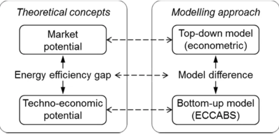
This work compares estimates of the market potentials for energy savings derived using a top-down model that employs decomposition and econometrics with estimates of the techno-economical savings potentials obtained using a bottom-up strategy comprising a building physics-based model (Energy, Carbon and Costs Assessment for Building Stocks [ECCABS]; Mata et al., 2013a) that applies a social discount rate. In the above-mentioned taxonomy described by Swan and Ugursal (2009), the top-down model is of the econometric variety and the bottom-up model is of the engineering archetype variety. Two scenarios on energy prices which differ only in the carbon tax component of each are used as inputs for both models. These price scenarios are based on the 450-ppm scenario of the 2009 IEA World Energy Outlook (IEA, 2009). The methodological framework is shown schematically in Figure 1. It is clear from the figure that the difference in estimated savings potentials calculated from the top-down and bottom-up models represents a proxy for the magnitude of the energy efficiency gap.
Figure 1 : Methodological framework applied in this work. The left panel illustrates the theoretical concepts, and the right panel outlines the corresponding modelling approach.
The present analysis was conducted for the Swedish residential housing stock that existed in 2005, i.e., dwellings constructed or demolished in or after Year 2006 are not included. The reason for this is that speculating about construction and demolition rates to Year 2030 would add a layer of complexity to the modelling, which would not enhance the aim of exploration of the efficiency gap. As it happens the construction rate in Sweden has been less than 0.5 % per annum between 1990 and 2005 meaning that the addition of new dwellings would take many years to have a large effect on energy demand. In addition, the present work involves estimations of the useful energy demand savings potentials in both models, rather than the final (delivered) energy demand savings potentials. This is the case because the influence of fuel switching on energy demand for space and water heating observed in Sweden
between 1970 and 2005 is not expected to continue at the same pace, and for a study that has more of a methodological focus, it is desirable to have one less parameter of uncertainty.
6
2.1 Top-down econometric model
The market potential for energy savings for the existing stock to Year 2030 is calculated using
decomposition and econometrics. Thus, energy demand for space and water heating, Et, is decomposed
into three sub-components (IEA,1997; Appendix 1):
(1)
where E is the useful use of energy for space and water heating (measured in TWh), A is the population in millions,
S is the residential sector floor area per capita (measured in m2),
I is the unit consumption of useful energy for space and water heating (measured in kWh/m2), and t is time in years
To estimate the value of Et for the existing stock to Year 2030, At and St are locked at the 2005 levels,
while future estimations of It to Year 2030 are used. The unit consumption for energy use for space and water heating defined above as ‘I’, It, is calculated from:
2
where P is the weighted average price for energy for a year (in SEK/toe2),Y is the annual income per capita (in SEK), t is the time (in years) and includes autonomous technical progress, HDD is the heating degree days, α is the short-term price elasticity of demand for I, β is the short-term income elasticity of demand for I, γ is the coefficient of the previous year’s I (lagged demand), δ is the coefficient of heating degree days, ε is the exponential time trend coefficient, C is a constant, and e
represents the model residuals. The values of α, β, γ, δ, and ε are calculated from time series data from 1970 to 2005 using regression analysis software. The use of the log-log regression form means that α is the price elasticity of demand for I. The use of the exponential trend means that ε times 100 is the percentage change per year in unit consumption due to various factors, such as autonomous
technological development, imposition of regulations, and additional variables not captured by price, income, lag, and HDD.
Changes in future useful energy demand for space and water heating in the existing stock will occur due to changes in unit consumption3, I. The factor I is an established indicator of progress with energy
efficiency, although the effects of conservation, changing habits, and the climate will also obviously 2 The energy prices and personal income levels must be in the national currencies, in the present case SEK, as householders would have reacted to the dynamics of the currency. However, for comparison purposes, the energy price data are presented in Euro in Table 1 below. 1
cause it to change. Increases in energy prices (P), regardless of whether they are due to market developments or the imposition of carbon taxes, should in theory lead to decreases in unit
consumption. In practice, this means that if energy prices increase and a home owner or tenant wants to reduce their energy bill, they can decrease the indoor temperature, shorten the duration of home heating or reduce their use of hot water. These are short-term responses to price changes and are captured by the short term price elasticity (α). Increases in income, as captured by term β, can at the same time lead to increased use of energy services, e.g., higher indoor temperatures, and may even offset the effect of price increases. Combining the coefficient of the lag operator It-1, γ, with α produces the long-term price elasticity [α/(1- γ)], and combining γ with β produces the long- term income elasticity [β/(1- γ)], which reflects these effects.
Coefficient δ accounts for the historic influence of climate (as represented by HDD) on demand. This is important to capture in the case of space heating, as colder winters inevitably lead to higher demand for space heating as can be seen in in Figure 2c.
In the long run, there are also technical improvements that improve the efficiency of energy use, regardless of price and income dynamics. These technical improvements may occur as a result of stricter efficiency standards and/or due to autonomous technical breakthroughs. As these
improvements are typically implemented during the renovation cycle of a building, they only occur in a fraction of the building stock in any given year. Nonetheless, these trends may be important in the long term, and therefore they are incorporated into Equation (2) using the term ε. In practice, long-term technical trends are represented by the time variable t, and this variable also includes the influence of other variables that are not captured by prices, income, lagged demand, and HDD. To calculate It for Year 2006, It-1, which is It for Year 2005, should be used. However, as the It for 2005 acts as a seed for Equation (2) and influences future outputs, the space heating component of this value is first normalised for climatic influences. For the scenarios, the coefficient of HDD, δ, is suppressed, since its role is to establish realistic price and income elasticities rather than to influence future demand patterns. For these two reasons and to ensure that the first data-point estimated (2006) from the model is aligned with measured climate-corrected useful energy demand data (2005), the model constants are adjusted accordingly.
3 As stated previously, the present work assumes a constant floor area for the model period, i.e., no
8
Figure 2 : Time series data used in this study. a, Measured space and water energy demand by energy carrier. b, Measured unit consumption of both final and useful energy demand. c, Indices of measured demand, price,, income and HDD. d, Measured prices and incomes, as well as estimated prices and incomes for the scenario period 2006–2030. El D = Direct electric heating, Wood U = Unprocessed wood, El HP = Heat pump electricity.
The time series for Equation (2), which were obtained from the IEA (2008), Odyssee Database (2009), Schipper, (2010) and other Swedish sources, are shown in Figure 2. In energy carrier mix presented in Figure 2a oil; district heating; electricity; and unprocessed wood stand out as the dominant energy carriers. Figure 2b shows unit consumption for useful energy demand. This is calculated by multiplying the final energy use for each individual energy carrier shown in Figure 2a by their respective conversion efficiency and then dividing total useful energy demand by total floor area for the residential sector . Conversion efficiencies have been published by the Swedish National Board of Housing, Building and Planning [Boverket, in Swedish] (NBHBP, 2009) for the existing residential stock in Sweden for Year 2005. No older data were found to be available. The national average conversion efficiencies for district heating (DH) and electricity in Year 2005 are both 98% (ibid.) and are assumed to be static throughout the time period of 1970–2005. The national average conversion efficiencies for oil and unprocessed wood in Year 2005 are 85% and 70%, respectively (ibid.). These efficiencies are also assumed to be static between 1970–2005 for the following reasons: There have been some minor improvements in the levels of efficiency of combustion of oil and wood for home space and water heating in Sweden since the pre-oil crisis era. However, the ways in which such boilers have been used have had far greater impacts on the efficiency of their operation. For oil-fired
0 20 40 60 80 100 1970 1975 1980 1985 1990 1995 2000 2005 TW h
Oil El D DH Wood U El HP Wood P Gas Coal
0 70 140 210 280 350 1970 1975 1980 1985 1990 1995 2000 2005 Ind ex 1970 = 100
Useful Energy Demand Price Income HDD
0 50 100 150 200 250 300 350 1970 1975 1980 1985 1990 1995 2000 2005 kW h/ m 2/y ear
Useful Energy Demand
0 5000 10000 15000 20000 25000 0 20 40 60 80 100 120 140 160 1970 1980 1990 2000 2010 2020 2030 €2005 /C a p it a €2005/ M W h
Price Low Price High Price Income Income Scenario
Measured data
Scenario data
a c
boilers the quality of heat exchangers and whether the boiler is located in a house cellar or outside the house are greater determinants of their heat supply. The heat loss from a boiler located in a cellar can also for example dry clothes. For wood-burning stoves the use of shunt valves and large accumulator tanks has a far greater impact on the amount of fuel used than the actual efficiency of the stove. In addition the condition of the wood itself (i.e., how dry it is) and the ease of access to the wood (i.e., if one owns the forest or not) are also of more importance than the actual conversion efficiency. The range of uncertainty surrounding values for the useful heat contribution of oil and wood based boilers suggests that from a modelling point of view the most accurate solution is to keep the values constant using the data available for 2005 (Thunman, 2014). The efficiency of a proportion of the electricity used for space heating is assumed to increase starting in Year 1997 due to the increased penetration of heat pumps4. The index values shown in Figure 2c reveal how energy demand has increased in cold years (as represented by HDD values), while energy prices have increased by more than 200% over the same period. Figure 2d shows the price and income data for the period 1970–2005 and two distinct price scenarios and one income scenario for the period 2006–2030.
Future estimations of energy price levels are also needed to calculate the unit consumption, I, in Equation (2). These estimations are described in Section 2.3. Income per capita is set to increase by 1.98% per annum (EC, 2008). The time series were tested for stationarity and cointegration using the Augmented Dickey-Fuller test (ADF). The tests revealed that the time series for HDD were stationary, whereas the time series for price and income were non-stationary. It was also found that the time series for demand, price, income, HDD, and time trend were cointegrated, which means that the coefficients obtained from an Autoregressive Distributed Lag (ARDL) regression model (as in Equation (2)) should be valid. The multicollinearity of the explanatory variables used in Equation (2) was checked by calculating the variance inflation factor (VIF) for each of the explanatory variables. Although the results show the presence of multicollinearity with trend and lag, it is assumed that this does not negatively affect any of the scenario results. Serial correlation of all regression errors was examined by calculating the Durbin h statistics. Heteroscedastic robust standard errors were used to calculate the t statistics (Table 2).
2.2 Bottom-up engineering building stock model
The ECCABS model (Mata et al., 2013a) applies a portfolio of technical energy saving measures (ESMs), which are chosen to exploit the savings potential, to a set of sample buildings, i.e., the energy demand of individual buildings is calculated based on the physical properties of the buildings and their
4 From 1997 to 2005, electricity use for space and water heating is divided into that which is used to power
heat pumps and that which is used for direct heating. This is done using data on the number of dwellings that have heat pumps installed (Svenska Värmepumpföreningen, 2013). For this category, useful energy for space
10
levels of energy use. In all, 1400 sample buildings, representing the Swedish residential building stock that existed in Year 2005, are modelled in this paper. Data for the sample buildings were obtained from the so-called BETSI program (Tolstoy, 2011), in which NBHBP (2009, 2010) in cooperation with Statistics Sweden [Statistiska centralbyrån (SCB), in Swedish] chose sample buildings that were statistically representative of the Swedish residential building stock. The number of buildings
corresponds to 300 categories that combine building design, age, and location (Hjortsberg, 2011). In addition, the average power demand for hot water production and the average electricity demand for lighting and appliances (in W/m2), which are required in the model as an input (in W/m2), were taken respectively from the Swedish Energy Agency (2009, 2011). See Mata et al. (2013b) for further details of the model inputs used to describe the Swedish residential building stock.
The results for the sample buildings are scaled-up to represent the entire building stock of a region or country. The calculated net energy for end-uses for the building stock is converted into final energy using conversion efficiency factors for the fuels used. The potential reductions in energy demand are calculated with respect to a baseline or reference year (Year 2005 in this work), which represents the current state of the existing building stock (the energy use in this reference year is described in Section 2.3). The energy demand reduction shown to be profitable relative to the reference year is the techno-economical energy savings potential.
In the model, an ESM is considered to be cost-effective when the cost saving obtained through applying the ESM exceeds the total cost for the ESM. The cost of the ESM includes the direct costs, i.e., initial investment costs for materials, labour, and installation required to apply the measure over its entire life, as well as the maintenance and operational costs. Indirect costs, such as the costs for policy implementation and the costs for consumer information programmes, are not considered. Regarding the cost saving obtained by applying the ESM, this is the cost of the unused (conserved) energy based on the energy prices scenarios used as input to the model, and is discounted to the starting Year 2005. A discount rate of 4% has been assumed (Mattsson, 2011), which is a typical social return rate for business. The total energy saving potential per ESM is the same in both scenarios examined, and is listed in Table 3 based on the findings of Mata et al., (2013b). See Mata et al. (2014) for further details on the cost calculations within the ECCABS model.
In total, nine types of ESMs5, outlined in Table 3 and in Section 3.2, are assessed, and they can be assigned to four categories:
and water heating is assumed to be 1.35‐times the level of input electricity (Profu, 2013).
5 As useful energy use is examined in this paper the terms energy saving measure and energy conservation
the retrofit of the different parts of the envelope, i.e., basement, façade or roof (measures 1 to 3, respectively), and the replacement of windows (measure 4);
the use of ventilation systems with heat recovery for single-family dwellings (SFD) (measure 5) and for multi-family dwellings (MFD) (measure 6);
a reduction in the use of hot water for SFD (measure7) and for MFD (measure 8) through substitution of the existing water taps with aerator taps;
a 1.2°C reduction of the average indoor temperature down to 20°C through the installation of thermostats (measure 9).
Since the aim is to calculate techno-economical potential savings, we assume that the ESMs are fully applied, i.e., that the technology is installed and operated correctly in each case. Direct or indirect rebound effects from the implementation of ESMs are not taken into consideration. These two assumptions are of course a simplification, as the ESMs are dependent upon correct operation by the occupants and in some cases, behavioural changes, for instance that occupants are willing to cope with reduced indoor temperatures.
2.3 Future energy prices
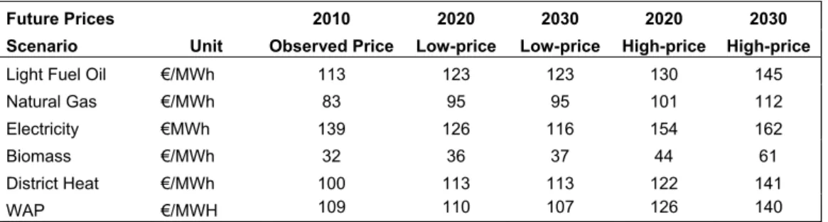
Two scenarios of future energy prices from Year 2006 to Year 2030 (Table 1) are used as input parameters to both the top-down model described in Section 2.1 and the bottom-up model described in Section 2.2. In both price scenarios, actual market prices are used (OPEC, 2010, BAFA, 2010) for the period 2006–2010, and price estimates are used thereafter. The reason why two price scenarios are chosen is to distinguish between the case in which no price-induced efforts towards CO2 mitigation occur (low-price scenario) and the case in which they do occur (high-price scenario). Although such a distinction is not necessary for the main purpose of the paper, i.e., comparing the results from two alternative models, it nonetheless ensures the robustness of the results.
For the bottom-up model, the price scenarios needed as model inputs are the full price including taxes paid by householders for each of five common energy carriers used for space and water heating. Coal is excluded, as it is rarely used for home heating in Sweden. For the top-down model, a weighted average price (WAP) for the same five energy carriers is generated. This is done by combining the prices for the five energy carriers with the IIASA GAINS baseline projection for demand (IIASA, 2010) for the same energy carriers.
The only difference between the two scenarios is that in the low-price scenario, carbon taxes are assumed to continue at the Year 2005 rate, while in the high-price scenario, carbon prices rise to €80 per tonne CO2 by 2030. This means that the commodity prices for oil, coal, and gas are the same in both scenarios. The justification for making this assumption is that although oil prices fall in the
high-12
price scenario as a result of demand, in the low-price scenario a ceiling is placed on oil price rises by the increased supply of coal to liquids. The basis for the prices is the IEA WEO 2009 “4506” scenario (IEA, 2009) for future oil, natural gas, and coal prices for Years 2020 and 20307. In the WAP, for the low-price scenario shown in Table 1, the price actually falls. This is a result of the influence of the falling electricity price in the low-price scenario and is a similar development to that used in the reference price scenario of a recent EC analysis of energy prices and costs in Europe (EC, 2014).
Table 1 : Energy prices scenarios for residential sector customers to Year 2030, as used in this work.
Future Prices 2010 2020 2030 2020 2030
Scenario Unit Observed Price Low-price Low-price High-price High-price
Light Fuel Oil €/MWh 113 123 123 130 145 Natural Gas €/MWh 83 95 95 101 112 Electricity €MWh 139 126 116 154 162 Biomass €/MWh 32 36 37 44 61 District Heat €/MWh 100 113 113 122 141 WAP €/MWH 109 110 107 126 140
A two-step process is used to transform the IEA prices, which are those for the energy carriers as traded commodities, to household prices. First, a price model, ENPAC (Axelsson and Harvey, 2010), takes the commodity prices for oil, natural gas, and coal and calculates the industrial wholesale prices for the same energy carriers, as well as for electricity, DH, and biomass. Second, carbon tax,
distribution charges, excise tax, and VAT are added, to obtain the household prices. The data for the latter three parameters are obtained from historical price data available from the IEA (2009a), which are assumed to continue along historical lines after Year 2010. In the case of distribution charges, these are assumed to be the average historical difference between the industrial wholesale prices without taxes and the household prices without taxes, and they are found to increase costs by 10%– 60%, depending on the energy carrier in question. Thereafter, the two carbon prices are applied to differentiate the scenarios. These variable CO2 charges are adopted from Axelsson and Harvey (2010), who have designated these levels as representing a business-as-usual approach in the low-price
scenario and a high mitigation policy framework in the high-price scenario. It can be argued that a carbon tax of €80 per tonne CO2 by 2030 is still low, given that the carbon tax in Sweden in 2005 was >€100 per tonne CO2. However, due to exemptions, this tax in Sweden is for the most part applied to the use of home heating oil. An investigation of the effect on the results for oil of a carbon tax of €100 per tonne CO2 in Year 2005 revealed a negligible effect due to the limited use of home heating oil. Thus, the current level of CO2 tax in Sweden was not taken into consideration; instead, the prices 6 As the name suggests, the 450 scenario is one in which the concentrations of greenhouse gases in the atmosphere are stabilised at 450 ppm of CO2equivalent by Year 2030. 7 As the WEO data are given in US dollars, it is first converted to Euro for use in the ENPAC model and then to SEK for modelling purposes using the exchange rates for Year 2005.
derived from modelling focused on the EU Emission Trading Scheme (ETS) were used (Axelsson and Harvey, 2010).
In addition to the use of the low-price and high-price scenarios, a sensitivity analysis was carried out in which prices were maintained at Year 2005 levels up to Year 2030 and in which prices were increased by annual increments of 0% to 5% to Year 2030. Although more extreme annual price changes than those in the studied range have been observed between 1970 and 2005, e.g., 46%
increase between 1974 and 1975, 23% increase between 1979 and to 1980, and 12% decrease between 1985 and 1986, such changes have not re-occurred over the period studied, which means that a
sustained 5% annual increase in prices between 2010 and 2030 is an extreme scenario in itself.
2.4 Calibrating modelling methodologies
Both models were used to estimate the demand for space and water heating for the period 2006–2030. This was performed with each model for the two different price scenarios described above. Each model has model-specific inputs for the scenarios, such as future levels of income in the case of the top-down model and discount rates and costs of measures in the bottom-up model. Year 2005 demand for both models is 74 TWh of useful energy. This value is obtained from the ECCABS model and is similar to the statistically measured value of Final Energy Demand of 72 TWh (Odyssee Database, 2009). The level of penetration of heat pumps in Sweden in this year means that the values of useful and final energy demand are almost equal (NBHBP, 2009).
3. Results
In Section 3.1, an estimation of the market potential made using top-down modelling is presented. Section 3.2 does the same for the techno-economical potential estimated by bottom-up modelling. The difference between the results from the two models, i.e., the energy efficiency gap, is presented in Section 3.3. This is followed by a description of the role of a number of key modelling parameters.
3.1 Market potentials
Results for the market based potential are predicated on the model coefficients α to ε and the constant calculated from Equation (2). These values are listed in Table 2. All the coefficients are found to have the expected sign. The coefficients of price, HDD, and lag (α, γ, ε) are significant at the 5% level, the coefficient of the time trend trend (β) is significant at the 10% level, while that of income (γ) is not significant. The R2 and F statistics confirm the joint significance of the five explanatory variables. The residuals from the model, et, in Equation (2), are found to be cointegrated at the 5% level, which
indicates that the model is a valid representation of demand. The value for α (short-term price elasticity) of -0.15 is relatively low and inelastic. The long-term price elasticity is -0.29, which is calculated by taking the effect of the lag (β) into consideration, and it is also inelastic. VIF tests show
14
multicollinearity between the lag and time trend, suggesting that their coefficients are biased. However, this is not considered to affect the forecasts of unit consumption (Gujarati, 2006). The calculated elasticities are similar to those obtained by Haas and Schipper (1998) and Nässen et al. (2008). Nässen et al. (2008) found short-term price elasticities of -0.07 for multi-family dwellings and -0.21 for one and two family dwellings for Sweden between 1970 and 2002. The α-value of -0.15 calculated in the present work for the entire stock of dwellings lies almost exactly between these two previously obtained values. Haas and Schipper (1998) calculated a short-term price elasticity of -0.11 for the period 1970–1993; their work was for total energy use in households. Given the difference in the number of data-points in their work and in the present study, the results are very similar. The income elasticity calculated as 0.00091 is very low and indicates nearly no impact on demand for the energy services of space and water heating with increased income. The coefficient of HDD, δ,
indicates increased demand with lower temperatures, as expected. The coefficient of the time trend, γ, which includes autonomous technical progress, indicates a decrease in demand of 0.44% per annum, regardless of the dynamics of the other explanatory variables.
Table 2 : Results for the regression of unit consumption (useful energy demand) for the components of Equation (2)a.
Coefficient t-statistic Variable VIF ADF Statistic
It (Useful Demand) 1.40
Constant 12.58
α (Price) -0.15 3.00 Pt (Price) 6.58 1.88
β (Income) 0.00091 0.01 Yt (Income) 5.94 0.30
γ (Time trend) -0.0044 1.77 t (Time trend) 17.71
δ (HDD) 0.000080 3.34 HDDt 1.33 3.63
ε (Lag) 0.47 3.37 It-1 (Lag) 20.06
et (Residual) 2.92
Mean VIF 10.32
Long-term Price elasticity -0.29 Adjusted R2 0.97 F-stat for Durbin h test 1.46
Long- term Income elasticity 0.0017 F-test statistic 191 Degrees of freedom 28
aSerial correlation is not found using the Durbin h statistic test. A Variance Inflation Factor (VIF) ≥10 is taken to indicate the presence of
multi-collinearity. The 1%, 5%, and 10% MacKinnon critical tau values for the Augmented Dickey-Fuller (ADF) unit root test of stationarity are -4.067, -3.46, and -3.2447, respectively (Gujarati, 2006). The 1%, 5%, and 10% Engle and Granger Critical tau values for the ADF test of cointegration are -2.5899, -1.9493, and -1.6177, respectively (Gujarati, 2006).
3.2 Techno-economical potentials
The results for the techno-economical potentials derived from the implementation of the nine measures are listed in Table 3. The right-most column shows the total technical potential Energy Saved (ES) for space heating and hot water for each measure (% of the baseline demand). Of note is the large
contribution to the overall savings potential of two measures: ventilation with heat recovery in SFDs and the use of thermostats to reduce indoor temperatures down to 20ºC. One qualification of the potential shown in the latter measure is that decreasing the indoor temperature, despite its great
potential for savings, is difficult to implement in less-energy-efficient houses owing to the requirement for a higher air temperature to compensate for other factors in the operative temperature (i.e., high air
velocity due to infiltrations or low radiation temperatures from the envelope surfaces). In addition, the installation of heat recovery systems usually requires improvement of the air-tightness of the building envelope (which has not been taken into account in this work), so as to maximise its efficiency. Thus, these two high-impact measures are best combined with other measures, such as changes in U-Values and replacement of windows, which increase efficiency and reduce infiltration. Figure 2 shows that 24 TWh of the potential listed in Table 3 is already available in Year 2010 (using actual market prices) and 26 TWh is available in Year 2020 (in the low-price scenario). Other studies that included
examinations of the savings potential for space and water heating in the Swedish residential sector have reported results in the same range (BFR, 1996; Dalenbäck et al.2005; Göransson and Pettersson, 2008; SOU:2008 125).
Table 3 : Cost‐effective potential saving per measure for the period 2010–2030 for the Swedish dwelling stock, expressed in TWh/yr as well as technical potential Energy Saved (ES) in % of the baseline demand.
Measure description Cost-effective potential ES (%) low-price High-price
Total 25.1 31.6 34.0%
Change of U-value of cellars/basements 0.5 0.9 0.6% Change of U-value of façades 1.6 2.3 2.1% Change of U-value of attics/roofs 1.1 1.5 1.5% Replacement of windows (U-value) 1.3 2.0 1.7% Ventilation with heat recovery, Single Family Dwellings (SFD) 6.1 9.0 8.3% Ventilation with heat recovery, Multi Family Dwellings (MFD) 0.5 0.9 0.7% Reduction of power used for the production of hot water to 0.80 W/m2(SFD) 1.1 1.7 1.5%
Reduction of power used for the production of hot water to 1.10 W/m2(MFD) 0.2 0.2 0.3%
Use of thermostats to reduce indoor air temperature by 1.2ºC down to 20ºC 12.8 13.1 17.2%
3.3 Quantification of the energy efficiency gap
Figure 3 gives the estimates of the energy savings obtained from the top-down (market potential) and bottom-up (techno-economical potential) modelling presented above. Figure 3a shows the
development of the energy efficiency cap in the low-price scenario in the period 2005–2030 while Figure 3b compares the results from the low-price and high-price scenarios for Year 2030.
The market savings potential in Year 2030 is 17 TWh (23%) in the low-price scenario, as compared to the level of demand in Year 2005. In the high-price scenario, the corresponding savings potential is 21 TWh (28%). The techno-economical savings potential in Year 2030 is 25 TWh (34%) in the low-price scenario, as compared to the level of demand in Year 2005, while in the high-low-price scenario the corresponding savings potential is 32 TWh (43%). The differences in the savings potentials to Year 2030 between the models i.e. the energy efficiency gap, are 8 TWh in the low-price scenario and 11 TWh in the high-price scenario.
16
Figure 3 : Estimates of energy savings obtained from the top‐down (market potential) and bottom‐up (techno‐ economical potential) modelling of this work.
It is clear from the data in Figure 3a that the market savings potential from the top-down model follows historical trends in demand (i.e., a linear continuation of the demand profile from 1970 to 2005), while the bottom-up model, metaphorically speaking, takes a sweep through the entire building stock and implements the cost-effective savings opportunities that it finds. This explains why there is a step-change in demand (from 74 TWh to 54 TWh, i.e., a cost-effective potential of 20 TWh) in 2005 for the techno-economical potential (Figure 3a). It can thus be observed that the time dimension is of less importance in the bottom-up model, as four-fifths of the techno-economical potential for Year 2030 is available in the first year of the scenario period. A further techno-economical potential of 5 TWh to Year 2030 occurs as a result of energy price increases and discounting over the period. The top-down model on the other hand requires a time dimension to reduce the gap to the
techno-0 10 20 30 40 50 60 70 80 2005 2010 2020 2030 TWh Low‐Price Market Potential Low‐Price Techno‐economical Potential 0 10 20 30 40 50 60 70 80 Low‐Price 2030 High‐Price 2030 TWh Market Potential Techno‐economic potential Reference year demand (2005) = 74 TWh 11 TWh gap 8 TWh gap 8 TWh gap a b Reference year demand (2005) = 74 TWh 17 TWh 25 TWh 13 TWh 18 TWh 20 TWh
economical potential savings that the bottom-up model shows to be possible. Because of this, the gap between results from both models decreases with time from 20 TWh in 2005 to 8/11 TWh in 2030. This can also be interpreted as arising because there are no barriers to the deployment of ESM’s included in the bottom-up model whereas the time taken to overcome barriers is implicit in the top-down model. It can also be observed data in Figure 3b that increasing prices (from the low-price to high-price scenario) lowers demand in Year 2030 in both scenarios by between 5% and 9%, as compared to Year 2005, and also increases the size of the gap by 2 TWh.
An energy efficiency gap of 13 TWh for 2016 was estimated for space and water heating in Swedish dwellings in a public enquiry published in 2008 (SOU:2008 125). This is the same as the gap of 13 TWh estimated in the present work for 2020 for the low-price scenario (or slightly below the 14 TWh estimated for the high price scenario). The 13 TWh gap calculated in the public enquiry is the
difference between a techno-economical savings potential of 17 TWh and savings of 4 TWh that are expected from autonomous technical progress and efficiency policy already in place. Although the savings potentials calculated in this work for 2020 are larger than those calculated in the public enquiry for 2016 it is interesting that the same magnitude of gap has been obtained in both studies. Nonetheless the energy efficiency gap found in the present study and in the public enquiry are small compared to total energy demand, e.g., 8/60 (cf. Figure 3a) = 13 % in the low-price scenario. This may be because much has already happened to improve efficiency in the Swedish residential sector since the oil crises.
3.4. Key modelling parameters
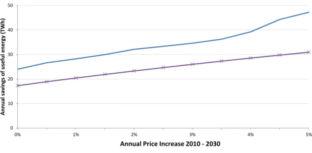
The results from the two models are heavily influenced by the key modelling parameters, which include energy prices, the time trend, the number of ESMs considered, and the discount rates applied. The role that energy price changes play in the models has been examined in a sensitivity analysis using scenarios of price changes from Year 2010 to Year 2030 in 0.5% increments, from 0% per annum to 5% per annum8. The results of the analysis for Year 2030 (Figure 4) show that the difference in annual savings of useful energy in Year 2030 between the market potential and the
techno-economical potential will range from 7 TWh for no annual increase in the price of energy to 16 TWh for an annual increase in energy prices of 5%. As expected, both models show that as energy prices rise, the savings potentials increase. For energy price increases in the range of 0%–3.5%, there is a consistent difference of approximately 8 TWh in annual savings of energy between the two models. Thereafter, the gap in energy savings increases as more technological measures become cost-effective in the bottom-up model. Thus, from the methodogical point of view, the data in Figure 4 reveal that
18
the two models have similar sensitivities to energy prices up to an annual price increase of 3.5%, which over a 20-year period (2010– 2030) would correspond to an energy price increase of approximately 100%.
Figure 4 : Sensitivity analysis of estimates of energy savings potentials in Year 2030, as obtained from the top‐down (market potential) and bottom‐up (techno‐economical potential) modelling of the present work over a range of annual price increases (0%–5%).
It might be argued that the use of a WAP for energy in the top-down model, in contrast to the use of prices for individual energy carriers in the bottom-up model, creates a calibration issue of relevance to any comparison of the results from the two models. However, when different future weights for the energy carriers were tested the results were not changed by more than 0.5 TWh, which means that this is not an issue.
The coefficient of the time trend variable of the top-down model, γ in Equation (2) and in Table 2, shows historic savings of 0.44% per annum, regardless of the dynamics of price and income and the other explanatory variables (see Table 2). In the low-price scenario, for example, it is the magnitude of
γ that causes demand to fall, despite the fact that prices also fall in this scenario. However, the market potential calculations are based on the time trend of the entire stock of residential buildings, which in addition to energy efficiency improvements in existing buildings has also been affected by the addition of new buildings with higher energy efficiencies than the average stock in the period from 1970 to 2005. This may have resulted in an overestimation of the market potential to Year 2030, given that similar construction rates cannot reasonably be expected in future decades. Therefore, our estimate of 8 The average annual price changes for the low‐price and high‐price scenarios used in the present work are ‐0.3 % and +1.1 %, respectively. 0 10 20 30 40 50 0% 1% 2% 3% 4% 5% Annua l sa vi ngs of u se ful en er gy (TWh ) Annual Price Increase 2010 ‐ 2030 Techno‐economical Potential 2030 Market Potential 2030
the gap between the results from the top-down and bottom-up models may also be slightly underestimated.
For the techno-economical estimates, the cost-effectiveness of the ESMs is very sensitive to the discount rates used in the calculations, even for values considered to be within the meaning of a ‘social discount rate’. Applying discount rates in the range of 1% to 6%, in which the lower rates represent policy actions that facilitate investments in ESMs by offering low interest loans, while 6% is the additional discount rate that the EC recommends for the financial calculations in the EPBD-related reporting of the cost-optimal levels of energy performance (NBHBP, 2013), has significant effects on the net annual costs of the ESMs (cf. Figure 4 in Mata et al., 2014).
The number of ESMs considered in the bottom-up model is of course a determinant of the size of the energy efficiency gap. For the purposes of the present work, the results are valid for the portfolio of measures applied. For the first of the four categories of measures listed in Section 2.3, accurate assessments of techno-economical savings potentials are possible because the relevant physical characteristics of the sample buildings are known. The modelling shows that 80% of the buildings have undergone renovation of at least one of the four compartments of their envelope. For the other three categories of measures listed in Section 2.3, there may be some overestimation of the techno-economical savings potentials as some buildings may already have undergone improvements (e.g., aerator taps installed) that are not included in the building description database used (Mata et al, 2013b). Finally, the ESMs are modeled individually and not simultaneously (Mata et al, 2013a), which results in a possible underestimation of the potential energy savings obtained from the bottom-up modeling because possible synergies between the measures are not taken into account.
4. Discussion
The results obtained from the two models are of relevance to policy makers, with the caveat that there is a clear understanding of the assumptions made and of the corresponding limitations and strengths of the present work. In other words, the bottom-up model indicates which techno-economical potential savings are available under certain assumptions regarding the costs of the ESMs, while the top-down model predicts what the outcome will be if macroeconomic forces continue along historical lines. Therefore, interpretation of the results of the present study from a policy perspective is warranted. The results from the top-down model show the price elasticity of demand and the effects of non-price-related legislation and technical developments. Increasing energy prices as a policy measure, as implemented in the high-price scenario of this work, does not lead to significant additional savings, as shown by the top-down model. The combination of the high-price scenario and long-term price
20
elasticity of -0.29 would result in a gain (increased market potential over the low-price scenario) of only 4 TWh by Year 2030.
From the policy perspective, the step change in demand, which results from the bottom-up model show to be feasible in 2005 (see Figure 3), is unlikely to occur so quickly. This is because the bottom-up model does not include delays in the implementation of the technical changes brought about by consumer preferences, risk aversion, up-front investment costs, and asymmetric information provided to householders; these issues are not reflected in the discount rate used. However, the top-down model cannot account for the non-linear or step changes in the diffusion of efficient technologies that would be required to achieve the potential savings indicated in the bottom-up model. This raises the
following question: What level of annual savings is necessary to achieve the techno-economical potential by 2030? Using the two models in tandem, this question can be answered by calculating the value of γ in the top-down model and the discount rate in the bottom-up model that would be
necessary to close the energy efficiency gap. These two parameters represent components that are present in one model but not in the other.
If the value of γ calculated for the time trend was to increase from 0.44% per annum to 0.9% per annum ceteris paribus, the outcome from the top-down model would be the same as that from the bottom-up model by Year 2030. Therefore, attaining the techno-economical potential within this time span would require a more than twofold increase in the historic rate of support for technology
diffusion and conservation through, for example, support schemes and regulations. This could be facilitated by the implementation of the technical measures listed in Table 3, and could occur at a planned pace though the introduction of compulsory renovation rates. Furthermore, it could be facilitated by tackling the market failures component of an energy efficiency gap of 8 TWh. In this context, Karlsson (2013) shows that the Swedish Energy Agency has adopted a strategy for addressing market failures in terms of educating key stakeholders, such as property owners and banks, as to the benefits of energy-efficient building renovations.
Koomey (2000) however criticises the heavy reliance on statistically-derived historical parameters for modelling, e.g., γ in Equation (2) and in Table 2. He writes that ‘creating a world with vastly lower carbon emissions presupposes massive behavioural and institutional changes that render past relationships between energy use and economic activity largely irrelevant (just like after 1973)’. Related to this view, Sanstad and Greening (1997) write that, ‘economic models (e.g., the market potential estimated in this paper) at their best are probably only good representations of economic conditions five to ten years into the future’. With this in mind, the policy measures in place in Sweden that have resulted in the value of γ in Equation (2) have been examined. These are obtained from the MURE Policy Database (Isis, 2014) which lists twelve policies for the household sector in Sweden
and includes a semi-quantitative impact assessment of their impacts (i.e., whether they are expected to have a low, medium or high impact). Of these twelve policies, eight include in their focus reducing useful energy demand for space and water heating .These eight can be divided into two groups: 1) three policies that were introduced between 1970 and 2005, i.e., the time period used for calculating the value of γ ; and 2) five policies that were or will be introduced post 2005. Whether or not the post-2005 policy measures listed amount to a doubling of the historical efficiency-focused legislation, as prescribed in this paper is unclear. In terms of the numbers of pieces of legislation in place, this doubling has occurred, although the same cannot be stated in regard to the impact of such legislation, given that no high-impact policy measures are included. At the same time, the two post-2006 EPBD-related measures have yet to be assessed. The extent to which these two policy packages lead to significant demand reductions is crucial to the achievement of the techno-economical potential described in the present paper.
Similar to the matching of the time trend parameter to the techno-economical savings potential, we can also elaborate on how much the discount rate would have to increase in the bottom-up model for the potential it generates to equal the market savings potential seen in the top-down model. The purpose of this exercise is to calculate the implicit discount rate for the case of useful energy demand for space heating in the Swedish residential sector. We show that if the discount rate used in the calculation of the annuities in the bottom-up model of 4% (social discount rate) is increased to 10 % ceteris paribus, then the techno-economical savings potential available in the bottom-up model would be equal to that of the market savings potential shown in the top-down model (17 TWh). This is shown in Figure 5, where the savings potential is plotted for discount rates of between 4% and 20%. The value of 10% can be interpreted as the implicit discount rate for energy efficiency improvements, and we can reformulate the energy efficiency gap as a “discount gap” of 6%.
These findings can be compared to older estimates in the literature. Train (1985) summarised various earlier studies of implicit discount rates and found that for energy-related investments in home retrofitting, the average values ranged from 10% to 30%. In a bottom-up modelling exercise, Nyboer (1997) used discount rates of 50% for space heating and 80% for a space heating retrofit based on a literature review, although he had also reported values as low as 6% for a shell conservation retrofit. Therefore, while the energy efficiency gap in the Swedish residential sector certainly raises some concerns regarding unutilised potentials, this discount gap is modest in comparison to the findings of these earlier studies. Once again, this may be the result of efforts implemented since the oil crises to promote energy efficiency in the Swedish residential sector, and it means that there is strong awareness among the Swedish population of the benefits of energy efficiency.
22
Figure 5 : Techno‐economical energy savings potentials obtained from the modelling in the present study for discount rates between 4% and 20%.
5. Conclusions
In the present work, we calculated the market and techno-economical energy demands to Year 2030 for space and water heating in the existing Swedish residential buildings using a top-down and a bottom-up model, respectively. The differences between the results from the two alternative models in Year 2030 are 8 TWh and 11 TWh for a low-price scenario and a high-price scenario, respectively, and this is an ex-ante quantification of the so-called energy efficiency gap. The use of the two models calibrated to the same reference year and energy demand allows calculations of both the implicit discount rate (which was found to be 10%) and the annual rate of implementation of the combined effect of support for technology diffusion, legislation, and regulations needed to realise the techno-economical potential by Year 2030 (which was found to require a doubling of the historic
implementation rate). Increasing energy prices per se do not lead to significant savings. These results support a policy approach that involves a portfolio of measures that address not only the price mechanism, but also support for the diffusion of key technologies, and stronger regulations and information to narrow further the energy efficiency gap.
References
Axelsson E., and Harvey, S., (2010). Scenarios for assessing profitability and carbon balances of energy investments in industry, AGS Pathway report 2010:EU1, Göteborg 2010.
BAFA, (2010). German Import Border Prices for Coal and Gas. http://www.bafa.de
BFR, (1996). Energieffektivisering. Sparmöjligheter och investeringar för el- och värmeåtgarder i bostäder och lokaler. Anslagsrapport A1:1996, BFR Byggforskningsrådet, Stockholm, Sweden (in Swedish).
Booth A.T., Choudhary R., Spiegelhalter D.J. (2012). Handling uncertainty in housing stock models. Building and Environment 48: 35-47. 0 5 10 15 20 25 30 1 2 3 4 5 6 7 8 9 10 11 12 13 14 15 16 17 18 19 20 TWh Savin gs (203 0) Discount Rate (%) Market potential low‐price scenario (2030) = 17 TWh Discount gap (2030) = 6 %
Dalenbäck J. O., Görasson A., Lennart J., Nilson A., Olsson D., Pettersson B., (2005). Åtgärder för ökad energieffektivisering i bebyggelse. Report CEC 2005:1,Chalmers EnergiCentrum – CEC, Chalmers University of Technology, Gothenburg, Sweden (in Swedish).
EC, (2006). Action Plan for Energy Efficiency: Realising the Potential, COM(2006)545 final.
EC, (2008). European Energy and Transport trends to 2030 — update 2007, European Commission Directorate-General for Energy and Transport. © European Communities, 2008 ISBN 978-92-79-07620-6.
EC, (2014). Energy prices and costs in Europe, The European Commission (EC), Brussels, Belgium.
Giraudet, L.-G., Guivarch, C., Quirion, P., 2012. Exploring the potential for energy conservation in French households through hybrid modeling. Energy Economics 34, 426-445.
Gujarati, D.N., (2006). Essentials of Econometrics, Mc Graw-Hill.
Göransson, A., and Pettersson. B., (2008). Energieffektiviseringspotential i bostäder och lokaler. Med fokus på effektiviseringsåtgärder 2005 – 2016. Report - CEC 2008:3, Chalmers EnergiCentrum – CEC, Chalmers University of Technology, Gothenburg, Sweden (in Swedish).
Haas, R., and Schipper, L., (1998). Residential energy demand in OECD-countries and the role of irreversible efficiency improvements. Energy Economics 20. Pp 421-442.
Hjortsberg, M., (2011). Description of the Swedish building stock using material Swedish statistical survey of 1800 buildings, Swedish National Board of Housing, Building and Planning. Available at: http://www.boverket.se/Global/Om_Boverket/Dokument/about_boverket/betsi_study/building_stock.pd f
IEA, (1997). Indicators Manual, International Energy Agency, Paris.
IEA, (2007). Mind the Gap, Quantifying Principal-Agent Problems in Energy Efficiency, International Energy Agency, Paris.
IEA, (2008). Energy Prices and Taxes Statistics. Downloaded from SOURCEOECD website July, 2008. IEA, (2009). World Energy Outlook, International Energy Agency, Paris.
IEA, (2010). Energy Technology Perspectives, Paris.
IIASA, (2010). GAINS online database. International Institute for Applied Systems Analysis, Laxenburg, Austria. Available at http://gains.iiasa.ac.at/index.php/home-page/241-online-access-to-gains
IPCC, (2007). Levine, M., D. Ürge-Vorsatz, K. Blok, L. Geng, D. Harvey, S. Lang, G. Levermore, A. Mongameli Mehlwana, S. Mirasgedis, A. Novikova, J. Rilling, H. Yoshino, 2007: Residential and commercial buildings. In Climate Change 2007: Mitigation. Contribution of Working Group III to the Fourth Assessment Report of the Intergovernmental Panel on Climate Change [B. Metz, O.R. Davidson, P.R. Bosch, R. Dave, L.A. Meyer (eds)], Cambridge University Press, Cambridge, United Kingdom and New York, NY, USA.
ISIS, 2012. MURE II Database on energy efficiency policies and measures. http://www.muredatabase.org/ Jaccard, M., 2004. Greenhouse Gas Abatement: Controversies in Cost Assessment, Encyclopedia of Energy 3:
57-65.
Jaccard, M., 2009. Combining Top-Down and Bottom-Up in energy economy models, Chapter 13 in: International Handbook on the Economics of Energy, Edward Elgar, Cheltenham, UK.
Jacobsen, H.K., 1998. Integrating the bottom–up and top–down approach to energy–economy modeling: the case of Denmark, Energy Economics 20 (4): 443–461.
Jaffe, A., Newell, R., and Stavins, R., (2004). Economics of Energy Efficiency, Encyclopaedia of Energy, Volume 2.Elsevier Inc.
Jaffe A.B, Stavins R.N., (1994). The energy efficiency gap – What does it mean?, Energy Policy Vol. 22, No. 10, 804-810.
Joskow P.L., (1995). Utility-subsidized energy-efficiency programs, Annual Review of Energy and the Environment, Vol. 20, 526-534.
Karlsson, C. (2013). Energy Efficiency, Swedish Energy Agency. Presentation given to the 6th Passive House Conference in the Nordic Countries (Passivhushorden), Gothenburg, Sweden.
Kavgic, M., Mavrogianni, A., Mumovic, D., Summerfield, A., Stevanovic, Z., Djurovic-Petrovic, M., 2010. A review of bottom-up building stock models for energy consumption in the residential sector. Building and Environment 45, 1683-1697.
24
Koopmans, C.C., and te Velde, D.W., 2001. Bridging the energy efficiency gap: Using bottom–up information in a top–down energy demand model. Energy Economics 23 (1): 57–75.
Koomey, J. G. (2000, April). Avoiding ‘the big mistake’in forecasting technology adoption. In Proceedings of the Energex Conference.
Mata, É., Sasic Kalagasidis, A., Johnsson, F., (2013a). A modelling strategy for energy, carbon, and cost assessments of building stocks, Energy and Buildings 56 pp.100-108.
Mata, E., Sasic Kalagasidis, A., Johnsson, F., (2013b). Energy usage and potential for energy saving measures in Swedish households. Energy Policy 55, 404–14.
Mata, E., Sasic Kalagasidis, A., Johnsson, F., (2014). Cost-effective retrofitting of the Swedish residential building stock: effects of energy price developments and discount rates. Submitted for publication. Mattsson, B., (2011). Costs for reducing the energy demand in the Swedish building stock according to national
energy targets, Swedish National Board of Housing, Building and Planning. Available at: http://www.boverket.se/Global/Om_Boverket/Dokument/about_boverket/betsi_study/energy.pdf Mundaca, L., Neij, L., Worrell, E., McNeil, M., 2010. Evaluating Energy Efficiency Policies with
Energy-Economy Models. Annual Review of Environment and Resources 35, 305-344.
Nordhaus, W.D. (1991). The cost of slowing climate change: a survey, The Energy Journal, Vol 12, No 1, pp 37-65.
Nässén, J., Sprei, F., Holmberg, J., (2008). Stagnating energy efficiency in the Swedish building sector-Economic and organisational explanations. Energy Policy, 36 (10) pp. 3814-3822.
Nyboer J., (1997). Simulating evolution of technology: an aid to energy policy analysis, Thesis submitted in partial fulfilment of the requirements for the degree of Doctor of Philosophy, Simon Frasier University, Canada.
Odyssee Database, (2009). http://www.odyssee-indicators.org/ OPEC, (2010). Opec Monthly Oil Report.
Persson, A., Göransson, A., Gudbjerg, E., (2008). Bridge over troubled water – Spanning the energy efficiency gap, ECEEE Summer Study Proceedings.
Profu, (2013). Beräkningar av nettovärme i redovisningsverktyget HEFTIG. Profu Consultancy, Mölndal, 43134 Sweden. In Swedish.
Rivers, N. and M. Jaccard, 2005. Combining Top-Down and Bottom-Up Approaches To Energy-Economy Modeling Using Discrete Choice Methods. The Energy Journal 26 (1): 83-106.
Sanstad, A. H., & Greening, L. A. (1998). Economic models for climate policy analysis: A critical discussion. Environmental Modeling & Assessment, 3(1-2), 3-18.
Schipper, L., 2010. Personal correspondence with author.
Sorrell, S., O'Malley, E., Schleich, J., and Scott, S., (2004). The economics of energy efficiency: barriers to cost-effective investments. Edward Elgar Publishing Limited.
SOU 2008:125, (2009). Vägen till ett energieffektivare Sverige, Statens Offentliga Utredningar. (In Swedish). Summerfield A. J. and Lowe, R. (2012) Challenges and future directions for energy and buildings research,
Building Research & Information, 40:4, 391-400.
Swedish Energy Agency, (2009). Mätning av kall- och varmvattenanvändning i 44 hushåll - Delrapport i Swedish Energy Agencyens projekt Förbättrad energistatistik i bebyggelsen och industrin, ER 2009:26 (in Swedish). Eskilstuna, Sweden.
Swedish Energy Agency, (2011). Facts and figures- Energy in Sweden 2011. Eskilstuna, Sweden.
NBHBP, (2009). Så mår våra hus. Redovisning av regeringsuppdrag beträffande byggnaders tekniska utformning m.m. (in Swedish). Swedish National Board of Housing, Building and Planning (NBHBP, Boverket in Swedish), National Board of Housing, Building and Planning, Karlskrona, Sweden. NBHBP, (2010). Energi i bebyggelsen – tekniska egenskaper och beräkningar. Resultat från projektet BETSI (in
Swedish). National Board of Housing, Building and Planning, Karlskrona, Sweden.
NBHBP, (2013). Optimala kostnader för energieffektivisering– underlag enligt Europaparlamentets och rådets direktiv 2010/31/EU ombyggnaders energiprestanda, Slutrapport Rapport 2013:2, REGERINGSUPPDRAG N2012/2823/E (in Swedish). National Board of Housing, Building and Planning, Karlskrona, Sweden.