HAL Id: hal-01136286
https://hal.archives-ouvertes.fr/hal-01136286
Submitted on 27 May 2020
HAL is a multi-disciplinary open access
archive for the deposit and dissemination of
sci-entific research documents, whether they are
pub-lished or not. The documents may come from
teaching and research institutions in France or
abroad, or from public or private research centers.
L’archive ouverte pluridisciplinaire HAL, est
destinée au dépôt et à la diffusion de documents
scientifiques de niveau recherche, publiés ou non,
émanant des établissements d’enseignement et de
recherche français ou étrangers, des laboratoires
publics ou privés.
To cite this version:
Marcel van Oijen, J. Balkovic, Christian Beer, D. R. Cameron, Philippe Ciais, et al.. Impact of
droughts on the C-cycle in European vegetation:A probabilistic risk analysis using six vegetation
models. Biogeosciences, European Geosciences Union, 2014, 11 (22), �10.5194/bg-11-6357-2014�.
�hal-01136286�
www.biogeosciences.net/11/6357/2014/ doi:10.5194/bg-11-6357-2014
© Author(s) 2014. CC Attribution 3.0 License.
Impact of droughts on the carbon cycle in European vegetation:
a probabilistic risk analysis using six vegetation models
M. Van Oijen1,2, J. Balkovi3, C. Beer4,5, D. R. Cameron1, P. Ciais6, W. Cramer7, T. Kato6,13, M. Kuhnert8, R. Martin9, R. Myneni10, A. Rammig11, S. Rolinski11, J.-F. Soussana9, K. Thonicke11, M. Van der Velde2, and L. Xu10,12
1Centre for Ecology & Hydrology, Edinburgh, EH26 0QB, UK 2Bioforsk, Saerheim, Norway
3International Institute for Applied Systems Analysis (IIASA), Schlossplatz 1, 2361 Laxenburg, Austria 4Max-Planck-Institute for Biogeochemistry, Jena, Germany
5Department of Applied Environmental Science (ITM), Bolin Centre for Climate Research,
Stockholm University, Stockholm, Sweden
6Laboratoire des Sciences du Climat et de l’Environnement, CEA-CNRS-UVSQ, 91198 Gif-sur-Yvette, France 7Institut Méditerranéen de Biodiversité et d’Ecologie marine et continentale (IMBE), Aix Marseille Université,
CNRS, IRD, Avignon Université, 13545 Aix-en-Provence, France
8University of Aberdeen, School of Biological Sciences, Aberdeen, UK
9INRA, Grassland Ecosystem Research, (UR 874), 63100 Clermont-Ferrand, France 10Department of Earth and Environment, Boston University, Boston, USA
11Potsdam Institute for Climate Impact Research (PIK), Telegrafenberg 31, 14473 Potsdam, Germany 12Institute of the Environment and Sustainability (IoES), University of California, Los Angeles, USA 13Research Faculty of Agriculture, Hokkaido University, Sapporo, 060-8589 Japan
Correspondence to: M. Van Oijen (mvano@ceh.ac.uk)
Received: 24 March 2014 – Published in Biogeosciences Discuss.: 5 June 2014
Revised: 25 September 2014 – Accepted: 23 October 2014 – Published: 26 November 2014
Abstract. We analyse how climate change may alter risks
posed by droughts to carbon fluxes in European ecosys-tems. The approach follows a recently proposed framework for risk analysis based on probability theory. In this ap-proach, risk is quantified as the product of hazard probabil-ity and ecosystem vulnerabilprobabil-ity. The probabilprobabil-ity of a drought hazard is calculated here from the Standardized Precipita-tion–Evapotranspiration Index (SPEI). Vulnerability is cal-culated from the response to drought simulated by process-based vegetation models.
We use six different models: three for generic vegeta-tion (JSBACH, LPJmL, ORCHIDEE) and three for spe-cific ecosystems (Scots pine forests: BASFOR; winter wheat fields: EPIC; grasslands: PASIM). The periods 1971–2000 and 2071–2100 are compared. Climate data are based on gridded observations and on output from the regional climate model REMO using the SRES A1B scenario. The risk anal-ysis is carried out for ∼ 18 000 grid cells of 0.25 × 0.25◦
across Europe. For each grid cell, drought vulnerability and risk are quantified for five seasonal variables: net primary and ecosystem productivity (NPP, NEP), heterotrophic respi-ration (Rh), soil water content and evapotranspirespi-ration.
In this analysis, climate change leads to increased drought risks for net primary productivity in the Mediterranean area: five of the models estimate that risk will exceed 15 %. The risks increase mainly because of greater drought probabil-ity; ecosystem vulnerability will increase to a lesser extent. Because NPP will be affected more than Rh, future carbon sequestration (NEP) will also be at risk predominantly in southern Europe, with risks exceeding 0.25 g C m−2d−1
ac-cording to most models, amounting to reductions in carbon sequestration of 20 to 80 %.
(e.g. Drake et al., 1997; Morgan et al., 2004; Keenan et al., 2013), a mechanism which could partly alleviate the sensitiv-ity of plants and ecosystems to drought. How these changes will affect the vulnerability of vegetation to future drought and the associated risks has not yet been rigorously quanti-fied (Van Oijen et al., 2013b).
Risk analysis is applied in many fields, and terminology is inconsistent (Brooks, 2003; Schneiderbauer and Ehrlich, 2004). Generally, “hazard”, “vulnerability” and “risk” are distinguished (DHA, 1992). “Hazard” refers to damaging conditions which may on occasion prevail. “Vulnerability” refers to the sensitivity of the impacted system to those dam-aging conditions. “Risk” is commonly defined as an expecta-tion value for loss induced by the hazardous condiexpecta-tions. Al-though most work on risk analysis distinguishes three such terms, the definitions – in particular of vulnerability – are generally too imprecise to place the terms in a mathematical relationship to each other (Ionescu et al., 2009). Risk analy-ses thus tend not to show how exactly risk should be decom-posed into its two constituent terms, hazard and vulnerability. This hampers the use of risk analysis to ecosystems when we are interested not only in quantifying risk, or changes in risk, but also in identifying the main causal factors. In the present study, we aim to disentangle two effects of climate change in a risk analysis framework. First, to what extent does cli-mate change lead to increased probability of extreme, haz-ardous weather? Second, how does climate change affect the vulnerability of ecosystems to such extreme conditions? For this, we require a quantitative method that allows risk to be decomposed.
Recently, we proposed a method for probabilistic risk analysis (PRA) which is able to decompose the risk into two constituent terms (Van Oijen et al., 2013b). The PRA is de-signed to analyse the effect of any environmental variable on any system variable of interest. An example could be the impact of drought on ecosystem carbon flux. The method allows for either variable to be derived from measurement or from modelling. “Hazardous conditions” are defined as those where the environmental variable is more extreme than a given threshold, and their probability of occurrence is de-noted as P (H ). We define vulnerability (V ) as the difference between the expectation values for the system variable un-der non-hazardous and hazardous conditions. Risk (R) is de-fined, as is commonly done, as the expectation of loss: the
in a human-made system and this is modelled using discrete probability distributions. This approach is not suitable for our purposes in ecology where response variables such as carbon fluxes are not binary: fluxes do not necessarily “fail” when there is a drought but can change to any given degree. There-fore our framework for risk analysis uses continuous prob-ability distributions and we define vulnerprob-ability as a func-tion of expectafunc-tion values and not discrete probabilities. We have not been able to find the PRA equations (given below in Sect. 2.5.1 and more fully in Van Oijen et al., 2013b) in the engineering literature, although of course there is conceptual similarity between the fields.
We apply the PRA framework here to the impact of droughts on vegetation in Europe, both in recent (1971–2000) and future (2071–2100) years. Our focus is on the responses of the major carbon fluxes between ecosys-tems and the atmosphere: net primary productivity (NPP), heterotrophic respiration (Rh) and net ecosystem productiv-ity (NEP). The different carbon fluxes in ecosystems are tightly linked to each other (e.g. Raich and Schlesinger, 1992; van Oijen et al., 2010), and we can therefore analyse how drought risks to carbon sequestration in the form of NEP result from risks to the other two carbon fluxes, given that NEP = NPP − Rh. In addition, we examine the primary re-sponses of soil water content (SWC) and evapotranspiration (ET), giving five system variables in total. The water vari-ables SWC and ET are included to determine whether risks to NPP are mainly due to reductions in water availability or in water use. We quantify how risks to these five variables un-der future conditions differ from the present across Europe, and proceed by inspecting the two constituent terms of risk to pinpoint the main cause of change.
We define drought using the Standardized Precipita-tion–Evapotranspiration Index (SPEI, Vicente-Serrano et al., 2010). The SPEI is a localized measure of drought: it is based for every site on the local long-term frequency distribution of precipitation minus potential evapotranspiration. The SPEI quantifies how rare a given difference of precipitation and potential evapotranspiration is, with respect to this frequency distribution. Because one aim of our analysis is to determine in which parts of Europe climate change is expected to lead to a change in the probability of drought (P (H )), we use the same reference period for the SPEI calculations for both the present and future risk analysis, choosing 1901–2010 for this
purpose. We define as droughts those SPEI values, calculated for the half-year period from April to September, which are less than −1, i.e. more than one normalized standard devia-tion below average (Sect. 2.2).
Apart from the SPEI, various other drought indices exist (Joetzjer et al., 2013). For example, the Standardized Pre-cipitation Index (SPI) is a simpler index, requiring only in-formation about the time series of precipitation at a site. In contrast to this, the often used Palmer Drought Severity In-dex (PDSI) requires extra information about soil water hold-ing capacity to allow estimation of a local water balance. The SPEI does not require such detailed information, yet ac-counts for the impact of other meteorological variables be-sides precipitation on the severity of a drought. There is long-standing and active debate in the literature about the strengths and weaknesses of different drought indices (e.g. Vicente-Serrano et al., 2010; Sheffield et al., 2012; Joetzjer et al., 2013). Much of this debate centres on whether the indices can detect whether ongoing climate change has already al-tered drought prevalence (e.g. Trenberth et al., 2014). In con-trast, our main concern here is the comparison of the impacts of recent droughts with those from expected droughts a cen-tury into the future. This period is expected to see greater changes in weather than the past century, making the choice of drought index less critical.
This paper quantifies current and future vulnerability and risk of change in major European carbon fluxes in response to drought. We present results from the PRA using six differ-ent vegetation models and discuss how the results depend on the way drought impacts are simulated. Three of the models simulate a combination of vegetation types in each grid cell, and three are ecosystem-specific (Scots pine, winter wheat, grassland). Comparison of the results from the different mod-els allows a modest assessment of the uncertainty of the risk analysis with respect to model assumptions. We evaluate the PRA using remotely sensed Normalized Difference Vegeta-tion Index (NDVI) data, and carry out a sensitivity analysis to determine the robustness of the results with regard to timing and severity of drought as well as climatic variability.
2 Materials and methods
In this section, we describe the atmospheric drivers (Sect. 2.1), the SPEI drought index (Sect. 2.2), the six mod-els (Sect. 2.3), the Normalized Difference Vegetation Index (NDVI) vegetation greenness data (Sect. 2.4) and our new method for probabilistic risk analysis (PRA, Sect. 2.5).
2.1 Climate and CO2
The vegetation models used in this study are driven with daily climate data spanning the period 1901–2100 at a 0.25 × 0.25◦longitude/latitude grid. The climate data are de-scribed in detail by Beer et al. (2014). Here, a short
sum-mary follows. For the period 1901–1978 the data set is based on WATCH forcing data (Weedon et al., 2011). For the period 1979–2010, ECMWF ERA-Interim reanalysis data are used, bias-corrected against WATCH observation-derived climate forcing data using the method described by Piani et al. (2010). From 2011 until 2100, climate data are used on the basis of outputs from the regional climate model REMO us-ing the SRES A1B scenario, with boundary conditions from the ECHAM5 general circulation model, as provided by the EU project ENSEMBLES (Hewitt and Griggs, 2004). This data set has also been bias-corrected against the 1901–2010 WATCH data set following Piani et al. (2010).
We refer to the above mentioned climate data for the pe-riod 1901–2100 as the “control climate” and most of our study will focus on the implications of climate change in-herent in that data set. Besides these control climate runs, we conducted model experiments using an additional artificial climate data set (Beer et al., 2014), referred to as the “re-duced variability climate”, which was constructed such that day-to-day and year-to-year variability of the meteorological variables are smaller than in the control while the 30-year long-term averages of annual and seasonal values are being conserved (Beer et al., 2014).
The time series for the atmospheric concentration of CO2
is based on data from ice-core records and NOAA atmo-spheric observations for the period 1901–2010 and on the SRES (Nakicenovic and Swart, 2000) A1B scenario for 2011–2100. The concentration increases from 296 ppm in 1901 to 710 ppm in 2100.
2.2 Standardized Precipitation–Evapotranspiration Index (SPEI)
To calculate time series of drought in each grid cell, we use the Standardized Precipitation–Evapotranspiration In-dex (SPEI, Vicente-Serrano et al., 2010). This inIn-dex quan-tifies the degree of drought as a function of the difference D between precipitation and potential evapotranspiration. The SPEI is a normalization of this difference, defined as the normally distributed variable (mean = 0, standard devia-tion = 1) whose cumulative probability density funcdevia-tion co-incides with that of D. The probability distribution for D is estimated from monthly data in a reference period, which we chose to be the period for which we had observational weather data, 1901–2010. With these choices, for every grid cell the average SPEI value over the years 1901–2010 is zero and about 68 % of SPEI values are between −1 and +1.
Using a long reference period, here 110 years, to calcu-late SPEI values is advisable when the focus of the study is on rare extreme events. The SPEI can be calculated for drought events of any duration, but here we only used val-ues calculated for periods of half a year. In most cases, the summer half of each year was used, from April to Septem-ber, which in Europe captures the season of highest veg-etation greenness across all latitudes (see Sect. 2.4). As a
Figure 1. Values of the SPEI drought index across Europe for the months April–September in three different time periods: (a) 1971–2000, (b) the single year 2003, and (c) 2071–2100.
Table 1. Average values of model outputs for April–September, averaged over 1971–2000. NPP is net primary productivity (g C m−2d−1), Rh is heterotrophic respiration (g C m−2d−1), NEP is net ecosystem productivity (g C m−2d−1), SWC is soil water content (mm), ET is evapotranspiration (mm d−1), and n is the number of grid cells simulated.
Model Vegetation n NPP Rh NEP SWC ET BASFOR Scots pine 11 709 3.33 2.40 0.93 364 1.86 EPIC Winter wheat 5885 2.18 0.69 1.49 77 2.15 PASIM Grassland 7756 3.76 3.20 0.56 326 1.73 JSBACH Generic 18 085 2.93 1.77 1.05 346 1.65 LPJmL Generic 17 785 2.40 1.60 0.80 69 1.27 ORCHIDEE Generic 18 075 2.57 1.35 1.22 91 1.37
sensitivityanalysis, we assessed the consequences of shifting the start of the half-year to March, February or January. The Penman–Monteith equation (Monteith, 1995) with invariant canopy conductance was used to calculate potential evapo-transpiration.
Figure 1 shows maps for the average value of the April–September SPEI in the years 1971–2000 and 2071–2100 plus an example for the European heat wave year 2003. The two 30-year time periods are the periods for which we carry out risk analysis in this paper. The SPEI in the year 2003 is shown to illustrate how a single extreme year can dif-fer from the average. 2003 had a very wet and cold spring in north Eastern Europe, but a very hot and dry summer in West-ern and Central Europe (Reichstein et al., 2007; Vetter et al., 2008). The years 1971–2000 are all within the reference pe-riod for SPEI calculation (1901–2010), so the mean values of SPEI shown in Fig. 1a are close to zero throughout Europe. A century later, northern Europe is expected to have become even wetter and the south even drier (Fig. 1c). The future per-sistent spring and summer drought in the south, with average SPEI values −2 to −3, is comparable to the lowest values observed over temperate western regions in the currently still exceptional year 2003 (Fig. 1b).
2.3 Models
Six different process-based vegetation models are used in this study. These include three ecosystem-specific models: BAS-FOR for Scots pine forests, EPIC as applied to winter wheat fields and PASIM for grassland. These models are referred to as “ecosystem models”. The other three models simulate the different types of vegetation present in each grid cell us-ing a functional-type approach: JSBACH, LPJmL and OR-CHIDEE. These are called “generic models”.
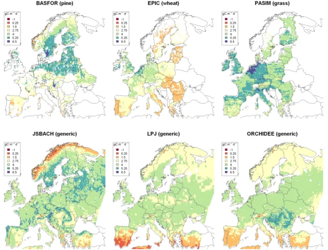
All models are run using the same climatic input and the same 0.25 × 0.25◦spatial resolution. Only the generic mod-els are applied to all grid cells (Table 1). Each model uses soil data from the Harmonized World Soil Database (HWSD v 1.2; FAO et al., 2012) unless indicated otherwise in the following model descriptions. Simulation results do not in-clude the impact of fire, pests and diseases. An example of each model’s output, average NPP in 1971–2000, is shown in Fig. 2.
2.3.1 BASFOR (Scots pine)
BASFOR (Van Oijen et al., 2005) is a forest model that runs with a daily time step and requires as environmental in-puts: weather, nitrogen deposition, CO2 concentration, soil
carbon and nitrogen content, and soil water retention char-acteristics. For the present risk analysis, we use the model
as parameterized for Scots pine based on forest inventory data from four different European countries (Van Oijen et al., 2013a). Information on soils and on atmospheric nitro-gen deposition is based on work by Cameron et al. (2013). The model is run with a fixed forest rotation length of 80 years with regularly spaced thinnings, for eight age-cohorts (Cameron et al., 2013). Trees respond to drought by reducing carbon uptake, accelerating senescence and changing alloca-tion in favour of the roots, but mortality is not simulated. The model has been used for the analysis of carbon and nitro-gen fluxes in Norway spruce forest (Van Oijen et al., 2011) and for assessing the impact of climate change on carbon se-questration in forests in the United Kingdom (Van Oijen and Thomson, 2010).
2.3.2 EPIC (winter wheat)
EPIC (Environmental Policy Integrated Climate; Williams et al., 1989) is an agro-ecosystem model running with a daily time step. It simulates crop development and yield, hydro-logical, nutrient and carbon cycles and a wide range of crop management activities. Required input data include mini-mum and maximini-mum temperature (◦C), precipitation (mm), global radiation (MJ m−2), CO2concentration, soil
proper-ties (bulk density (g cm−3), base saturation (%), percentages of soil organic carbon, sand, silt and clay), crop heat re-quirement and crop management (planting dates, tillage op-erations, fertilizer application). In the present study, winter wheat is simulated in 1 year mono-crop rotations on all the available European cropland. It is simulated as a winter crop, with varieties based on growing season length and heat re-quirements distinguished for Atlantic, alpine, boreal, con-tinental and Mediterranean climatic zones. The simulations are performed with current fertilizer input levels. A detailed description and evaluation of this implementation is provided by Balkoviˇc et al. (2013).
Plant growth is simulated using the concept of radiation-use efficiency (Monteith, 1977). Potential biomass increase is calculated as a function of photosynthetically active radia-tion and leaf area index. CO2fertilization increases
radiation-use efficiency and stomatal resistance, thereby reducing tran-spiration (Stockle et al., 1992). Crop yield is calculated via a harvest index, determining yield as a fraction of above-ground biomass. Daily heat unit accumulation determines leaf area growth and senescence, canopy height, nutrient up-take, harvest index and date of harvest. Temperature also determines potential ET, which is calculated with the Har-greaves method. Actual ET is governed by leaf area index and the water content and depth of the root zone. Both ac-tual ET and biomass increase are reduced when the plant-available soil water level is less than 25 % of the maximum. Heterotrophic respiration is also temperature and moisture dependent following the carbon and nitrogen cycle model of Izaurralde et al. (2006).
Previously we have evaluated and used the EPIC model for hindcasting assessments of the impact of extreme dry and wet weather on crop production (Van der Velde et al., 2010, 2012).
2.3.3 PASIM (grassland)
PASIM, the Pasture Simulation model (Riedo et al., 1998; Vuichard et al., 2007) is a multi-year biogeochemical model that simulates water, carbon and nitrogen cycles in grassland systems at the plot scale on a daily to sub-daily time step. Soil processes are based on the CENTURY model of Par-ton et al. (1988). Photosynthetically assimilated carbon is ei-ther respired or allocated dynamically to one root compart-ment and three shoot compartcompart-ments. Accumulated above-ground biomass is removed by either cutting or grazing, or enters a litter pool. Soil organic carbon (SOC) is represented in three pools (active, slow and passive) with different po-tential decomposition rates, while above and below-ground plant residues and organic excreta are partitioned into struc-tural and metabolic pools. The nitrogen cycle considers three types of nitrogen inputs to the soil via atmospheric nitrogen deposition, fertilizer nitrogen addition, and symbiotic nitro-gen fixation by legumes. The inorganic soil nitronitro-gen is avail-able for root uptake and may be lost through leaching, am-monia volatilization and nitrification/denitrification, the lat-ter processes leading to nitrous oxide (N2O) gas emissions
to the atmosphere. Management includes nitrogen fertiliza-tion, mowing and grazing and can either be set by the user or optimized by the model (Vuichard et al., 2007; Graux et al., 2011). In this model version, nitrogen fixation is simu-lated by assuming a constant legume fraction, an algebraic method for SOC equilibrium search (Lardy et al., 2011) is used to reduce computation time, and grassland nitrogen fer-tilization corresponds to current farming practices (Weiss and Leip, 2012). Stomatal conductance depends on soil water content and atmospheric vapour pressure and CO2
concentra-tion. Drought-induced stomatal closure leads to a decreased photosynthetic rate and increases in vegetation temperature as well as autotrophic and heterotrophic respiration.
2.3.4 JSBACH (generic vegetation)
The land surface scheme JSBACH (Raddatz et al., 2007) simulates land–atmosphere exchanges of energy, water and carbon at 30 min temporal resolution. The representation of canopy processes is based on the BETHY model which cou-ples energy and water balance with photosynthesis through stomatal conductance (Knorr, 2000) to which a module for phenology and a simple carbon cycle scheme including sev-eral pools for vegetation, litter and soil carbon have been added (Raddatz et al., 2007). Canopy conductance is addi-tionally constrained by soil water availability (Raddatz et al., 2007). In the version used for this study, soil hydrology is represented by a five layer scheme (Hagemann, 2014). The
Figure 2. Average net primary productivity (NPP, g C m−2d−1)for April to September in 1971–2000 for six different vegetation models.
fractional coverage of land by several plant functional types is prescribed based on GLC2000 (Bartholomé and Belward, 2005) and MODIS VCF land cover information (Hansen et al., 2003). Disturbances are not explicitly simulated but taken into account by the mean residence time of carbon pools (Raddatz et al., 2007).
2.3.5 LPJmL (generic vegetation)
LPJmL (Sitch et al., 2003; Bondeau et al., 2007; Gerten et al., 2004) is a dynamic global vegetation model that simu-lates process-based terrestrial vegetation dynamics and phys-iology and land–atmosphere carbon and water fluxes. Its capability to adequately represent ecosystem responses to changing precipitation has been demonstrated by Gerten et al. (2008). Vegetation is represented as 10 plant functional types (PFTs) which differ in their bioclimatic limits and mor-phological, phenological and physiological parameters. Bio-climatic limits determine the ability of a species to establish under a given climate, ecophysiological parameters deter-mine the ability to survive and to become dominant species. Each plant functional type is represented by an average indi-vidual covering a fraction of the grid cell. For each average
individual of the 10 PFTs, LPJmL simulates photosynthe-sis and respiration, the allocation of accumulated carbon to the plant’s compartments (leaves, stem, roots, reproductive organs). Vegetation structure and dynamics are updated on an annual time step, while photosynthesis, evapotranspira-tion and soil water exchange are calculated daily. The soil consists of two layers with water content driven by precipi-tation, snowmelt, percolation, runoff and evapotranspiration. PFTs differ in their fraction of roots in the upper and lower soil layer representing shallow- and deep-rooting plants.
Evapotranspiration is calculated for each PFT as a function of soil moisture supply and atmospheric demand. If atmo-spheric demand is higher than water supply, canopy conduc-tance is reduced until transpiration equals the supply. This di-rectly influences photosynthesis rates by reduced diffusion of CO2into the leaf intercellular space. Canopy photosynthesis
and thus gross primary productivity are calculated for each PFT based on a modified Farquhar photosynthesis model (Farquhar et al., 1980; Collatz et al., 1991) driven by ab-sorbed photosynthetically active radiation, temperature and leaf intercellular CO2concentration under the assumption of
optimal nitrogen availability. Net primary productivity (NPP) is the difference between gross primary productivity GPP
and carbon lost from growth and maintenance respiration. Net ecosystem productivity is derived from the difference of NPP and heterotrophic respiration (Rh). Heterotrophic res-piration results from the decomposition of litter and soil or-ganic matter and is temperature and moisture dependent (for details see Sitch et al., 2003).
2.3.6 ORCHIDEE (generic vegetation)
ORCHIDEE (Krinner et al., 2005) is a land surface model that simulates carbon, water and energy exchanges within ecosystems, and between the land and the atmosphere. The land vegetation is represented by 12 plant functional types (PFTs). The definition of a PFT accounts for physiognomy (tree or grass), leaf types (needle-leaf or broad-leaf), phenol-ogy (evergreen, summer-green or rain-green), the photosyn-thetic pathway for crops and grasses (C3 and C4)and the
climatic regions (boreal, temperate and tropical). Exchanges of energy and water are calculated following Ducoudré et al. (1993) and de Rosnay and Polcher (1998) at 30 min time steps.
Potential transpiration is limited by aerodynamic resis-tance above and within the canopy and stomatal resisresis-tance (Ducoudré et al., 1993), and potential evaporation is propor-tional to the humidity difference between air and air at satu-ration for soil temperature. Bare soil evaposatu-ration is the max-imum upward hydrological flux permitted by diffusion if this flux is smaller than potential evaporation (d’Orgeval et al., 2008). When root zone soil moisture falls below 40 %, stom-atal conductance, photosynthesis and evapotranspiration de-crease linearly, reaching zero for entirely dry soils (McMur-trie et al., 1990). Atmospheric dryness also affects these pro-cesses, following Ball et al. (1987). The 11 layer scheme for the upper 2 m of soil is based on the CWRR model (Bruen, 1997). Layers are thinner near the surface (De Rosnay et al., 2002). Vertical water flow is based on the one-dimensional Darcy equation (De Rosnay et al., 2002). The bottom bound-ary condition is set to be free drainage.
GPP is calculated every 30 min using the Farquhar et al. (1980) and Collatz et al. (1992) leaf scale equations for C3
and C4PFTs respectively. Net primary productivity (NPP),
plant growth, maintenance respiration, mortality, litter and soil organic matter decomposition are calculated on a daily time step following GPP. Water stress alters carbon alloca-tion and accelerates leaf senescence (Krinner et al., 2005). The model accounts for fires but not for vegetation dynamics. Drought has lagged effects on leaf area index (LAI) through reduced production of carbon reserves for the following year, but does not directly increase tree mortality. Heterotrophic respiration (Rh) is coupled positively to NPP on time scales of weeks to months via the short-lived litter and labile soil carbon pools. Decomposition increases with warmer temper-atures, according to a Q10law, and with relative soil moisture
(Krinner et al., 2005).
2.4 Normalized Difference Vegetation Index (NDVI)
The Normalized Difference Vegetation Index (NDVI, Tucker, 1979) is a radiometric measure of vegeta-tion photosynthetic capacity. It compares the reflectance difference between photosynthetically active radiation (PAR, ∼ 400–700 nm) and near-infrared radiation (NIR, ∼700–1100 nm). The index is indicative of the abundance of chlorophyll content in the vegetation canopy (Myneni et al., 1992), and is highly correlated with gross primary produc-tivity (Veroustraete et al., 1996). The index is derived from satellite observations, made globally over long time periods. It is used in the present study for two purposes: to determine the timing of the growing season at different latitudes in Eu-rope and to provide independent data for testing the perfor-mance of the six models including the PRA.
We use the latest version of the Global Inventory Modeling and Mapping Studies (GIMMS) NDVI data set (NDVI3g) generated from the Advanced Very High Resolution Ra-diometer (AVHRR). The AVHRR instruments aboard a series of NOAA polar-orbiting meteorological satellites (NOAA 7, 9, 11, 14, 16–19) have observations in multiple spectral bands from 1981 to the present. As the first set of instruments that have non-overlapping spectral bands from visible (VIS) and near-infrared (NIR) ranges, NDVI can be calculated as (NIR−VIS) / (NIR+VIS). The GIMMS data set has been recalibrated recently to improve data quality at northern high latitudes, and an overall uncertainty of ±0.005 NDVI units is achieved independent of time frame (Pinzon and Tucker, 2014). It has also been corrected for calibration, viewing geometry, volcanic aerosols, and other effects not re-lated to vegetation change (Pinzon and Tucker, 2014; Pinzon et al., 2005; Tucker et al., 2005).
The GIMMS NDVI3g data set contains NDVI values from 1981 to 2012 with 15 day temporal and 8 km spatial resolu-tion, of which the years 1982–2010 are used in the present study. The data set has been used to explain diminishing veg-etation seasonality in the northern high latitudes over the past 30 years (Xu et al., 2013), vegetation greening and brown-ing trends (De Jong et al., 2013), latitudinally asymmetric vegetation growth trends with small increases in the South-ern Hemisphere and larger increases at high latitudes in the Northern Hemisphere (Mao et al., 2013), global trends of seasonality change in natural areas (Eastman et al., 2013) and an earlier start of the growing season in Fennoscandia (Høgda et al., 2013).
Figure 3a shows a map of the average value of the NDVI across Europe in the years 1982–2010, months April–September. The lowest NDVI values are in the cold north and the dry Mediterranean. The same map further shows the division in three latitudinal bands (“North”, “Mid”, “South”) that we use for summarizing results later in the study. The unbroken lines in Fig. 3b show the intra-annual progression of NDVI averaged over the years per lat-itudinal band. Seasonal peak NDVI is reached by May in the
Figure 3. NDVI in Europe: (a) average values of NDVI for April to September in 1982–2010. (b) Continuous lines: average monthly values
of NDVI in the latitudinal bands delineated in (a); the thin dashed lines are for the years 2001, 2002, 2004 and 2005, the bold dashed line is for 2003.
south, a month later at mid-latitude and yet another month later in the north. Based on these observations, we used a common time interval of April to September for the calcu-lation of the SPEI at all latitudes. This period is close to the period of April–August in which different kinds of extreme events, but predominantly water scarcity, were shown to re-duce gross primary productivity in Europe the most in the years 1982–2011 (Zscheischler et al., 2014, their Fig. 8). To indicate inter-annual variation, the five dashed lines in Fig. 3b represent the individual years 2001, 2002, 2004 and 2005, with 2003 in bold. The variation between years is much lower than between months, even when, as here, an extreme year like 2003 is included.
2.5 Probabilistic Risk Analysis (PRA) 2.5.1 Theory for PRA
Following the procedure outlined in greater detail by Van Oi-jen et al. (2013b), we distinguish environmental and system variables, denoted as env and sys. Sys variables are expected to be sub-optimal when env variables reach levels that con-stitute hazardous conditions. Numerically, risk (R) is defined as the expectation of system loss, i.e. the amount by which average system performance is less than it would be under continuously non-hazardous conditions:
R = E(sys|env non-hazardous) − E(sys), (1)
where E(sys) is the overall expectation value of the sys vari-able, and E(sys|env non-hazardous) is the expectation value of the sys variable when conditions are not hazardous. The probability of env variables assuming hazardous values is de-noted as P (hazardous), or P (H ) in short. Vulnerability (V )
has, in contrast to most previous applications of risk analysis, a precise quantitative definition:
V = E(sys|env non-hazardous) − E(sys|env hazardous), (2)
with the obvious interpretation of terms. This definition of vulnerability as the difference in sys performance between non-hazardous (“good”) and hazardous (“bad”) conditions allows us to write R alternatively as:
R = P (H ) · V . (3)
Equations (1) and (3) are mathematically equivalent, giving the same estimates of risk. The last equation shows that the risk to sys variables can be decomposed into two terms: the probability of hazardous environmental conditions and the vulnerability of the system.
2.5.2 Application of PRA in this study
The env variable in the present study is the SPEI, and haz-ardous conditions are mostly defined as SPEI being less than −1 (Sect. 2.2). We carry out the PRA for five different sys variables: net primary productivity (NPP), heterotrophic res-piration (Rh), net ecosystem productivity (NEP), soil water content (SWC) and evapotranspiration (ET). Values for the sys variables are generated by the six different vegetation models. PRAs are carried out for each grid cell separately, and for two time periods: 1971–2000 and 2071–2100. P (H ) is calculated as the fraction of the thirty years in each pe-riod with SPEI lower than the threshold. Likewise, the var-ious expectation values E(sys|env) are calculated from the frequency distribution of sys values over the thirty years.
The main outcomes of the PRA are vulnerabili-ties and risks, typically expressed in absolute values
(e.g. g C m−2d−1for the carbon fluxes). In the last two
fig-ures of the paper, we express them as fractions of system performance in non-hazardous years.
An additional PRA is carried out using NDVI as the sys variable. Drought vulnerability and risk for NDVI are not of interest themselves, but comparison of V and R for NDVI with those for model outputs provides a coarse empirical check of the accuracy of the model-based analysis.
2.5.3 Sensitivity analysis of the PRA
After the main PRAs outlined above, we subject NPP out-put from one of the generic models, LPJmL, to additional PRAs to assess the robustness of our results. First, we as-sess how vulnerability and risk estimates change when a dif-ferent SPEI threshold is chosen to demarcate hazardous and non-hazardous conditions. We vary the SPEI threshold over the sequence −2, −1.5, −1, −0.5, 0. We then test the idea that a lag time in the response of sys to env should be ac-counted for. The half-yearly periods for calculating NPP are kept at April–September, but the half-yearly SPEI periods are shifted to be one, two or three months earlier. In a third and final sensitivity analysis, we vary the climate scenario by reducing inter-annual weather variability, while conserv-ing 30 year long-term averages of annual and seasonal values (see Sect. 2.1).
3 Results
3.1 The basic PRAs
Each of the six models has been used to calculate PRAs for each grid cell (the number of which varied between models, Table 1). Per grid cell, ten PRAs have been carried out by each model to assess five variables (NPP, Rh, NEP, SWC, ET) in two time periods (1971–2000, 2071–2100). These PRAs represent the core results of this study.
To clarify the approach, we show in Fig. 4 all the details of one example: the PRA for NPP in 1971–2000 according to model LPJmL. The different steps in the PRA are repre-sented by the different panels of the figure. Panel A shows the average NPP in the non-hazardous years, i.e. the years with SPEI for months 4–9 above −1. Panel B shows the same for the hazardous years. Vulnerability, shown in the next panel, is calculated as the difference between the two: C = A–B. The frequency of years with SPEI below −1, i.e. the proba-bility of hazardous conditions, P (H ), is depicted in panel D. Finally, risk, shown in the last panel, is the product of vulner-ability and P (H ), so E = C × D. In this example, vulnerabil-ity is largest in the south, but P (H ) varies little across Eu-rope. According to this particular vegetation model, the risk to NPP posed by drought (SPEI < −1) is therefore highest in the Mediterranean because the vegetation is more vulnera-ble to exceptional droughts there than elsewhere, and not be-cause of a higher drought frequency. But note that SPEI < −1
represents far drier conditions in the Mediterranean than fur-ther north.
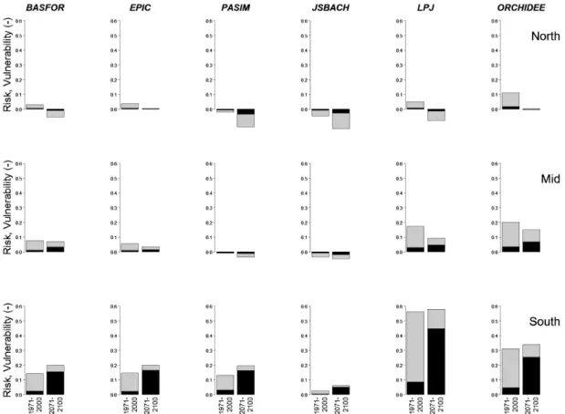
Figure 5 summarizes the risk analyses for NPP per latitu-dinal band for all six models, and for both time periods. The bars show relative vulnerability, i.e. vulnerability divided by the NPP at the same location under contemporaneous non-hazardous conditions. The black part of each bar is the risk, also in relative terms. The ratio of the black part and the whole bar, i.e. risk divided by vulnerability, is equal to the hazard probability, P (H ) (Eq. 3). Most models indicate that relative vulnerabilities and risks increase from north to south, in both time periods. Note that in some cases, mainly found in the north, the values are negative. These are conditions where dry years (SPEI < −1) are in fact the more favourable for NPP, likely because of climatic variables that co-vary with SPEI. During dry years in the period 1971–2000, ra-diation in the north was on average reduced by only 0.1 %, which is unlikely to be of any significance, but temperature was 0.2◦C higher, possibly extending growing seasons and stimulating NPP.
Overall the relative risks to NPP are higher in 2071–2100 than in the earlier period, especially in the south according to all six models. The main reason is an increase in hazard probability rather than an increase in vulnerability.
The three ecosystem models show very similar results, especially in the most sensitive region, the south. This is despite the models simulating different vegetation types and partly different sets of grid cells. In contrast, the three generic models differ strongly from each other, with vulnerabilities and risks to NPP decreasing in the order LPJmL > ORCHIDEE > JSBACH.
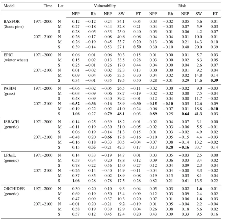
The results of the PRAs for all five model output variables and both time periods are summarized in Table 2. Note that the values in the table are in absolute units, in contrast to Fig. 5. The highest and lowest values of vulnerability and risk, across all models, are indicated for each variable in bold italic typeface.
The vulnerabilities and risks for Rh differ strongly be-tween models. In over half the cases, the ecosystem mod-els show negative vulnerability and risk for Rh (i.e. drought increases soil respiration). The vulnerabilities found by the generic models are always positive (i.e. drought reduces res-piration), likely because in those models, Rh anomalies are tightly coupled with NPP trough fast carbon pools. NEP can be calculated as NPP minus Rh, and likewise NEP vulner-ability and risk can be calculated from those for NPP and Rh. Therefore the results for NEP vary strongly between the models as well, with vulnerabilities that are always less than for NPP in the case of the generic models, but often the op-posite for the ecosystem models.
The vulnerability and risk for SWC also vary consider-ably among the models, with lowest values estimated by the two generic models that have low average SWC (Table 1): LPJmL and ORCHIDEE. But all models agree that SWC vul-nerabilities do not differ much between latitudinal bands or
Figure 4. Probabilistic risk analysis (PRA) for net primary productivity (NPP, g C m−2d−1)in 1971–2000 using model LPJmL. The con-sidered hazard is drought, defined as SPEI < −1. All values are for the months April–September: (a) NPP in non-hazardous years; (b) NPP in hazardous years; (c) vulnerability of NPP (= A–B); (d) probability of hazard; and (e) risk to NPP (= C × D).
time periods. Climate change does induce a spatial gradient to the risk, with highest values in the south. Vulnerability and risk for ET show greater spread among the ecosystem models (with PASIM simulating relatively low values in both time periods) than among the generic models. Climate change in-creases risks mainly in the south.
3.2 Sensitivity analysis of the PRA
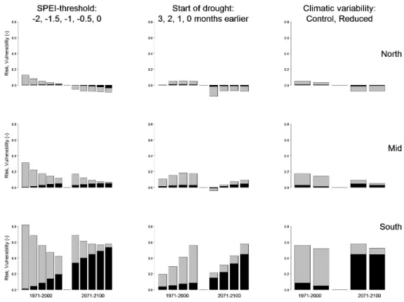
Results of the assessment of the robustness of the PRA to various assumptions are shown in Fig. 6. The figure shows relative values of vulnerability and risk for NPP as simu-lated by model LPJmL for both time periods. The left column shows how results depend on the choice of the environmen-tal threshold, which is varied from −2 to 0 by half-unit steps. The bars in the middle are for the default SPEI threshold of −1, thus showing the same results as in Fig. 5. When the threshold is increased, a greater fraction of years is classified as hazardous, so risk increases relative to vulnerability. Vul-nerability itself decreases, mainly in the first time period. In the second time period, vulnerability is nearly independent of the choice of the threshold.
In the second sensitivity analysis, shown in the middle col-umn of Fig. 6, the timing of the half-year long SPEI pe-riod has been shifted by different amounts: 0, −1, −2, −3
months. So in this case the rightmost bars, with shift equal to zero months, repeat the results of Fig. 5. Overall, vulnera-bility and risk are highest for the zero shift, i.e. drought peri-ods that cover the same six months (April–September) as are chosen for NPP.
In the final sensitivity analysis, shown in the right column, the models have been run with two climate scenarios: the control scenario used in all other assessments, and the re-duced variability scenario (Sect. 2.1). The results are very robust against this change, for both time periods.
3.3 Comparisons with NDVI
To test the performance of the models, we examine how the spatial patterns over Europe simulated by the models corre-late with the spatial pattern of NDVI observations. Table 3 shows the correlations across all grid cells of model outputs with NDVI. With the single exception of evapotranspiration as simulated by PASIM, the correlations are positive, and strongly so for the fluxes simulated by the generic models (r > 0.6).
A second test is aimed at evaluating not the original model outputs but the vulnerabilities and risks derived from them. To this end, we have applied the risk analysis to NDVI and report in Table 4 the correlations between V and R for NDVI
Table 2. Drought vulnerability and risk of the carbon and water balance across Europe. Averages for two time periods and three
latitudi-nal bands, calculated by six models. N is above 55◦N, M is between 45 and 55◦N, S is below 45◦N. NPP is net primary productivity (g C m−2d−1), Rh is heterotrophic respiration (g C m−2d−1), NEP is net ecosystem productivity (g C m−2d−1), SW is soil water content (mm), ET is evapotranspiration (mm d−1). A bold font is used for the most extreme vulnerabilities and risks for each variable.
Model Time Lat Vulnerability Risk
NPP Rh NEP SW ET NPP Rh NEP SW ET BASFOR 1971–2000 N 0.12 −0.12 0.24 34.1 0.05 0.03 −0.02 0.05 5.6 0.01 (Scots pine) M 0.27 −0.18 0.44 32.8 0.21 0.04 −0.03 0.07 5.9 0.03 S 0.28 −0.05 0.33 25.0 0.40 0.05 −0.01 0.06 4.2 0.07 2071–2100 N −0.26 −0.17 −0.08 40.6 −0.06 −0.04 −0.04 −0.01 10.0 −0.01 M 0.26 −0.19 0.45 33.7 0.20 0.13 −0.08 0.21 14.3 0.10 S 0.39 −0.14 0.53 27.1 0.50 0.30 −0.10 0.40 20.0 0.39 EPIC 1971–2000 N 0.06 0.01 0.06 30.3 0.15 0.01 0.00 0.01 5.7 0.03 (winter wheat) M 0.15 0.02 0.13 33.5 0.28 0.03 0.00 0.02 6.3 0.05 S 0.25 −0.01 0.26 17.0 0.44 0.04 0.00 0.04 2.6 0.07 2071–2100 N 0.01 −0.02 0.02 32.3 0.13 0.00 0.00 0.01 9.2 0.04 M 0.09 0.04 0.05 33.5 0.30 0.04 0.02 0.02 14.8 0.14 S 0.34 −0.01 0.35 19.5 0.50 0.28 −0.01 0.29 14.6 0.39 PASIM 1971–2000 N −0.06 −0.02 −0.05 26.5 −0.11 −0.02 0.00 −0.02 9.0 −0.03 (grass) M −0.03 −0.09 0.06 38.7 −0.19 −0.02 −0.02 0.00 7.5 −0.04 S 0.48 0.09 0.40 39.2 −0.01 0.12 0.04 0.08 11.7 −0.02 2071–2100 N −0.52 −0.36 −0.16 28.9 −0.30 −0.15 −0.10 −0.05 12.6 −0.09 M −0.19 −0.22 0.02 41.0 −0.24 −0.06 −0.07 0.01 18.8 −0.10 S 1.06 0.27 0.79 48.1 −0.03 0.89 0.25 0.64 41.3 −0.03 JSBACH 1971–2000 N −0.14 0.25 −0.39 18.2 −0.01 −0.02 0.04 −0.07 3.1 0.00 (generic) M −0.11 0.19 −0.30 31.0 −0.05 −0.02 0.03 −0.06 5.5 −0.01 S 0.06 0.19 −0.14 31.3 0.15 0.01 0.03 −0.02 4.9 0.02 2071–2100 N −0.48 0.20 −0.66 17.8 −0.16 −0.10 0.05 −0.15 4.4 −0.03 M −0.16 0.18 −0.33 30.5 −0.04 −0.07 0.08 −0.14 13.2 −0.02 S 0.15 0.35 −0.21 42.3 0.17 0.13 0.28 −0.16 33.7 0.14 LPJmL 1971–2000 N 0.14 0.33 −0.19 14.7 0.01 0.03 0.05 −0.03 2.5 0.00 (generic) M 0.53 0.34 0.20 18.8 0.12 0.09 0.06 0.03 3.4 0.02 S 0.78 0.22 0.56 15.0 0.27 0.12 0.04 0.09 2.3 0.04 2071–2100 N −0.26 0.14 −0.40 14.9 −0.11 −0.04 0.04 −0.08 3.3 −0.02 M 0.37 0.35 0.02 18.9 0.08 0.19 0.15 0.03 8.1 0.04 S 1.06 0.28 0.78 17.5 0.28 0.82 0.21 0.61 13.5 0.22 ORCHIDEE 1971–2000 N 0.30 0.20 0.10 9.3 −0.04 0.05 0.03 0.02 1.6 −0.01 (generic) M 0.69 0.19 0.50 13.4 0.09 0.12 0.03 0.09 2.4 0.02 S 0.47 0.09 0.37 10.3 0.20 0.07 0.01 0.06 1.6 0.03 2071–2100 N −0.01 0.20 −0.21 9.2 −0.19 0.01 0.05 −0.04 2.2 −0.04 M 0.58 0.19 0.39 12.9 0.04 0.26 0.08 0.18 5.6 0.02 S 0.57 0.12 0.45 12.4 0.20 0.43 0.09 0.33 9.5 0.16
with those for NPP and ET. We have restricted this test to NPP and ET because changes in NDVI reflect changes in leaf area which has direct effects only on the fluxes of car-bon and water through the plants. With the exception of ET risk calculated by PASIM, all correlations are again positive, but generally less strong than for the original sys variables (Table 4).
4 Discussion
4.1 Theory and current application of probabilistic risk analysis
The method of PRA that we have applied here was proposed in a recent publication (Van Oijen et al., 2013b). We argued there that the strengths of the method included its quanti-tative nature, its simplicity, the possibility of choosing any env variables and sys variables of interest, as well as the
Figure 5. Drought risk analysis for NPP in two time periods (1971–2000, 2071–2100), for the six different models. Top row: above 55◦N; mid row: between 45 and 55◦N; bottom row: below 45◦N (see Fig. 3a). The whole bars depict vulnerability (V ), the black parts are risks
(R). V and R are expressed in relative terms, as fractions of NPP under non-hazardous conditions. Drought probabilities, P (H ), are equal to R/V .
Table 3. Correlations of NDVI with model outputs at the
Euro-pean scale (where n is model-specific, see Table 1). NDVI and out-puts are averages for April–September over multiple years (NDVI: 1982–2010, outputs: 1971–2000). Variables as in Table 2.
MODEL NPP Rh NEP SWC ET
BASFOR (Scots pine) 0.36 0.21 0.46 0.02 0.68 EPIC (winter wheat) 0.20 0.22 0.17 0.52 0.62 PASIM (grass) 0.39 0.20 0.52 0.07 −0.32 JSBACH (generic) 0.79 0.76 0.79 0.18 0.70 LPJmL (generic) 0.79 0.75 0.65 0.54 0.67 ORCHIDEE (generic) 0.76 0.74 0.61 0.33 0.66
applicability to any environmental thresholds and any time lag between env and sys. These strengths seem to be borne out by the comprehensive application of the method in the present study. The main advantage of the method may be that it allows decomposition of risk into two multiplicative terms: the probability of hazardous conditions and the vulnerability of the system.
Our analysis focused on the half-year period of April to September, which was estimated from NDVI observations
Table 4. Correlations of vulnerabilities and risks calculated for
NDVI with those calculated for model outputs of NPP and of ET at the European scale (where n is model-specific, see Table 1). All val-ues are averages for April–September over multiple years (NDVI: 1982–2010, outputs: 1971–2000).
MODEL Vuln(NPP) Risk(NPP) Vuln(ET) Risk(ET) BASFOR (Scots pine) 0.24 0.25 0.29 0.29 EPIC (winter wheat) 0.10 0.11 0.20 0.22 PASIM (grass) 0.22 0.20 0.01 −0.04 JSBACH (generic) 0.20 0.19 0.18 0.21 LPJmL (generic) 0.41 0.42 0.40 0.41 ORCHIDEE (generic) 0.38 0.40 0.47 0.48
(Fig. 3b) as the main period of high carbon uptake and water use by vegetation in the different European climatic zones. Climate change toward drier summers may affect the an-nual pattern of vegetation activity, but shifts to early spring or late autumn will be constrained by the lower levels of solar radiation. The risk analysis could be refined by using slightly different time periods for different parts of Europe, more closely matching the growing season at each location. NDVI is a convenient proxy for identifying this period for large regions, given its global availability and high spatial
resolution. Moreover, the high spatiotemporal coverage of NDVI allowed us to test our models and risk analyses in var-ious ways as shown in Tables 3 and 4, and discussed below. In contrast to NDVI, use of the comparatively sparse set of European eddy covariance towers, which also have footprints considerably smaller than the areas of grid cells, would not have afforded the same capability.
Because we focused on half-year periods, temporary in-terruptions of ecosystem activity by droughts of shorter du-ration are not included in our analyses, especially if vege-tation in models recovered quickly after the drought ended. But such short-term droughts would then not play a signifi-cant role in the long-term carbon balance of the vegetation. Similarly, use of longer periods than the growing season, e.g. whole years, would have caused dilution of the drought signal by precipitation in the off-season.
The quality of our ecosystem vulnerability assessment, in particular for future conditions, is limited by how well the six different models represent processes of adaptation to en-vironmental change. The models simulate vegetation change (migration, fire disturbance in some models, acclimatization and physiological adaptation) only to a limited degree. Three of the six models are dynamic vegetation models which al-low for replacement of plant functional types by others when the environment changes, but migration is not explicitly sim-ulated. However, in Europe, land use change, forest man-agement and landscape fragmentation are likely to limit fu-ture ecosystem migration, except in the very few regions where ecosystems are not managed. Physiological adapta-tion is simulated to some extent by the models (e.g. stomatal closure with increased atmospheric CO2 concentration and
drought, increased allocation to roots when soil resources become limiting, temperature optimum of photosynthesis). It is conceivable that the vegetation types will adapt more strongly to the new climatic conditions than can be foreseen at this stage. However, our main results seem to be robust be-cause additional adaptation processes would be likely to re-duce vulnerability, whereas our risk decomposition already identified increased hazard probability as the greater threat (Sect. 3.1). Also, changes in vulnerability would have to be extreme and much more favourable in the Mediterranean area than elsewhere to overturn our further prediction that the southern part of Europe is at the greatest risk. Regarding the drought hazard itself, a consistent drying trend in Southern Europe, with increased drought extremes, is also predicted in the recent work of Jacob et al. (2014).
4.2 Vulnerabilities and risks in the years 1971–2000
We found that relative drought vulnerability of NPP in the early period, 1971–2000, was highest in the south (Fig. 5). This result seems fairly robust as it was found by all six models. Numerically there was variation, with LPJmL esti-mating higher vulnerabilities than the other models, and JS-BACH lower ones. The exceptional vulnerabilities of these
two generic models can partly be explained by their widely differing estimates of the average amount of water in the root zone (SWC) of the vegetation (Table 1), but SWC var-ied strongly for the other models, too. NPP is the difference between GPP and autotrophic respiration, and high drought sensitivity of GPP as simulated by LPJmL was already re-ported by Zscheischler et al. (2014).
Despite the relatively high NPP vulnerabilities in the south, the risks were commonly estimated as being low (< 10 %) due to the low probability of drought. The very similar responses of the three ecosystem models (vulnera-bility < 15 %, risk < 5 %) were not expected, given that the models simulate very different ecosystem types, and model structures are very different. This may be the result of com-pensating factors. Wheat and grass are more shallow-rooting than trees, making them more drought sensitive in the short term, but they can more easily be irrigated or re-sown and suffer less from carry-over effects in the case of consecutive drought years.
Unlike for NPP, vulnerability of Rh did not show a con-sistent latitudinal trend for most of the models (Table 2). For all latitudes, the ecosystem models estimated lower Rh vul-nerabilities than the generic models did. In fact, many esti-mates by the ecosystem models were negative, indicating that the droughts increased soil respiration. It is likely that this is the consequence of differences between the models in stress response functions, with soil organic matter turnover be-ing mainly regulated by temperature in the ecosystem els, and mainly by water availability in the generic mod-els. The systematic disagreement between the two model types is surprising, and it points to significant uncertainty about the regulation of organic matter turnover. However, de-spite model differences, risks for Rh were always assessed as small (< 0.35 g C m−2d−1)because of low P (H ).
The estimates for drought vulnerability and risk to NEP were generally highest in the south, but the values varied considerably among models. The drought response of NEP tended to follow that of NPP more closely than that of Rh for most models except JSBACH. JSBACH simulated much greater drought-induced reductions of Rh than of NPP and was therefore the only model to predict increases of NEP under drought even in the south and in both time periods. To quantify the degree to which the vulnerability of NEP was generally more closely related to NPP vulnerability than to Rh vulnerability, we carried out a correlation analysis for each model. The vulnerability correlation coefficients for NEP–NPP ranged from 0.70 to 0.96 across all models, whereas the NEP–Rh correlation coefficients were in the range −0.65 to 0.11. The results for risk were similar, con-firming that drought effects on NPP were stronger determi-nants of changes in net carbon flux than drought effects on Rh.
The models seemed more consistent in their estimates of vulnerability and risk for SWC and ET, but as these variables were mainly quantified to help understand the underlying
risk for each of the five examined sys variables. Invariably, the highest values were found in the period 2071–2100. For carbon fluxes this result can partly be explained by CO2
sen-sitivity: with a general increase in carbon fluxes because of elevated CO2, differences between wet and dry conditions
may be expected to increase as well. Averaged across the models, the increases in NPP, Rh and NEP were 17, 22 and 10 %, respectively. However, vulnerabilities generally in-creased less than that, and even dein-creased slightly in mid-Europe and the north, possibly because of elevated CO2
in-creasing drought tolerance by inducing stomatal closure. In contrast, climate change is expected to increase risks strongly, particularly in the south, according to the sce-nario and models used in this study. The underlying cause is mainly the probability of drought, which increases far more than vulnerabilities do. Risks exceeding 0.25 g C m−2d−1 are predicted for carbon sequestration (NEP) in the south by most models, amounting to reductions in carbon sequestra-tion of 20 to 80 %. In contrast, the model JSBACH shows different results, even predicting negative risk for NEP at all latitudes. JSBACH differs from the other models in that it predicts a far greater drought vulnerability of Rh than of NPP. Because the model predicts that carbon uptake is re-duced less than carbon loss under future droughts, it thus pre-dicts increased carbon sequestration in drought years. This is a counter-intuitive result, which needs to be evaluated more closely in future work.
The southward increasing risks to carbon fluxes that are predicted by all models except JSBACH, are mirrored by in-creasing risks to SWC and ET. In relative terms (compare Table 2 with the European average values given in Table 1), risks to SWC and ET tend to vary to a similar degree, sug-gesting that the risk to water use by vegetation is controlled by soil water availability rather than by stomatal regulation or atmospheric feedbacks.
4.4 Comparison of model results with NDVI
All of the models have been used in different applications, and their predictions have been compared to observations (see Sect. 2). However, this study is the first where the mod-els have been used in PRA, except for a preliminary applica-tion using forest model BASFOR (Van Oijen et al., 2013b). Testing a probabilistic risk analysis is difficult: to test
prob-five model outputs (Table 3). Because these calculations are at the European scale, we should in fact expect reasonably strong positive correlations, reflecting the contrast between productive vegetation in central Europe versus the low LAI and vegetation activity in the dry Mediterranean area and the cold far north. This is borne out by the data in Table 3 which show generally high correlations for the four fluxes, with as sole exception the negative correlation of NDVI with ET predicted by PASIM. The relatively low correlations for the grassland and crop ecosystem models PASIM and EPIC are explained by the role of management which strongly de-termines grassland and crop biomass, e.g. spatially variable nutrient inputs which lead to high grassland and wheat yields in north Western Europe (Smit et al., 2008; Balkoviˇc et al., 2013).
Changes in NDVI are expected to correlate well with drought impacts on leaf area and photosynthetic activity, so NDVI data should pick up the signal from severe droughts (Ciais et al., 2005; Reichstein et al., 2007; Zaitchik et al., 2006; Bevan et al., 2014). We therefore also applied the PRA to NDVI and tested for correlations between vulnerability and risks for NDVI with those for the fluxes of carbon and water through the plants (NPP and ET) (Table 4). Note that, across Europe, the risk to NPP is not proportional to the level of NPP itself. Some regions with low NPP have high risk (Mediterranean), whereas other low-NPP regions have low or even negative risk (Scandinavia). This is a complex spa-tial pattern to reproduce, but we do see in Table 4 that vul-nerability and risk for NDVI are correlated positively with those for both NPP and ET, again with the partial exception of PASIM. The latter exception may be related to the fact that grassland LAI can be partly uncoupled from weather con-ditions by grazing and cutting (compare Smit et al., 2008). These positive correlations thus give some degree of confi-dence in the validity of the risk calculations by the different models.
4.5 Sensitivity analysis of the PRA
We carried out three sensitivity analyses (Fig. 6). These were restricted to examining how the PRA for NPP in 1971–2000 and 2071–2100 as simulated by LPJmL would have changed with certain different choices in the relationship between env and sys.
Figure 6. Sensitivity analysis of the probabilistic risk analysis (PRA) for NPP using the LPJmL model. The rows are for the three latitudinal
bands shown in Fig. 3a. Left column: sensitivity of the PRA to the SPEI thresholds used to define drought. Middle column: sensitivity of the PRA to shifting the start of the six month period over which the SPEI is calculated. Right column: sensitivity of the PRA to reducing climatic variability. Whole bars represent vulnerability, the black shaded parts are the risks. Both are expressed in relative terms, as fractions of NPP under non-hazardous conditions.
The first sensitivity analysis addressed the threshold level for SPEI below which conditions are considered hazardous. Vulnerability decreased with increasing threshold, but it was less sensitive to these changes than the probability of ex-ceeding the threshold, P (H ), so risks tended to increase with threshold level. In fact, if sys increases or decreases monotonously with env, then the vulnerability as defined here cannot change much when we select a different threshold. Vulnerability is even perfectly constant if the sys–env rela-tionship is linear and the distribution of env (and thus sys too) is uniform over its range. In that case, the value of the vulnerability equals half the range over which the sys variable varies: V = 0.5 × (max(sys)−min(sys)). The finding that the vulnerability of NPP to drought was much more in-dependent of the choice of the SPEI threshold in the years 2071–2100 compared to 1971–2000 thus indicates that with climate change the relationship of NPP to SPEI becomes more linear.
In this behaviour, where V becomes a constant in the lin-ear case, it resembles a simple sensitivity or elasticity coef-ficient. However, it is a more useful concept than that in that it can handle non-linear relationships of any form. It is even possible to define hazardous conditions as the union of both very small and very large env values if we believe that the relationship of sys to env has the shape of an optimum curve.
In the second sensitivity analysis we varied the lag time between sys and env, as shown in the middle column of Fig. 6. Overall, vulnerabilities and risks decrease if we shift the drought period to earlier months and thus analyse the sys state with a lag time of up to three months. This suggests that our choice of fully contemporaneous sys and env timings, i.e. April to September for both, was the best choice, reveal-ing the most pronounced impact of droughts on the vegeta-tion.
In the third and final sensitivity analysis we examined how using a different climate scenario, with reduced weather vari-ability in the future, would have affected the PRA. The dif-ferences were found to be very small, with only minor reduc-tions in risk under the reduced variability scenario. However, we would need to repeat our PRA with various other climate scenarios to establish robustness against climate prediction error more confidently.
crease to a lesser extent.
– Future carbon sequestration (NEP) will also be at
risk predominantly in the south because NPP will be more affected than Rh. Risks to NEP will exceed 0.25 g C m−2d−1according to most models, amounting to reductions in carbon sequestration of 20 to 80 %. The current study can be expanded in various ways. First, in order to study the impact of extreme climatic conditions, other env variables than the SPEI can be considered, e.g. vari-ables or a constellation of varivari-ables (Seneviratne et al., 2012) that quantify the strength of heat waves, frost periods or storms. On the side of the vegetation, we focused here on the carbon fluxes, but mortality, in particular of trees, may be an important vegetation property at risk that can be studied with our methods.
Analysis of the responses of the ecosystem and generic models during past extreme weather events (e.g. 2003 West-ern Europe, 2010 EastWest-ern Europe), within the risk analysis framework used here, could enhance the assessments of fu-ture risks and vulnerabilities. It may further be useful to at-tempt to investigate how vulnerabilities and risks would be reduced if different ecosystem management methods were adopted, or what the scope is for reducing risks by plant breeding.
The study we carried out here involved a total of close to 108simulated vegetation years. However, this large num-ber did not include a comprehensive uncertainty analysis. We did compare results between models (which can be seen as a form of uncertainty analysis with respect to vegetation model structure and indeed revealed large uncertainty about NEP in particular) and we examined climate uncertainty to some extent in the sensitivity analysis. But these efforts do not in-clude all sources of uncertainty. Our risk analysis method is probabilistic by design, so it can easily accommodate uncer-tainties about vegetation response in the conditional distri-bution, P (sys|env), and climate uncertainty in the P (env). Further sources of uncertainty to be assessed in future work include parameter uncertainty for the individual models and uncertainty about model inputs relating to soils, management and land cover.
Balkoviˇc, J., Van der Velde, M., Schmid, E., Skalský, R., Khabarov, N., Obersteiner, M., Stürmer, B., and Xiong, W.: Pan-European crop modelling with EPIC: Implementation, up-scaling and re-gional crop yield validation, Agr. Syst., 120, 61–75, 2013. Ball, J. T., Woodrow, I. E., and Berry, J. A.: A model predicting
stomatal conductance and its contribution to the control of pho-tosynthesis under different environmental conditions, Prog. Pho-tosynthesis Res., 4, 221–224, 1987.
Bartholomé, E. and Belward, A. S.: GLC2000: A new approach to global land cover mapping from earth observation data, Int. J. Remote Sens., 26, 1959–1977, 2005.
Beer, C., Weber, U., Tomelleri, E., Carvalhais, N., Mahecha, M. D., and Reichstein, M.: Harmonized European long-term climate data for assessing the effect of changing temporal variability on land-atmosphere CO2fluxes, J. Climate, 27, 4815–4834, 2014.
Bevan, S. L., Los, S. O., and North, P. R. J.: Response of vegetation to the 2003 European drought was mitigated by height, Biogeo-sciences, 11, 2897–2908, doi:10.5194/bg-11-2897-2014, 2014. Bondeau, A., Smith, P.C., Zaehle, S., Schaphoff, S., Lucht, W.,
Cramer, W., Gerten, D., Lotze-Campen, H., Müller, C., Reich-stein, M., and Smith, B.: Modelling the role of agriculture for the 20th century global terrestrial carbon balance, Glob. Change Biol., 13, 679–706, 2007.
Brooks, N.: Vulnerability, risk and adaptation: a conceptual frame-work, Working Paper 38, Tyndall Centre, Norwich, 2003. Bruen, M.: Sensitivity of hydrological processes at the
land-atmosphere interface, in: Global Change and the Irish Environ-ment, edited by: Sweeney, J., R. Irish Acad., Dublin, 122–132, 1997.
Cameron, D. R., Van Oijen, M., Werner, C., Butterbach-Bahl, K., Grote, R., Haas, E., Heuvelink, G. B. M., Kiese, R., Kros, J., Kuhnert, M., Leip, A., Reinds, G. J., Reuter, H. I., Schelhaas, M. J., De Vries, W., and Yeluripati, J.: Environmental change im-pacts on the C- and N-cycle of European forests: a model com-parison study, Biogeosciences, 10, 1751–1773, doi:10.5194/bg-10-1751-2013, 2013.
Ciais, P., Reichstein, M., Viovy, N., Granier, A., Ogee, J., Allard, V., Aubinet, M., Buchmann, N., Bernhofer, C., Carrara, A., Cheval-lier, F., De Noblet, N., Friend, A. D., Friedlingstein, P., Grun-wald, T., Heinesch, B., Keronen, P., Knohl, A., Krinner, G., Lous-tau, D., Manca, G., Matteucci, G., Miglietta, F., Ourcival, J. M., Papale, D., Pilegaard, K., Rambal, S., Seufert, G., Soussana, J. F., Sanz, M. J., Schulze, E. D., Vesala, T., and Valentini, R.: Europe-wide reduction in primary productivity caused by the heat and drought in 2003, Nature, 437, 529–533, 2005.
Collatz, G. J., Ball, J. T., Grivet, C., and Berry, J. A.: Physiologi-cal and environmental regulation of stomatal conductance,