HAL Id: hal-01647563
https://hal.inria.fr/hal-01647563
Submitted on 24 Nov 2017
HAL is a multi-disciplinary open access
archive for the deposit and dissemination of
sci-entific research documents, whether they are
pub-lished or not. The documents may come from
teaching and research institutions in France or
abroad, or from public or private research centers.
L’archive ouverte pluridisciplinaire HAL, est
destinée au dépôt et à la diffusion de documents
scientifiques de niveau recherche, publiés ou non,
émanant des établissements d’enseignement et de
recherche français ou étrangers, des laboratoires
publics ou privés.
Formalization of the Lindemann-Weierstrass Theorem
Sophie Bernard
To cite this version:
Sophie Bernard. Formalization of the Lindemann-Weierstrass Theorem. Interactive Theorem Proving,
Sep 2017, Brasilia, Brazil. �hal-01647563�
Formalization of
the Lindemann-Weierstrass Theorem
Sophie Bernard1Universit´e Cˆote d’Azur, Inria, France, [email protected]
Abstract. This article details a formalization in Coq of the Lindemann-Weierstrass theorem which gives a transcendence criterion for complex numbers: this theorem establishes a link between the linear independence of a set of algebraic numbers and the algebraic independence of the exponentials of these numbers. As we follow Baker’s proof, we discuss the difficulties of its formalization and explain how we resolved them in Coq. Most of these difficulties revolve around multivariate polynomials and their relationship with the conjugates of a univariate polynomial. Their study ultimately leads to alternative forms of the fundamental theorem of symmetric polynomials. This formalization uses mainly the Mathcomp library for the part relying on algebra, and the Coquelicot library and the Coq standard library of real numbers for the calculus part.
Keywords: Coq, Formal proofs, Multivariate polynomials, Polynomial conjugates, Transcendance
1
Introduction
Natural, integer, rational, real, complex . . . We are so used to this classification of numbers that we tend to forget it is not the only one. After all, integers are only the solutions of simple additive equations in IN, and rationals are the solutions of the simple multiplicative ones in ZZ. The next move would normally be to mix them both in Q. We then obtain the algebraic numbers: the set of all the roots of polynomials whose coefficients lie in Q.
The Lindemann-Weierstrass theorem gives a criterion to recognize transcen-dental numbers, that is non-algebraic numbers. More precisely, it explains that a set of exponentials of algebraic numbers which respect certain conditions can never verify some polynomial equation. The usual statement gives a result which links linear independence of these algebraic numbers and the algebraic indepen-dences of their exponentials, both over Q.
This kind of criterion was pretty new at the time: only in 1844 has Liouville [14] shown that there exist transcendental numbers, by explicitly exhibiting one. In the next few years, Hermite [11] used a special function to show that e is also transcendental. This same function led to the transcendance of π by Lindemann, and its generalization, an earlier version of the theorem we formalized [13]. The
work of Weierstrass eventually resulted in the Lindemann-Weierstrass theorem in its usual form [16].
Later on, Gelfond and Schneider worked independently of some generaliza-tions, which gave results on linear forms of complex logarithms, opening the door for many applications: diophantine equations, elliptic curves, cryptography, . . .
In this paper, we formalized, in Coq, one of the many proofs that exist. To our knowledge, it is the first formalization of this theorem in any formal proof assistant. We were given different choices for the proof, the main ones were the following:
– Hermite, Lindemann and Weierstrass: it has the advantage of explaining exactly why a certain function is introduced.
– Baker: it uses the same steps as the previous one, except that it goes straight for the result.
– Lang: a less elementary proof relying on field extensions and Galois theory [12].
Lang’s proof could be interesting to formally prove but the goal here was to continue the previous work on multivariate polynomials [3] and give a small interface for the study of polynomial roots. That’s why Baker’s proof was chosen. It can be found in Baker’s book [2].
In this paper, we will dedicate Sect. 2 to the first part of the proof: it will serve as an overview of the useful libraries and the proof, as well as introducing the theorem statement. Then, in Sect. 3, we will follow the different parts of Baker’s proof. For each part, we will explain the ideas of the mathematical proof, its difficulties and how we resolved them by formalizing several notions such as the conjugates roots of a polynomial or a special kind of symmetric polynomials. Finally, we compare our solution to related work, and present what could be the next step (Sect. 4).
All the files of this formalization can be found on [1], they are relying on Coq 8.5 [8], coquelicot 2.1.2, and development versions of mathcomp 1.6.1, multino-mials, and finmap [6].
2
Context
In this section, we will formally define the already introduced terms, motivate our choice of libraries in order to be able to give the Coq statement of the Lindemann-Weierstrass theorem.
2.1 Mathematical Context
Firstly, we say a finite set of numbers A = {a1, . . . , an} is linearly independent
over Q when a rational linear combination of A is null only if the coefficients are all zero.
The same way a polynomial over a commutative ring IK is the linear com-bination of coefficients in IK and exponents of the indeterminate, a multivariate polynomial over a commutative ring IK is a linear combination of coefficients in IK and monomials which are products of indeterminates. Usually, there are no more than 3 indeterminates, they are written X, Y and Z, otherwise we call them Xk where k ranges from 1 to n if n indeterminates are needed.
A number is said to be algebraic if it is one of the roots of a polynomial over Q. It is transcendental if it never is a root of a polynomial over Q. A finite set of numbers are algebraically independent over Q if no multivariate polynomial over Q has exactly this set as his roots.
With these definitions, we can finally explicitly state the theorem.
Theorem 1 (Lindemann-Weierstrass). For any non-zero natural number n and any algebraic numbers a1, . . . , an, if the set {a1, . . . , an} is linearly
indepen-dent over Q, then {ea1, . . . , ean} is algebraically independent over Q.
2.2 Stating the Lindemann-Weierstrass Theorem in Coq
In order to formally prove Theorem 1, the previous definitions need to be trans-fered in Coq, like the complex numbers. The library MathComp, originally de-veloped to prove the four-color [9] and Feit-Thompson theorems [10], provides a nice frame to define algebraic structures. In fact, to define complex numbers in module Cstruct, we use the Coq standard library of real numbers, and a MathComp file to define complexes as pairs over a real-closed field.
CoInductive complex (R : Type) : Type := Complex { Re : R; Im : R }.
Definition complexR := (complex R).
Thanks to the real-closed field structure of the real numbers and the Math-Comp tools, the type complexR automatically inherits a closed field structure, equipped with a norm and a complete order on this norm. There exists a morphism QtoC from rat to complexR. This allows the use of the predicate algebraicOver QtoC x which states that there exists a polynomial over rat such that when its coefficients are embedded into complexR by QtoC, x is one of its roots.
Notation QtoC := (ratr : rat → complexR).
Notation "x ’is_algebraic’" := (algebraicOver QtoC x).
We can then define the complex exponential from the embedding RtoC, and the Coq standard library functions, cos, sin and exp.
Definition Cexp (z : complexR) : complexR :=
RtoC (exp(Re_R z)) * (RtoC (cos (Im_R z)) + ’i * RtoC (sin (Im_R z))).
In MathComp, as soon as a type has a monoid structure, an interface (bigop) is provided for the repeated use of the monoid operation. This usually translates in the possibility to easily write sums or products. For example, we call exp-linear combination of the tuples β and α the linear combination of the exponentials of α’s with the β’s as coefficients. For instance, the exp-linear combination of (2, 3) and (4, 5) is 2e4+ 3e5.
Definition Cexp_span (n : nat) (a : complexR^n) (alpha : complexR^n) := \sum_(i : ’I_n) a i * Cexp (alpha i).
Mathematical tuples are used a lot in the proof of the Lindemann-Weierstrass theorem. In MathComp, they can either be viewed as a sequence of fixed size (tuple) or as a function with finite domain (finfun), which are actually con-structed above tuple. For instance, with functions, the type of a mathematical n-tuple of complexes is complexR^n. In the context of multivariate polynomials, a monomial is also a tuple of natural numbers: to each ordinal i it associates the exponents of Xi.
Finally, concerning polynomials, whether univariate or multivariate, the pre-dicate \is a polyOver P (resp. mpolyOver) states that all the coefficients of the polynomial respect a certain predicate P. In each case, we also have a way to evaluate them: p.[x] for univariate polynomials and p.@[t] for multivariate polynomials.
To prove the Lindemann-Weierstrass theorem, we have to recognize the ra-tional numbers amongst the complex. In the case of algebraic numbers, there exists a boolean function that returns true if a number is rational, and false in the other case [7]. In our context, we already added an axiom (from the Coq standard library: Epsilon, only on equality) which makes it possible to transform the equality between two reals into a boolean function. This boolean equality with the fact that complexR verifies a modified version of the archimedean prop-erty implies that testing whether a complex is an integer or not is now a boolean function.
Definition archimedean_axiom (R : numDomainType) : Prop :=
forall x : R, exists ub : nat, ‘|x| < ub%:R.
This means we have two boolean predicates Cnat and Cint that recognize if a complex number is a natural number or an integer. This also means that any numDomainType (approximately, an integral domain with a norm, a partial order and a boolean equality) which verifies this archimedean property can be auto-matically equipped with these two predicates, like int, rat, or algC (algebraic complex numbers).
Instead of adding yet another axiom to obtain a boolean predicate for the rationals, we preferred changing small parts of the proof to equivalent ones that don’t rely on rational numbers. Moreover, as the MathComp library is designed around reflections between properties and booleans, this really improves both the feasibility and the ease of use for the proof.
The last missing piece concerns the linear and algebraic independence of a set of numbers. Their formalization follows almost exactly the mathematical definitions except that the set over which the independence is considered (Q until now, P in the following definition) is represented as a predicate.
Definition lin_indep_over (P : pred_class) {n : nat} (x : complexR^n) :=
forall (lambda : complexR^n), lambda \in ffun_on P → lambda != 0 →
Definition alg_indep_over (P : pred_class) {n : nat} (x : complexR^n) :=
forall (p : {mpoly complexR[n]}), p \is a mpolyOver _ P →
p != 0 → p.@[x] != 0.
We can now state Theorem 1 in Coq, using the predicate Cint, as the linear (or algebraic) independence over Q is the same as over ZZ.
Theorem Lindemann (n : nat) (a : complexR^n) : (n > 0)%N →
(forall i : ’I_n, alpha i is_algebraic) → lin_indep_over Cint alpha →
alg_indep_over Cint (finfun (Cexp \o alpha)).
2.3 Proof Context
The proof has a small part involving real analysis on functions with complex values, and more precisely, derivatives and integrals of such functions. For this part, we use the Coquelicot library [5] which gives us a way to get an upper bound for an integral (RInt).
RInt (fun x => norm ((T i)^+ p).[x *: alpha j]) 0 1 <= M ^+ p.
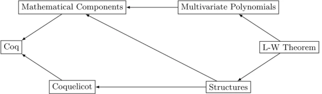
This means that our development is based on multiple libraries which were not meant to be used together. In Fig. 1, we show how the different libraries interact with each other. As the context for this proof is almost exactly the same as for the direct proof of e and π, you can refer to [3] for more details.
Multivariate Polynomials Mathematical Components
Coq
Coquelicot Structures
L-W Theorem
Fig. 1. Link between the different libraries
3
Following the Proof
Baker’s proof doesn’t actually prove Theorem 1 but rather a reformulation which we call Theorem 2. This reformulation provides the advantage of eliminating the study of linear and algebraic independence.
Theorem 2 (Baker’s reformulation). For any non-zero natural number l, any distinct algebraic numbers α1, . . . , αl and any non-zero algebraic numbers
β1, . . . , βl, we have:
β1eα1+ . . . + βleαl 6= 0 . (2)
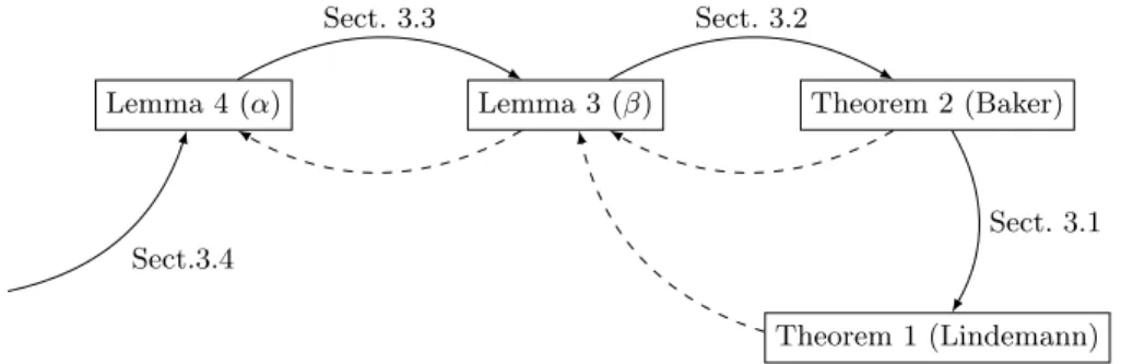
Its proof has 3 main steps. The first one focuses on the β’s and strengthens their hypothesis, using the first lemma (Lemma 3). The second one deals with the α’s and adds some conditions on them, showed in Lemma 4. The final part actually deals with the last lemma and proves it. We will present the ideas of these different steps in the following subsections.
In Fig. 2, the dashed arrows are the trivial implications that are not proved in this paper, as we focus on the proof of the Lindemann-Weierstrass theorem.
Theorem 2 (Baker) Lemma 3 (β) Lemma 4 (α) Theorem 1 (Lindemann) Sect. 3.1 Sect. 3.2 Sect. 3.3 Sect.3.4
Fig. 2. Implications between the different theorems and lemmas
3.1 Baker’s Reformulation
In this subsection, we prove that the Lindemann-Weierstrass theorem is at least as strong as Baker’s reformulation (previously called Theorem 2).
As the notations in Sect. 2 cover our needs, we can immediately give the Coq translation of Theorem 2, and notice the change on l: to avoid any problem later on, we explicitly state that the tuple is not empty, as its size is l.+1. It should be noted that the conditions that the α’s must be distinct is seen as the injectivity of the function alpha from ’I l.+1 to complexR.
Theorem LindemannBaker :
forall (l : nat) (alpha : complexR^l.+1) (a : complexR^l.+1), injective alpha →
(forall i : ’I_l.+1, alpha i is_algebraic) → (forall i : ’I_l.+1, a i != 0) →
(forall i : ’I_l.+1, a i is_algebraic) → (Cexp_span a alpha != 0).
In order to prove this reformulation is at least as strong as Theorem 1, we need to recall some definitions around multivariate polynomials. The support of a multivariate polynomial p is the set of all the monomials which have a non-zero coefficients, and is written msupp p in Coq. Finally, it is worth noticing that when one evaluates a monomial on a set of exponential of numbers, one obtains the exponential of a linear combination of these numbers.
As shown below, the proof of the implication of the Lindemann-Weierstrass theorem by Baker’s reformulation is pretty straightforward.
Proof. Let us call t the tuple of the support of p, alpha (resp. beta) the tuple of the evaluation of the monomials of t on the exponentials of a (resp. the coefficients of the monomials of t in p). We can then recognize an exp-linear combination: we prove the following equality and rewrite it.
P.@[finfun (Cexp \o a)] = Cexp_span beta alpha.
By applying Theorem 2, we are left with all its hypothesis to prove. All of them are almost instantaneous except the injectivity of alpha. To prove this last bit, it suffices to unfold alpha so that we obtain an equality between two linear combinations of the a, which can we reduced to a single linear combination.
\sum_(k < n) (((t i) k)%:R - ((t j) k)%:R) * a k != 0
By linear independence, and unicity of the support of a polynomial, the proof
is finished. ut
3.2 Simplifying the β’s
The goal of the first part of Baker’s proof is to show that we can assume, without loss of generality, that the β’s are integers. Thus, this subsection gives some insights about the set of roots of a polynomial, the minimal polynomial, a total order on the complex and the formalization of the maximum of a tuple. With all these facts, we prove that Lemma 3 below implies Theorem 2.
Lemma 3. For any non-zero natural number l, any distinct algebraic numbers α1, . . . , αl and any non-zero integers β1, . . . , βl, we have:
β1eα1+ . . . + βleαl 6= 0 . (3)
The main difference between the mathematical statement and the Coq one is that we replace the condition on l to be non-zero by the explicit value l.+1.
Lemma wlog1 :
(forall (l : nat) (alpha : complexR^l.+1) (a : complexR^l.+1), injective alpha →
(forall i : ’I_l.+1, alpha i is_algebraic) → (forall i : ’I_l.+1, a i != 0) →
(forall i : ’I_l.+1, a i \is a Cint) → (Cexp_span a alpha != 0)).
To explain the proof, we need some definitions about symmetric polynomials and minimal polynomials. A multivariate polynomial is said to be symmetric if it is left unchanged by any permutation of its variables. For instance, the following polynomial is symmetric, but its first half isn’t.
X3Y2Z + X2Y Z3+ XY3Z2+ X3Y Z2+ X2Y3Z + XY2Z3 . (4) The fundamental theorem of symmetric polynomials states that any symmet-ric polynomial in a ring IK can be obtained from a particular set of symmetsymmet-ric polynomials using only addition, multiplication, and multiplication by coeffi-cients in the ring IK. As we shall develop more on this topic later, let us just remark that as a consequence of this theorem, we have that for any symmetric polynomial whose coefficients are in IK, its evaluation on the set of roots of a polynomial is in IK.
To more easily track the set of roots of a polynomial, we gave ourselves a small definition, which expresses that a set f is the set of roots of a polynomial. To be more general, we consider an archimedean closed field T with a norm and partial order, a predicate S and say that the polynomial whose roots are exactly f has all its coefficients in S when multiplied by a number c.
(f \is a set_roots S c) =
((c *: \prod_(x <- enum_fset f) (’X - x%:P)) \is a polyOver S).
In our case, the predicate will be Cint and the field complexR. Once more, as we can’t recognize the rational numbers among the complex, we workaround this problem by specifying a multiple (c) of the expected least common multiple of the denominator of all the coefficients. The negative point of having one more parameter is once again largely compensated by the gain in ease of proof from a boolean predicate.
The minimal polynomial of an algebraic complex number x is the polynomial of smallest degree which has x as a root, whose coefficients are in Q and whose leading coefficient is 1 (we also say monic). We defined two related notions for the minimal polynomial: the one whose coefficients are in ZZ, and the one already embedded in the complex.
The first one, polyMinZ, is the irreducible, separable polynomial whose co-efficients are in int, whose zcontents (the greatest common divisor of all its coefficients with the same sign as the leading coefficient) is 1, and which divides exactly all the polynomials which have x as a root. It corresponds to the minimal polynomial multiplied by the least common multiple of the denominators of all its coefficients, and if needed, by −1 so that the leading coefficient is positive.
{p : {poly int} | [∧ (zcontents p = 1),
irreducible_poly p, separable_poly (map_poly ZtoC p)
& forall q : {poly int}, root (map_poly ZtoC q) x = (p %| q)]}.
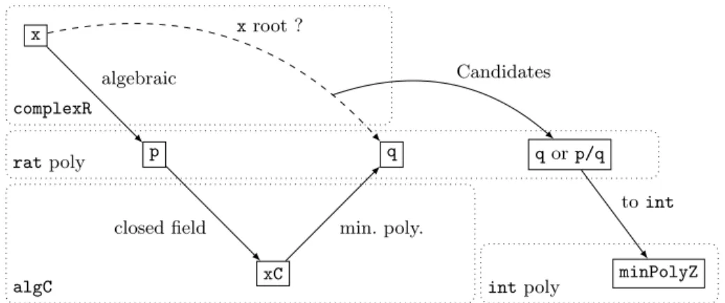
To prove the existence of such a polynomial, we used the fact that any number of type algC has a minimal polynomial over rat. As shown in Fig. 3, from an algebraic complex number x, we obtain a polynomial p which has x as a root. We can then proceed by recurrence on the degree of p to prove the existence
of the minimal polynomial of x: if it is below or equal to 2, we already have a candidate for the minimal polynomial. From this point, we extract a root xC in algC of the polynomial p embedded in algC, and call its minimal polynomial q. If x is a root of q, we found a candidate for its minimal polynomial. If not, then q divides p, and we obtain a new polynomial with coefficients in rat with a smaller size and which has x as a root. By recurrence, we obtain a candidate. Once we have a candidate, we have to transform it to be in int instead of rat, by multiplying it by the least common multiple of the denominators of all its coefficients. x p xC q q or p/q minPolyZ algebraic
closed field min. poly. x root ?
Candidates
to int complexR
rat poly
algC int poly
Fig. 3. Existence of a minimal polynomial
Proof (Lemma 3 =⇒ Theorem 2). We proceed by contrapositive, so we assume we have some l, α’s and β’s that respect Theorem 2’s assumptions but contradict its conclusion: the linear combination of the β’s and the exponentials of α’s is considered equal to 0. Every β is algebraic: for each k which ranges from 1 to l, we call Bk the set of roots of the minimal polynomial of βk. Then, we multiply
all the expressions obtained by letting the βk’s to run independently through
the Bk’s in the left-hand side of (2).
Y β0 1∈B1 · · · Y β0 l∈Bl (β10eα1+ . . . + β0 le αl) = 0 . (5)
Finally, (5) is symmetric with respect to each Bk so that the new coefficients
of the linear combination are rationals. It then suffices to multiply by the least common multiple of the denominators to ensure the new β’s are integers. ut In this proof, we can notice three main problems. In usual mathematical practice, we don’t even bother checking if there is at least one new β and α to contradict Lemma 3. Secondly, we recognize an expression as symmetric and then directly state that the result is what we expected. Actually, we are supposed to
begin by showing it is a symmetric polynomial evaluated on some numbers, then continue by applying the fundamental theorem of symmetric polynomials and end by verifying we obtain a Q-exp-lin combination. Finally, even the application of the theorem is misleading: we have to apply it for each Bk.
The first point can be resolved by following the highest α according to the lexical ordering on complex numbers following the real part and then the imagi-nary part:
Definition letc x y :=
(’Re x < ’Re y) || ((’Re x == ’Re y) && (’Im x <= ’Im y)).
In order to follow the highest of the α’s, we define the maximum of a tuple. This is the repeated use of the maxc operation on the tuple, which evokes the bigop module. The structure (complexR, maxc) is not equipped with a monoid structure and we cannot use directly the big operations provided by the MathComp library. In the case of a non-empty tuple f, we invoke the sequence case whose default value is the first value of the tuple (f ord0), and whose sequence is the sequence value of the tuple (codom f).
Definition bmaxf n (f : complexR^n.+1) := bigmaxc (f ord0) (codom f).
The third point can be resolved by changing a little bit the proof. Instead of letting each βk to run only within Bk, they can now run through the whole
B =Ul
k=1Bk, seen as a multiset. Expression (5) is then changed into:
Y β0 1∈B · · · Y β0 l∈B (β10eα1+ . . . + β0 le αl) = 0 . (6)
It presents two immediate benefits. First, (6) is now completely symmetric in the β’s, which means we now only have to use the fundamental theorem of symmetric polynomials once. Secondly, it makes the expression clearer, and thus, more convincing. Finally, we can notice that the products in (6) can be replaced by a single product sign over the l-tuples of elements of B.
For the second point, we can identify explicitly the left-hand side of (2) with a multivariate polynomial whose coefficients are also multivariate polynomials evaluated on the right points: the first set of indeterminates represents the β’s, the second set is used to hide the exponentials and verify that, in the end, we still obtain a linear combination of rationals and exponentials. For instance, (6) is changed into the following, where L.+1 is the cardinal of B.
((\prod_(f : ’I_L.+1 ^ l.+1) \sum_(i : ’I_l.+1) ’X_i *: ’X_(f i)) .@[finfun ((@mpolyC l.+1 complexR_ringType) \o beta)])
.@[finfun (Cexp \o alpha)] = 0.
We can also notice that Lemma 3 is a direct consequence of the Lindemann-Weierstrass theorem.
3.3 Simplifying the α’s
The second and third steps in Baker’s proof both revolve around the same new lemma which strengthens the conditions on the α’s. But, we need some last definitions to be able to write it.
First of all, a partition of a set S is a set of sets such that none of its elements is the null set, all of its elements are disjoint, and the union of all its elements is exactly S. For instance, {{1, 3, 6}, {2}, {4, 5}} is a partition of {1, 2, 3, 4, 5, 6}. In MathComp, the notion already existed and is based on the null set (set0), the union of all its parts (cover P) and trivIset which is a predicate that treats the disjoint condition by studying the cardinal of the parts of P.
Definition partition (T : finType) (P : {set {set T}}) (D : {set T}) := [&& cover P == D, trivIset P & set0 \notin P].
Secondly, two complex numbers are called conjugates if they are roots of a same minimal polynomial. In particular, in order to find a minimal polynomial, we need at least one of those numbers to be algebraic. In this case, an algebraic number x and a complex number y are conjugates if y is a root of the minimal polynomial of x.
Lemma conjOfP (x y : complexR) (x_alg : x is_algebraic) : reflect (y \is a conjOf x_alg) (root (polyMin x_alg) y).
We also say a set of conjugates is complete if it is exactly the set of all the roots of a minimal polynomial. For instance, {√32, e2iπ
3 3
√
2, −e2iπ3 3
√ 2} is a complete set of conjugates. Formalizing this property with a boolean predicate leads to a strange definition which once again uses an additional parameter c with the same role. In particular, given a complex c and a set f of complex numbers, our definition checks if P := c *: \prod (x <- enum fset f) (’X - x%:P) is non-zero, non-constant and only has integer coefficients, and from the proofs of these three statements, it constructs the minimal polynomial of a root of P. Then, it suffices to check if these two polynomials are equal up to an integer multiplication. In particular, any complex in a complete set of conjugates is algebraic.
Lemma setZconj_algebraic (c x : complexR) (f : {fset complexR}) : x \in f → f \is a setZconj c → x is_algebraic.
Lemma 4. For any non-zero natural number l, any distinct algebraic numbers α1, . . . , αl and any non-zero integers β1, . . . , βl, such that the α’s can be grouped
into a partition P , if for each part in P , the α’s form a complete set of conju-gates, and on each part in P , the β’s are constant, then:
β1eα1+ . . . + βleαl 6= 0 . (7)
With the previously introduced notation, we obtain the following lemma in Coq.
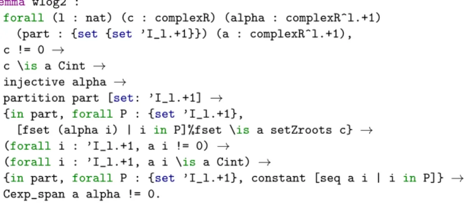
Lemma wlog2 :
forall (l : nat) (c : complexR) (alpha : complexR^l.+1) (part : {set {set ’I_l.+1}}) (a : complexR^l.+1), c != 0 →
c \is a Cint → injective alpha →
partition part [set: ’I_l.+1] → {in part, forall P : {set ’I_l.+1},
[fset (alpha i) | i in P]%fset \is a setZroots c} → (forall i : ’I_l.+1, a i != 0) →
(forall i : ’I_l.+1, a i \is a Cint) →
{in part, forall P : {set ’I_l.+1}, constant [seq a i | i in P]} → Cexp_span a alpha != 0.
To continue the proof of the Lindemann-Weierstrass theorem, we need to prove that Lemma 4 implies Lemma 3. Its proof follows the same steps as the proof in Sect. 3.2 so we won’t give too much details. The main differences and sources of difficulties between the two proofs can be found in Fig. 4. They come from the fact that we need to be far more specific in each argument.
α β
A B
poly poly of poly
polys poly
new α/β new α/β
partition separable poly with at
least the α’s as roots
product of all the minimal polynomial of the β’s
on injective functions An
on functions Bn
decomposition on monomial
symmetric polynomials evaluation
conjugates
roots
symmetry
product of exp-linear combinations
evaluation, eliminate the duplicates,
coefficients not null
Lemma 4 =⇒ Lemma 3 Lemma 3 =⇒ Theorem 2
Fig. 4. Comparison of the proofs of Sect.3.3 (left) and Sect.3.2 (right)
For instance, in Sect. 3.2, we introduced the fundamental theorem of sym-metric polynomials. Here, we need a more precise version that states that any
symmetric polynomial in a ring IK can be obtained as a IK-linear combination of a particular set of symmetric polynomials: the monomial symmetric polyno-mials. Each one is exactly the smallest symmetric polynomial of a monomial Xk1
1 X k2
2 . . . Xnkn, that is the sum of all the monomials X k1 σ(1)X k2 σ(2). . . X kn σ(n)that
can be obtained from all the permutations σ of the indeterminates. In Coq, we called them mmsym x or ’m x if x is a monomial.
3.4 Proving the Final Lemma
The final part of the proof uses even more precise arguments around multivariate polynomials and symmetry.
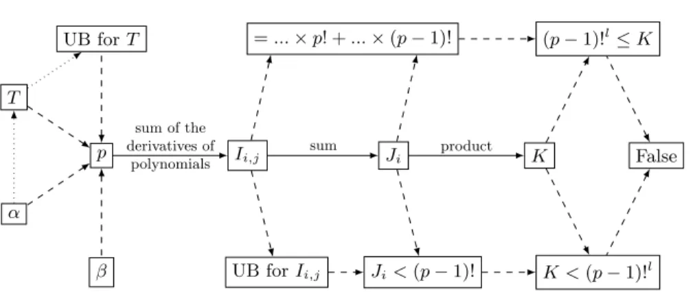
Proof. To actually prove Lemma 4, which corresponds to the third part of Baker’s proof, we proceed by contradiction. We then need to introduce many notations and a big enough prime number p. This p only depends on the values of the α’s and β’s, and must be an upper bound (UB) of a certain polynomial T on [0; 1]. Once it is defined, we construct other polynomials and values I, J and K, as shown in Fig. 5 and study them in two ways. First, with algebra, we can show they have some properties of divisibility which lead to a lower bound for K. Then, as I can be recognized as an integral of a function of T , we can find an upper bound, and consequently, an upper bound for K, too. Finally, we combine both inequations involving K:
(p − 1)!n≤ K < (p − 1)!n . (8)
This is a logical contradiction which completes the proof. ut
α T β UB for T p Ii,j Ji K False UB for Ii,j Ji< (p − 1)! K < (p − 1)!l = ... × p! + ... × (p − 1)! (p − 1)!l≤ K sum of the derivatives of polynomials sum product
Fig. 5. Proof structure of Lemma 4
This proof follows the same steps as the common lemma of the transcendence of e and π up until the results on J . In the last few different steps which are only in the algebra part, Baker proposes to impose being algebraic integers on
the α’s and then speaks of divisibility of algebraic integers by natural numbers. Because of the path chosen in the common lemma proof, we can finish the proof without ever explicitly using algebraic integers.
The proofs of divisibility on K relies heavily on repeated uses of the fun-damental theorem of symmetric polynomials. In fact, K is the evaluation of a multivariate polynomial Km on the α’s. For each part of the partition P , Km
is symmetric on the subset of indeterminates of the part but not fully symmet-ric. This means that the theorem can not be applied directly on the full set of indeterminates, but repeatedly on each subset of indeterminates corresponding to a part of the partition, that is on a subset of indeterminates which make Km
symmetric and corresponds to a complete set of conjugates. All the indetermi-nates must be considered once and only once, hence the need for a partition on complete set of conjugates.
We formalized a predicate symmetric for indicating if a multivariate poly-nomial is symmetric on a given subset of its indeterminates in the same way as a fully symmetric polynomial: it must be equal to itself on any permutation of this subset of indeterminates. This was done with an already existing predicate perm on on permutations that states that outside the subset, the permutation maps a value to itself.
Thanks to this predicate and extensions of other notations such as the small-est symmetric polynomial containing a monomial, we were able to obtain a new formalized corollary of the fundamental theorem of symmetric polynomials. Lemma 5. Given a natural number m, a m-tuple l of unique complex numbers, a m-variate polynomial p whose coefficients are rationals, and P a partition of {1, . . . , m}, if p is symmetric on each part of P for each part of P , the corre-sponding l’s form a complete set of conjugates, then P (l1, . . . , lm) is rational.
This can be generalized in Coq to a closed field T (instead of C) and a boolean predicate kS (instead of rational) compatible with ring operations.
partition P [set: ’I_m.+1] → injective l →
{in P, forall Q : {set ’I_m.+1},
[fset l i | i in Q]%fset \is a set_roots kS c} → p \is a mpolyOver m.+1 kS →
{in P, forall Q, p \is (@symmetric_for _ _ Q)} → c ^+ (msize p).-1 * p.@[l] \in kS.
4
Conclusion
4.1 Related Work
Concerning transcendance formalizations, this work is a follow-up of the proof of transcendence of e by Bingham [4] in HOL Light, and of the proofs of tran-scendance of e and π in Coq.
The work on multivariate polynomials is primarily based on a development made by Strub, and continued by Hivert who also formalized monomial sym-metric polynomials but relied upon the definitions of partitions of an integer. We prefered to have a self-sufficient definition which introduces the notion of the smallest symmetric polynomial containing a monomial. Nevertheless, we added a lemma to ensure the compatibility of both definitions.
To our knowlegdge, this is the first formalization of multivariate polynomials that are symmetric on a subset of their indeterminates. This is not really sur-prising as the main current use of multivariate polynomials consists in studying the Bernstein polynomials [15] in order to approximate polynomial inequalities. Moreover, it would be easier to separate the indeterminates in two sets (sym-metric or not) of indeterminates, rather than staying with a fixed number of indeterminates.
4.2 Future Work
In the future, the multivariate polynomial library will evolve to pick the inde-terminates differently, allowing the change of the number of indeinde-terminates to be far easier. This will probably change the statement of the corollary of the fundamental theorem of symmetric polynomials, and make its proof way easier. It could be interesting to try to formalize the same theorem using Galois theory as it is already formalized in Mathcomp, to compare the proofs. In the same spirit, proving the existence of an embedding from the algebraic complex numbers (type algC) to the complex numbers (type complexR) could offer a different view on the proof, with different definitions or different proofs. Never-theless, the construction of the complex numbers would still be necessary for the analysis part.
The next step could probably be to prove Baker’s theorem on the linear form of complex logarithms, as it is the basis for several developments derived from transcendence.
References
1. Formalization of the Lindemann-Weierstrass theorem in Coq. http://www-sop.inria.fr/marelle/lindemann/
2. Baker, A.: Transcendental number theory. Cambridge University Press (1990) 3. Bernard, S., Bertot, Y., Rideau, L., Strub, P.Y.: Formal proofs of transcendence
for e and pi as an application of multivariate and symmetric polynomials. In: Proceedings of the 5th ACM SIGPLAN Conference on Certified Programs and Proofs, 76–87. ACM (2016)
4. Bingham, J.: Formalizing a proof that e is transcendental. Journal of Formalized Reasoning 4(1), 71–84 (2011)
5. Boldo, S., Lelay, C., Melquiond, G.: Coquelicot: A user-friendly library of real analysis for Coq. Mathematics in Computer Science 9(1), 41–62 (2015)
6. Cohen, C.: Finmap library, http://github.com/math-comp/finmap
7. Cohen, C.: Formalized algebraic numbers: construction and first-order theory. Ph.D. thesis, Citeseer (2013)
8. Coq development team: The Coq proof assistant (2008), http://coq.inria.fr 9. Gonthier, G.: Formal proof–the four-color theorem. Notices of the AMS 55(11),
1382–1393 (2008)
10. Gonthier, G., Asperti, A., Avigad, J., Bertot, Y., Cohen, C., Garillot, F., Le Roux, S., Mahboubi, A., OConnor, R., Biha, S.O., et al.: A machine-checked proof of the odd order theorem. In: International Conference on Interactive Theorem Proving, 163–179. Springer (2013)
11. Hermite, C.: Sur la fonction exponentielle (1874)
12. Lang, S.: Algebra revised third edition. Graduate Texts in Mathematics 1(211). Springer (2002)
13. Lindemann, F.: ¨Uber die zahl π. Mathematische Annalen 20(2), 213–225 (1882) 14. Liouville, J.: Sur des classes tr`es-´etendues de quantit´es dont la valeur n’est
ni alg´ebrique, ni mˆeme r´eductible `a des irrationnelles alg´ebriques. Journal de math´ematiques pures et appliqu´ees, 133–142 (1851)
15. Mu˜noz, C., Narkawicz, A.: Formalization of a representation of Bernstein polyno-mials and applications to global optimization. Journal of Automated Reasoning 51(2), 151–196 (2013)
16. Weierstrass, K.: Zu Lindemann’s Abhandlung: ” ¨Uber die Ludolph’sche Zahl.”. Akademie der Wissenschaften (1885)