HAL Id: hal-02925519
https://hal.inria.fr/hal-02925519
Submitted on 30 Aug 2020
HAL is a multi-disciplinary open access
archive for the deposit and dissemination of
sci-entific research documents, whether they are
pub-lished or not. The documents may come from
teaching and research institutions in France or
abroad, or from public or private research centers.
L’archive ouverte pluridisciplinaire HAL, est
destinée au dépôt et à la diffusion de documents
scientifiques de niveau recherche, publiés ou non,
émanant des établissements d’enseignement et de
recherche français ou étrangers, des laboratoires
publics ou privés.
A Structure of Restricted Boltzmann Machine for
Modeling System Dynamics
Guillaume Padiolleau, Olivier Bach, Alain Hugget, Denis Penninckx, Frédéric
Alexandre
To cite this version:
Guillaume Padiolleau, Olivier Bach, Alain Hugget, Denis Penninckx, Frédéric Alexandre. A Structure
of Restricted Boltzmann Machine for Modeling System Dynamics. IJCNN 2020 - International Joint
Conference on Neural Networks, IEEE, Jul 2020, Glasgow, United Kingdom. pp.8. �hal-02925519�
A Structure of Restricted Boltzmann Machine for
Modeling System Dynamics
Guillaume Padiolleau
∗†‡§, Olivier Bach
∗, Alain Hugget
∗, Denis Penninckx
∗and Fr´ed´eric Alexandre
†‡§∗CEA-CESTA, Le Barp, France
Email: [email protected]
†INRIA Bordeaux Sud-Ouest, Talence, France
‡LaBRI, Universit´e de Bordeaux, Bordeaux INP, CNRS, UMR 5800, Talence, France §IMN, Universit´e de Bordeaux, CNRS, UMR5293, Bordeaux, France
Abstract—This paper presents a new approach for learning transition function in state representation learning (SRL) for control. While state-of-the-art methods use different deterministic neural networks to learn forward and inverse state transition functions independently with auto-supervised learning, we in-troduce a bidirectional stochastic model to learn both transition functions. We aim at using the uncertainty of the model on its pre-dictions as an intrinsic motivation for exploration to enhance the representation learning. More, using the same model to learn both transition functions allows sharing the parameters, which can reduce their number and should increase the embedding quality of the representation. We use a factored restricted Boltzmann machine (fRBM) based model, enhanced with dedicated struc-ture for learning system dynamics and transitions with shared parameters. The presented work focuses on building the structure of the bidirectional transition model for unsupervised learning. Our fRBM structure is directly inspired from physics interactions between inputs and outputs in reinforcement learning framework. We compare different training algorithms for learning the model that must be able to predict observable random variables to be used in SRL framework. Our structure is not restricted to any type of observable, nevertheless in this paper we focus on learning dynamics from the OpenAI Gym environment Swinging Pendulum. We show that the proposed structure is able to learn bidirectional transition function and performs well in prediction task.
Index Terms—Factored Restricted Boltzmann Machine, Unsu-pervised Deep Learning, State Representation Learning
I. INTRODUCTION
One of the overarching goals of reinforcement learning is to find efficient policies in problems with high dimensional data. This challenge heavily relies on finding a low dimensional, meaningful and topologically coherent space for representing sensory data often called state space [1]. This can be hand crafted by experts but it is highly desirable to learn it from data. In this case, learning is driven by finding causal structure in sensory data. Optimizing causal relationship associating state and action with the corresponding next state leads to a latent space achieving better control on the environment. In this framework state space is seen as a middle ground between encoding observations and encoding dynamics w.r.t. actions.
At first glance only minimization of next state prediction error from current state and action seems necessary. But few works [2], [3], [4] show that retrieving action from
current state and next state is recommended to achieve better performance. Yet to the best of our knowledge only feed forward neural networks are used to fit system dynamics. Hence inference on next state and action leads to duplicate networks and thus to extend the number of parameters.
Moreover, feed forward neural networks feature another drawback. Even if we can access prediction errors there is no way for finding uncertainty on prediction. However uncertainty can be a key factor for driving exploration with intrinsic motivation [5], providing information on novelty before real exploration i.e. before comparison with real state.
To override these problems we propose to use stochastic energy-based neural networks to fit system dynamics. An energy-based network is an implicit network that builds re-lationship between different flows of input. Thus allowing to infer on different ”inputs” with the same set of parameters. On its side a stochastic network enables estimation of uncertainty through sampling. From that perspective Restricted Boltzmann Machine [6], [7] is a natural candidate to fit system dynamics. In this paper we will focus on a network structure that links action and observations (before and after the action). We will not take into account coding and decoding parts which are necessary for state representation learning, leaving that for future work. Indeed, we are interested in dealing with the burden of trade-off between expressiveness and simplic-ity. Consequently, network structure was designed to mimic physical relationships without loss of generality, leading to a network with stable behavior which manages to fit complex transformations.
In section II we expose technical bases on Restricted Boltzmann Machine (RBM), its learning algorithms and its conditional version. Section III focuses on higher order Re-stricted Boltzmann Machine which extends RBM relationship beyond 2 ways. This is of particular interest for us as we need a three-way relation between action and states/observations (previous and next ones). Section IV shows related works in the fields of state representation learning and of dynamical system modeling with RBM. Then, section V describes our model and presents results obtained on processing observations from a swinging pendulum.
II. RESTRICTEDBOLTZMANNMACHINES, EXTENSIONS,
ANDCONTRASTIVEDIVERGENCE
We begin by providing background knowledge used in this paper. Firstly, Restricted Boltzmann Machines (RBMs) are introduced and detailed. Secondly, maximum likelihood practical methods for training RBMs are presented.
A. Restricted Boltzmann Machines
A RBM is an undirected graphical model based on energy that defines a joint probability distribution over an input layer of observed variables v, called visible, and a layer of latent variables h, called hidden. These layers are composed of stochastic units that can be binary (i.e. Bernoulli) or real-valued (i.e. Gaussian). This paper considers only Gaussian visible layers and Bernoulli hidden layers since our application requires real-valued visible vectors. The joint probability over v and h is defined by:
p(v, h) = exp(−E(v, h))/Z (1)
where Z is the partition function and E is the energy function defined by: E(v, h) = Nv X i (vi− bvi) 2 2σ2 i − Nh X j hjbhj − Nv,Nh X i,j vi σi hjwij (2)
where Nv and Nh are the number of units in the visible and
hidden layers, respectively; bv
i and bhj are biases of the ith
visible unit and the jth hidden unit, respectively; wij is the
weight of the connection, from matrix W, between the ith visible unit and the jth hidden unit, and σi, from the diagonal
matrix Σ, represents standard deviation of the ith visible unit. A straightforward way to obtain p(v) is to marginalize out h from (1):
p(v) = exp(−F (v))/Z (3)
where F (v) is the free energy, such that: F (v) = − logX h exp(−E(v, h)) = Nv X i (vi− bi)2 2σ2 i − Nh X j log(1 + exp(bhj + vTΣ−1W·j)) (4) RBMs are typically trained using a gradient ascent of the log-likelihood llh(θ) for given training vector v. By using (3) to get the log-likelihood and differentiating with respect to parameter θ, the gradient is:
−∂llh(θ) ∂θ = ∂F (v) ∂θ − X u ∂F (u) ∂θ p(u) (5)
The first term of (5) is called the positive gradient. It can be computed exactly, given an input vector v, by differentiating (4). This term raises the probability of data by minimizing the model energy. The second term of (5) is called the negativegradient, and is the expectation over p(v), the model distribution. It is intractable, but Markov chain Monte Carlo
methods can draw samples from the model distribution to estimate this gradient. As a matter of fact, units in RBM layers are conditionally independent, thus conditionals factorize and give a simple way to compute activation probabilities of the entire layer as:
p(h|v) = Nh Y j p(hj|v) = Nh Y j ¯ σ(bhj + vΣ−1W·j) (6) p(v|h) = Nv Y i p(vi|h) = Nv Y i N (vi; bvi + hW T ·iσi, σi2) (7)
where ¯σ(·) is the sigmoidal function, and N (x; µ, σ2) is the normal distribution on x with mean µ and standard deviation σ. Then it is possible to perform an efficient Gibbs sampling by iterating over (6) and (7) and get model distribution samples to approximate negative gradient.
B. Conditional Restricted Boltzmann Machines
First advance of RBMs with multiple visible layers is the conditional RBM (cRBM) [8], [9] that has two visible layers, one of which is used as a conditional layer and cannot be inferred. A cRBM models the conditional distribution p(v|c) where v is the visible vector modeled by the RBM, and c is the conditioning vector used to dynamically bias the RBM. The energy function is then defined as:
E(v, h|c) = Nv X i (vi− ˆbvi) 2σ2 i − Nh X j hjˆbhj− Nv,Nh X i,j vi σi hjwijvh (8) where ˆbv
i and ˆbhj are the dynamic biases from c:
ˆbv i = bvi + Nc X k ckwcvki (9) ˆbh j = b h j + Nc X k ckwchkj (10)
and Wvh, Wch, Wcvare the matrix of pairwise connections
between v and h, the transition matrix from c to h and the transition matrix from c to v respectively.
C. Contrastive Divergence
[10] introduces the first practical method to approximate the negative gradient of log-likelihood. The method proposes to train RBMs by starting a Gibbs chain at visible vec-tor of training data, and running it a few steps to get an estimation of samples drawn from model distribution. This method minimizes Contrastive Divergence (CD) which is a different function from negative log-likelihood. Indeed, CD is not minimizing any function, as shown in [11]. However it is widely used for training RBMs or other energy-based models since it produces good results in training.
D. Persistent Contrastive Divergence
The main issue of CD is the biased result of negative gradient estimation it provides. The Persistence Contrastive Divergence (PCD) method proposed in [12] aims at solving this problem. In PCD, the positive gradient is the same as in CD since it can be directly computed. But unlike CD, PCD keeps a persistent chain to estimate negative gradient. Many CD variants have been proposed to improve the negative gra-dient estimation as in [13], but almost all based on persistent chain [14], [15], [16].
However, PCD methods cannot be used for cRBMs. In cRBMs, each conditioning vector c leads to a unique distribu-tion p(v|c). Thus, it is impossible to use PCD-based methods to estimate negative gradient in learning. As reported in [9], sample from the model distribution p(v|c) will require to keep a persistent chain for each conditioning vector. But stochastic gradient descent requires mini-batches of training data to learn efficiently, then when the model revisits conditioning case, it has sufficiently changed for the persistent chain to be far from the current model distribution.
III. HIGHER-ORDERBOLTZMANNMACHINES
This section presents higher-order Boltzmann machines that are RBMs with a tensor of weights instead of a simple matrix to model interactions between multiple visible layers. Using multiple visible layers allows capturing joint or conditional distributions over multiple observed data.
A. Factored Restricted Boltzmann Machines
While cRBMs can model conditional probability distribu-tions p(v|c), it cannot model the inverse conditional p(c|v) because of the dynamic biases that are not bidirectional. A way to construct RBM models that are able to capture the joint distribution p(x, y) over two visible layers x and y is to use a gated RBM (gRBM) [17] defined by the energy function:
E(x, y, h) = −
Nx,Ny,Nh
X
i,j,k
wijkxiyjhk+ bias terms (11)
assuming Σx and Σy to be identity matrices for clarity.
Here, W is the three-way interaction tensor that learns the importance of correlations between x and y. This model can capture the full joint distribution as it is tri-directional, and inferring a layer is simpler since the input layer l must receive −∇lE from the other layers, before applying the
activation function. However gRBMs are very costly as the energy function is a sum over all layers. Time complexity for inference is O(NxNyNh) and due to the three-way tensor it
is not memory efficient with large inputs.
Recent studies on higher-order RBMs [18], [19], [20], [21] suggest that it is possible to use much less parameters by factorizing the multi-way interaction tensor to obtain a factored
RBM (fRBM) and reduce the order of parameters to O(N2).
From (11), the new energy function becomes:
E(x, y, h) = −
Nf
X
f
xWxf·f yWyf·fhW·fhf+ bias terms (12)
where Nf is the number of factors used to factorize the
multiplicative tensor. As the factorization only applies to interactions between layers, the bias terms remain unchanged. As in gRBMs, inference on layer l is done by sending the −∇lE to the activation function.
B. Training fRBMs
Since fRBMs have multiple visible layers, the CD method must be extended to estimate the negative gradient w.r.t. the model distribution p(x, y). Two main strategies exist to draw samples from the model distribution using Gibbs sampling. The main issue is that p(x, y|h) is intractable, thus the Gibbs sampler needs to estimate model samples using p(x|y, h), p(y|x, h), p(h|x, y).
1) Alternating CD: The first way consists in estimating p(x, y|h) by an alternating Gibbs sampling step: randomly sample a new visible vector from p(x|y, h) or p(y|x, h), sample from p(h|x, y), sample the other visible vector with previous samples, and then re-sample h from the two sampled visible vectors. This method requires to run only one chain to estimate the model distribution, making it computationally efficient. Because this algorithm alternates between sampling x and y in a single Gibbs step, we denote it as aCD for alternating CD.
2) Cyclic CD: The second way, introduced in [22] for gRBMs, consists in running one Gibbs chain for each visible layer. The algorithm makes a cycle over visible layers to sam-ple only from conditionals, then we denote it as cCD for cyclic CD. [22] suggests that cCD has better performance than aCD for gRBMs, thus probably for fRBMs. A variant of cCD was introduced in [20] (denoted SMcCD for Sequential Markov chain CD), where positive h are computed by setting to zero the visible layer sampled in negative phase of estimation, to perform better in prediction.
IV. RELATEDWORK
State Representation Learning (SRL) for control shows good results in learning meaningful representations that help strate-gies learning in reinforcement context [1]. Given observable vector ot, the representation model φ must learn a meaningful
representation st. For that purpose, it has to learn a causal
structure by finding out a transformation over time. From the encoding point of view, the use of a Variational Auto-Encoder (VAE) [23], [24] can lead to an uncertainty in the state space. [23] uses a pre-trained VAE with frozen variance in the dynam-ics learning phase, but the mixture density network combined with a Recurrent Neural Network (RNN) is able to give an uncertainty on prediction. [24] uses a simple linear model to modify mean and variance of encoder and decoder, leading to the same capacity for modeling uncertainty of prediction.
However, both models use feed forward network tuned to match only future observations. [2], [3] and [4] use forward and inverse models to obtain better results on representation space. Nevertheless, they are deterministic models that cannot predict uncertainty.
From RBM point of view, [19] and [20] are interested in learning transformations between temporal observations. Both of them focus on skeleton movement conditioned on activity label. Their studies show that fRBMs can learn multi-directional transition models, i.e. we can use a unique model to replace forward transition and inverse transition models. And since fRBMs are stochastic neural networks, they are less sensitive to representation noise during learning or inference phases. This paper does not deal with the final SRL system, but on the construction of a fRBM architecture for the bidirec-tional transition model. In the next section, we will see how our model differs from those proposed in [19] and [20].
The fRBM architecture proposed in [19] for transition learning uses three different three-way factors with one being totally conditional (i.e. hidden layer is not an input of this factor). This model can be hard to train due to the competition between all factors, and then needs different learning rates for each factored sub-model. The architecture proposed in [20] bypasses this issue by using one four-way factor between the four layers. But these two architectures are conditioning p(st+1|s<t+1, l) where label l remains constant for all time
steps, i.e. the model learns different modes of time series. Our problem is different since time series are trajectories where the next state st+1 depends on at and stwhich are changing
at each time step.
V. OURMODEL
A. Architecture
As our model will be used for SRL bidirectional transitions, we want the hidden layer h to encode the transformation of the current transition between current state st and next state
st+1 (corresponding to backward transition model), and to
encode the transformation implied by applying action at at
current state st. These two transformations need to be encoded
in h independently but in the same way. Thus we use one factor for each transformation. However, using a scalar value for at can be an issue for prediction: when action is zero
then the contribution from its factor to h is zero too due to multiplicative interactions only. In prediction phase st+1 is
initialized to zero, thus all factors have zero contribution to h. To avoid this situation, we enforce a dynamic bias from st
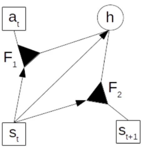
on h to always encode at least the current state. This results in the final architecture in Fig. 1, where the arrow symbol-izes directed connections (i.e. conditional connections), lines symbolize bidirectional connections, and triangles symbolize factors as three-way multiplicative interactions. Visible layers are represented with squares and hidden layer with a circle. Assuming for simplicity a unit standard deviation for at, st,
Fig. 1. Our architecture with visible layers (at,st,st+1) represented with
a square, and hidden layer h with a circle. Lines are for bidirectional connections, arrows for directional connections, and triangles are factors as three-way multiplicative connections. Hidden units must encode both the transformation between current state st and next state st+1, and the
transformation implied by applying action atin current state st, depending
on current state.
and st+1, the energy function of this model is:
E(at, st+1, h|st) = (at− ba)2 2 + Ns X j (st+1,j− bsj)2 2 − Nf1 X f1 atWaFf11· stW stF1 ·f1 · hW hF1 ·f1 − Nf2 X f2 st+1W st+1F2 f2 · stW st,F2 ·f2 · hW hF2 ·f2 − Nh X k hkˆbhk (13) where ba and bs are biases of at and st+1 respectively;
W·F1 and W·F2 are the factorization weights w.r.t. first and
second factor respectively; the dynamic bias is defined by ˆbh
k = b h
k + stB·k; and · corresponds to element-wise matrix
multiplication.
Inference in this model is simple for atand st+1since they
do not depend on each other directly, but more complex for h which takes contributions from both factors:
p(h|at,st+1, st) = ¯σ(atWaF1· stWstF1(WhF1)T + stWstF2· st+1Wst+1F2(WhF2)T + ˆbh) (14) p(at|h, st) = N (at; ba+ hWhF1· s tWsF1(WaF1)T, 1) (15) p(st+1|h, st) = N (st+1; bs+ hWhF2· s tWsF2(Wst+1F2)T, 1) (16) B. Training
Using equations (14), (15) and (16), we can perform Gibbs sampling to approximate samples from model distribution.
Whatever the CD method used, the form of the free energy gradients is the same. As examples, we give gradients w.r.t. WaF1, B and bs: ∆WaF1 1f1 ∝hat Ns X j st,jWjfst1F1 Nh X k hkWkfhF11i0 − hat Ns X j st,jWjfst1F1 Nh X k hkWkfhF11ik (17) ∆Bik∝ hst,ihki0− hst,ihkik (18) ∆bsj∝ hst+1,ji0− hst+1,jik (19)
where h·i0and h·ik denote expectations under data distribution
and estimated model samples after k Gibbs sampling steps. In general, the form of the CD w.r.t. θ is given by
∆θCDk∝ h ∂E(at, st+1, h|st; Θ) ∂θ i0−h ∂E(at, st+1, h|st; Θ) ∂θ ik (20) To approximate the negative gradient of CD, we can use all methods except persistent ones because of our conditioning. Indeed since the two distributions p(at|st, h) and p(st+1|st, h)
are conditionally independent we can use classical CD by alternating Gibbs sampling on h and both visible layers. Other methods such as aCD, cCD or its variant SMcCCD have been tested.
VI. EXPERIMENTS AND RESULTS
A. OpenAI Gym Environment
OpenAI Gym [25] is a toolkit for reinforcement learning which provides multiple environments to interact with. Each environment is designed to take an action in input and to return an observation. We do not train any agent in our experiments. Instead, provided environments help to collect data from simulated physics. The environment used for our experiment is Swinging Pendulum, which takes in input a scalar action (torque applied on the pendulum) in [−2, 2] in arbitrary units and returns an image of the pendulum as observable, also including the action represented with a circular arrow. We modified the environment to return an arrow reflecting the radial speed of the pendulum as we do not want the image to contain information about action.
To build the dataset, we ran 300 trajectories with initial angle state distributed from −π to π in order to ensure visiting all angles. Actions are sampled from uniform distribution on [−2, 2] with a trajectory length of 50 time steps to get most of possible actions. The dimensionality of images is reduced from 3x500x500 to 1x35x35, even if this remains a large dimensionality, and we standardize image values.
B. Learning
The model and all different training algorithms based on CD are implemented using Tensorflow [26] to run them on GPUs. All trained models have the same number of hidden units Nh= 100, and same number of factors NF1 = 150 and
NF2 = 250. For all experiments, we use a learning rate of
η = 10−4 to keep a bounded reconstruction error as explained
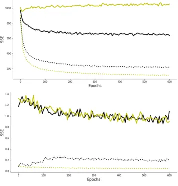
Fig. 2. SSE of reconstructions (dashed lines) and predictions (solid lines) during training for SMcCD (black) and aCD (yellow) (CD and cCD curves are almost superimposed to aCD curve). (Top) SSE for st+1. (Bottom) SSE
for at.
in [27] and [20]. The sparsity target for h is set to a mean activation of 0.5, in order to revive hidden units that are never active and suppress those that are always active [27], with gain β = 10−2. We use a weight cost using L2-norm with
gain γ = 10−3 and weight normalization for factor weights after each parameter update. But we do not use momentum because it leads to instabilities from the very large gradients it creates at the start of learning. An improvement could be a momentum schedule starting from low to higher value. This results in the following general update rule for parameter θ:
θ = θ + η(∆θCDk− γ 2 ∂kθk2 2 ∂θ − βh∂E(at, st+1, (h − 0.5 · 1)|st) ∂θ i0) (21)
Note that for all biases there is no L2-norm derivative, and for
visible biases there is no sparsity constraint. During learning we use k = 10 Gibbs sampling steps for all CD variants but for the SMcCD which uses k = 1 because it is less stable with high values of k. We set a non-learnable unit variance for both at and st+1.
C. Results
To perform reconstruction and prediction tasks, we use the method from [9]. To get good samples, we run k Gibbs sampling steps, compute free energy for the k samples, and take the sample which has the lowest free energy. During learning we sample model distribution, but for prediction we use meanfield inference (i.e. we use mean of probabilities).
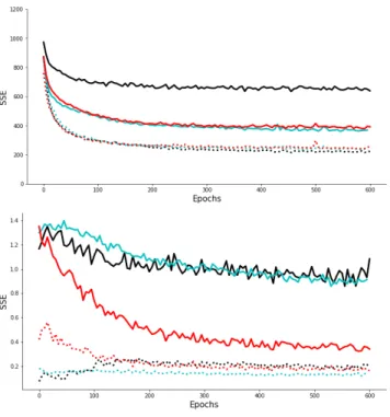
Fig. 3. SSE of reconstructions (dashed lines) and predictions (solid lines) during SMcCD training for 1 observed time step without gain on at(black),
5 observed time steps without gain on at(cyan) and 5 observed time steps
with a gain on at(red). (Top) SSE for st+1. (Bottom) SSE for at.
To follow convergence during learning, we use sum squared error (SSE) for reconstructions and predictions on a test set of trajectories. We choose SSE rather than mean squared error to get a more accurate view of learning process. SSE is tested after each epoch and averaged every 5 epochs. Fig. 2 shows learning curves of the four tested CD methods. CD, aCD, and cCD have similar behaviors: a good score of reconstruction but bad prediction scores. Although models trained with these methods are able to capture dependencies since they almost re-construct perfect samples (even on denoising tasks that we do not show here because it is not our purpose), they are unable to predict st+1or at. SMcCD has been designed to perform well
on prediction tasks and shows much better results. However, all training algorithms give the same performance on scalar at
predictions.
As SMcCD is the best training method for prediction, we go further with it and test it with different number of previously observed steps tN for st and at, i.e. image st becomes a
vector of images st−tN+1:t and scalar at becomes vector
at−tN+1:t. We compare SSE on st+1 and at during training
for tN = {1, 3, 5}, and show results in fig. 3 for tN = 1 and
tN = 5 in black and cyan respectively. Note that for at−tN+1:t,
we actually clamp the whole vector except at, i.e. the last time
step we want to reconstruct or predict. Fig. 3 (Top) shows how the number of observed time steps impacts prediction error on st+1. As expected, with multiple observed time steps the
model reaches better prediction performance. But it does not seem to affect prediction performance for at shown in fig. 3
TABLE I
SSEONst+1PREDICTION FOR DIFFERENT VALUES OFtNANDg
g = 1 g = 5 g = 10 tN= 1 637.80 635.33 599.51
tN= 3 434.84 476.12 417.89
tN= 5 368.34 390.95 354.88
TABLE II
SSEONatPREDICTION FOR DIFFERENT VALUES OFtNANDg g = 1 g = 5 g = 10 tN= 1 1.08 0.87 0.91
tN= 3 0.87 0.45 0.55
tN= 5 0.91 0.34 0.46
(Bottom, black & cyan). Nonetheless, during training, negative gradient w.r.t. atis estimated by sample p(at|h, st) with unit
standard deviation. We can use a lower standard deviation to get better performance, but this could cause gradient explosion from multiplications by inverse standard deviation. A trick to virtually reduce the model standard deviation is to apply a gain g on the input vector. But it can lead to imbalanced contributions between stand atif magnitudes are too different.
We trained model with SMcCD, tN = 1, 3, 5, and g = 1, 5, 10.
Table I shows SSE on st+1 predictions, and table II shows
SSE on at predictions at epoch 600. For tN = 1, it shows
that the value of the gain g does not have strong influence on predictions capabilities for both atand st+1. But interestingly,
for higher values of tN, the gain has an influence on both
at and st+1 predictions. Table I shows that a higher gain
helps model to have better prediction performance on st+1.
However, table II shows that a medium gain gives better prediction performances for at. As we are looking for good
performance on both predictions, we refer to model trained with SMcCD, tN = 5 and g = 5 as best model. It has the
best performance on at predictions, though it has the worst
performance on st+1 predictions for tN = 5, levels of SSE
are flatter and choosing any g has less impact.
For comparison, we show in fig. 5 and fig. 4 at and st+1
predictions respectively. For both, we compare our best trained model, model trained with tN = 1 and g = 1, and the ground
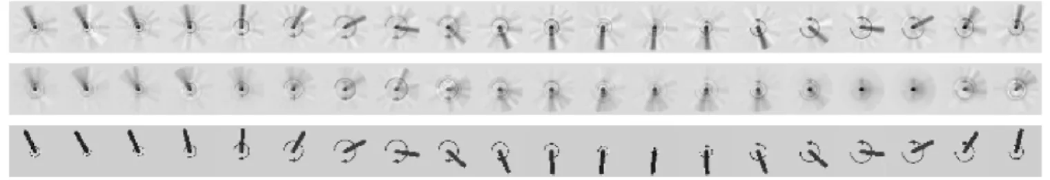
truth. Fig. 4 shows st+1 predictions for 20 time steps of our
best model (Top), the other model (Middle), and ground truth (Bottom). We do not show predictions from the model trained with other CD methods since our best model outperforms the other on prediction quality. Fig. 5 shows at predictions of
our best model in red, from the other model in cyan, and ground truth in black. The best model does not give always a perfect prediction, but wrong values stay not too far from ground truth, whereas the other model is not able to predict any of the ground truth action values.
VII. CONCLUSIONS ANDFUTUREWORK
We have presented a new fRBM architecture which is able to learn a bidirectional transition model without any supervision, with good results even with high dimensional data. The two independent factors of this fRBM encode in
Fig. 4. Images of st+1for 20 consecutive time steps of a trajectory. (Top) Meanfield predictions from best learned model with SMcCD, tN= 5 and g = 5.
(Middle) Meanfield predictions from model trained with SMcCD, tN= 1 and g = 1. (Bottom) Ground truth.
Fig. 5. Value of atfor 50 consecutive time steps of a trajectory. Red dashed
line is meanfield prediction from best learned model with SMcCD, tN = 5
and g = 5. Cyan dashed line is meanfield prediction from model trained with SMcCD, tN= 1 and g = 1. Black solid line is ground truth.
the same way a transition coming from different data views, referring to forward and inverse transitions. Unlike previously presented energy-based transition models based on fRBM [19], [20], this architecture aims to provide a more natural modeling of physics. In the context of SRL, this bidirectional model may simplify the learning by replacing both forward and inverse models used to constrain the representation. Our results focus on a given environment, however the proposed fRBM structure can apply more generally to any environment but only to transition learning with system dynamics modeling.
In future research, we will work towards interfacing this model with RBM-based auto-encoder to constrain the learning of meaningful representation in a fully unsupervised fashion. It will require modifying a part of SRL framework, since it uses gradient back-propagation through all networks, to use it with CD-like training algorithm.
REFERENCES
[1] T. Lesort, N. D´ıaz-Rodr´ıguez, J.-F. Goudou, and D. Filliat, “State representation learning for control: An overview,” Neural Networks, 2018.
[2] D. Pathak, P. Agrawal, A. A. Efros, and T. Darrell, “Curiosity-driven exploration by self-supervised prediction,” in Proceedings of the IEEE Conference on Computer Vision and Pattern Recognition Workshops, 2017, pp. 16–17.
[3] W. Duan, “Learning state representations for robotic control. m,” Ph.D. dissertation, Thesis, 2017.
[4] A. Zhang, H. Satija, and J. Pineau, “Decoupling dynamics and reward for transfer learning,” arXiv preprint arXiv:1804.10689, 2018.
[5] P.-Y. Oudeyer, F. Kaplan, and V. V. Hafner, “Intrinsic motivation systems for autonomous mental development,” IEEE transactions on evolutionary computation, vol. 11, no. 2, pp. 265–286, 2007. [6] P. Smolensky, “Parallel distributed processing: Explorations in the
microstructure of cognition, vol. 1. chapter information processing in dynamical systems: Foundations of harmony theory,” MIT Press, Cambridge, MA, USA, vol. 15, p. 18, 1986.
[7] Y. Freund and D. Haussler, “Unsupervised learning of distributions on binary vectors using two layer networks,” in Advances in neural information processing systems, 1992, pp. 912–919.
[8] G. W. Taylor, G. E. Hinton, and S. T. Roweis, “Modeling human motion using binary latent variables,” in Advances in neural information processing systems, 2007, pp. 1345–1352.
[9] V. Mnih, H. Larochelle, and G. E. Hinton, “Conditional restricted boltzmann machines for structured output prediction,” arXiv preprint arXiv:1202.3748, 2012.
[10] G. E. Hinton, “Training products of experts by minimizing contrastive divergence,” Neural computation, vol. 14, no. 8, pp. 1771–1800, 2002. [11] I. Sutskever and T. Tieleman, “On the convergence properties of contrastive divergence,” in Proceedings of the thirteenth international conference on artificial intelligence and statistics, 2010, pp. 789–795. [12] T. Tieleman, “Training restricted boltzmann machines using
approxima-tions to the likelihood gradient,” in Proceedings of the 25th international conference on Machine learning. ACM, 2008, pp. 1064–1071. [13] E. Romero, F. Mazzanti, J. Delgado, and D. Buchaca, “Weighted
contrastive divergence,” Neural Networks, vol. 114, pp. 147–156, 2019. [14] T. Tieleman and G. Hinton, “Using fast weights to improve persistent contrastive divergence,” in Proceedings of the 26th Annual International Conference on Machine Learning. ACM, 2009, pp. 1033–1040. [15] G. Desjardins, A. Courville, and Y. Bengio, “Adaptive parallel tempering
for stochastic maximum likelihood learning of rbms,” arXiv preprint arXiv:1012.3476, 2010.
[16] R. Salakhutdinov, “Learning deep boltzmann machines using adaptive mcmc,” in Proceedings of the 27th International Conference on Machine Learning (ICML-10), 2010, pp. 943–950.
[17] R. Memisevic and G. Hinton, “Unsupervised learning of image trans-formations,” in 2007 IEEE Conference on Computer Vision and Pattern Recognition. IEEE, 2007, pp. 1–8.
[18] R. Memisevic and G. E. Hinton, “Learning to represent spatial trans-formations with factored higher-order boltzmann machines,” Neural computation, vol. 22, no. 6, pp. 1473–1492, 2010.
[19] G. W. Taylor and G. E. Hinton, “Factored conditional restricted boltz-mann machines for modeling motion style,” in Proceedings of the 26th annual international conference on machine learning. ACM, 2009, pp. 1025–1032.
[20] D. C. Mocanu, H. B. Ammar, D. Lowet, K. Driessens, A. Liotta, G. Weiss, and K. Tuyls, “Factored four way conditional restricted boltz-mann machines for activity recognition,” Pattern Recognition Letters, vol. 66, pp. 100–108, 2015.
[21] K. Li, J. Gao, S. Guo, N. Du, X. Li, and A. Zhang, “Lrbm: A restricted boltzmann machine based approach for representation learning on linked data,” in 2014 IEEE International Conference on Data Mining. IEEE, 2014, pp. 300–309.
[22] D. Luo, Y. Wang, X. Han, and X. Wu, “A cyclic contrastive divergence learning algorithm for high-order rbms,” in 2014 13th International Conference on Machine Learning and Applications. IEEE, 2014, pp. 80–86.
[23] D. Ha and J. Schmidhuber, “World models,” arXiv preprint arXiv:1803.10122, 2018.
[24] H. Van Hoof, N. Chen, M. Karl, P. van der Smagt, and J. Peters, “Stable reinforcement learning with autoencoders for tactile and visual data,” in 2016 IEEE/RSJ International Conference on Intelligent Robots and Systems (IROS). IEEE, 2016, pp. 3928–3934.
[25] G. Brockman, V. Cheung, L. Pettersson, J. Schneider, J. Schul-man, J. Tang, and W. Zaremba, “Openai gym,” arXiv preprint arXiv:1606.01540, 2016.
[26] M. Abadi, A. Agarwal, P. Barham, E. Brevdo, Z. Chen, C. Citro, G. S. Corrado, A. Davis, J. Dean, M. Devin, S. Ghemawat, I. Goodfellow, A. Harp, G. Irving, M. Isard, Y. Jia, R. Jozefowicz, L. Kaiser, M. Kudlur, J. Levenberg, D. Man´e, R. Monga, S. Moore, D. Murray, C. Olah, M. Schuster, J. Shlens, B. Steiner, I. Sutskever, K. Talwar, P. Tucker, V. Vanhoucke, V. Vasudevan, F. Vi´egas, O. Vinyals, P. Warden, M. Wattenberg, M. Wicke, Y. Yu, and X. Zheng, “TensorFlow: Large-scale machine learning on heterogeneous systems,” 2015, software available from tensorflow.org. [Online]. Available: http://tensorflow.org/
[27] G. E. Hinton, “A practical guide to training restricted boltzmann machines,” in Neural networks: Tricks of the trade. Springer, 2012, pp. 599–619.