Intelligent Vehicle Perception: Toward the Integration on Embedded Many-core

HAL Id: cea-01199808

https://hal-cea.archives-ouvertes.fr/cea-01199808

Submitted on 16 Sep 2015

HAL is a multi-disciplinary open access

archive for the deposit and dissemination of

sci-entific research documents, whether they are

pub-lished or not. The documents may come from

teaching and research institutions in France or

abroad, or from public or private research centers.

L’archive ouverte pluridisciplinaire HAL, est

destinée au dépôt et à la diffusion de documents

scientifiques de niveau recherche, publiés ou non,

émanant des établissements d’enseignement et de

recherche français ou étrangers, des laboratoires

publics ou privés.

Intelligent Vehicle Perception: Toward the Integration

on Embedded Many-core

Tiana Rakotovao, Diego Puschini, Julien Mottin, Lukas Rummelhard,

Amaury Nègre, Christian Laugier

To cite this version:

Tiana Rakotovao, Diego Puschini, Julien Mottin, Lukas Rummelhard, Amaury Nègre, et al..

Intelli-gent Vehicle Perception: Toward the Integration on Embedded Many-core. 6th Workshop on Parallel

Programming and Run-Time Management Techniques for Many-core Architectures (PARMA), Jan

2015, Amsterdam, Netherlands. �10.1145/2701310.2701313�. �cea-01199808�

Intelligent vehicle perception: toward the integration on

embedded many-core

Tiana Rakotovao

_{, Diego Puschini}

_{, Julien Mottin}

_,

Lukas Rummelhard

_{, Amaury Negre}

_{, Christian Laugier}

1_{CEA-LETI MINATEC Campus} 17 rue des Martyrs

38000 Grenoble

surname.name@cea.fr

2_{INRIA Grenoble Rhône-Alpes} 655 Av. de l’Europe 38334 Saint Ismier cedex

surname.name@inria.fr

surname.name@imag.fr

ABSTRACT

Intelligent vehicles (IVs) need a perception system to model the surrounding environment. The Hybrid Sampling Bayesian Occupancy Filter (HSBOF) is a perception algorithm mon-itoring a grid-based model of the environment called ”oc-cupancy grid”. It is a highly data-parallel algorithm and requires a high computational performance to be executed in reasonable time. It is currently implemented in CUDA on a NVIDIA GPU. However, the GPU is power consuming and its purchase cost is too high for the embedded mar-ket. In this paper, we prove that, the couple embedded many-core/OpenCL is a feasible hardware/software archi-tecture for replacing the GPU/CUDA. Our OpenCL imple-mentation and experimental results on a testing hardware showed that a many-core can produce an occupancy grid every 168ms while consuming 40 times less power than the GPU. The results are promising for a future integration into IVs.

Categories and Subject Descriptors

C.3 [SPECIAL-PURPOSE AND APPLICATION-BASED SYSTEMS]: Real-time and embedded systems

Keywords

Many-core,OpenCL,perception system

1.

INTRODUCTION

The research on Intelligent Vehicles (IVs) has gained an increasing focus during the last decades. Currently, IVs are equipped with Advance Driver Assistance Systems (ADAS) for performing security features (obstacle detection, collision avoidance, mobile object tracking, autonomous cruise con-trol, automatic braking, etc.). Motivated by the improve-ment of car safety, road safety, lives saving and for a better driving, the development of ADAS institutes a main step

to-Permission to make digital or hard copies of all or part of this work for personal or classroom use is granted without fee provided that copies are not made or distributed for profit or commercial advantage and that copies bear this notice and the full citation on the first page. To copy otherwise, to republish, to post on servers or to redistribute to lists, requires prior specific permission and/or a fee.

Copyright 20XX ACM X-XXXXX-XX-X/XX/XX ...$15.00.

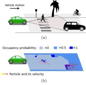
ward fully-autonomous car. For realizing the features cited above, various technologies of sensors (stereo-vision, radar, Light Detection and Ranging (LIDAR), etc) are embedded on IVs for observing the surrounding environment. Regard-ing the sensor readRegard-ings, the ADAS dispose a block called perception system, for building a computational model of the surrounding that the vehicle can interpret. For this purpose, the Hybrid Sampling Bayesian Occupancy Filter (HSBOF) [7] is a perception algorithm that builds a grid-based model of the environment. As shown in figure 1, the HSBOF maps the surroundings into a fixed size 2-dimension (2D) spatial grid divided into regular spatial cells. For each cell, the HSBOF computes the occupancy probability, that is, the probability that the cell is occupied, and estimates the ve-locity of the content of the cell. The nature of the obstacle occupying the cell does not matter. The occupancy proba-bility is then updated according to new sensor readings. The output grid is called occupancy grid.

(a)

(b)

Figure 1: Principle of HSBOF. (a) the surrounding environment is mapped into a 2D grid. (b) Occu-pancy Grid and Velocity estimation

The grid-representation of the internal data implies that HSBOF is a highly data-parallel problem where the same set of operations is applied to each cell. A rectangular grid with given width and height, and squared cells, is used. The cell sides define the resolution of the grid. Thus, in one

hand, a lower resolution implies a more accurate estimation of the spatial position of the obstacles. In the other hand, when the resolution decreases, the number of cells increases, and the number of computation follows on. Consequently, to be embedded on IVs, HSBOF should run on a hardware that provides enough computation performance to get an accurate result.

Choosing the right hardware architecture for integrating HSBOF into IVs remains a challenge. First, the hardware has to provide enough computational performance. Second, its purchase cost has to be low for being adopted for the mass production in the automotive industrie. Third, the limited energy resource on vehicle imposes that the hardware has to consume an electrical power as low as possible. Currently, the HSBOF is implemented on a Graphics Processing Unit (GPU) from NVIDIA [7], using the Compute Unified De-vice Architecture (CUDA) as a programming model. While providing a high computational performance, the GPUs con-sume a lot of energy. High-end GPUs concon-sume easily a hun-dreds of watts, which represents a significant charge for the electrical batteries on IVs. Moreover, the GPUs are too ex-pensive for the embedded market. They were not designed for an embedded use. On the software point of view, CUDA belongs to NVIDIA and is implemented only on their GPUs. Thus, the question arises: which hardware/software architec-ture can be used for replacing the GPU/CUDA architecarchitec-ture? Concerning the hardware architecture, the first existing solution is the multi-core Central Processing Unit (CPUs) which were already used for executing perception systems in [4, 8]. Embedded multi-core CPUs, mainly designed by ARM, outperform on generic tasks. But with their dual, quad or octa-core, they are optimized for multi-threading, thus for task-parallel problems, not for data-parallel algo-rithms. Further more, embedded CPUs do not provide enough computational performance for executing highly data-parallel algorithms such as the HSBOF.

The second solution is the embedded Multi-Processor Sys-tem on Chip (MPSoCs) which are initially designed for em-bedded uses and have more computational cores than CPUs but less than those of GPUs. The advent of MPSoCs relates the convergence of the hardware toward a more heteroge-neous architecture composed of a host and one or more hard-ware accelerators. The host is generally made of a multi-core CPU. Existing MPSoCs are generally equipped with one of the following hardware accelerator: 1) an embedded GPU as in the processor Tegra K1 from NVIDIA, 2) one or more Digital Signal Processors (DSPs) as the in the Keystone II designed by Texas Instrument, 3) a many-core acceler-ator as in the Parallela board or the MPPA many-core from Kalray. The architecture of these accelerators are very dif-ferent. They all might be an alternative to the GPU but in the present work, we focus first on many-core architecture. On a software point of view, we need a parallel programming model which is, first, adapted to the data-parallel nature of HSBOF. Second, the programming model must allow the developer to take advantage of the parallelism in the many-core architecture and the heterogeneity of the MPSoC. The OpenCL standard [1], a priori meets the two criterion. It was specifically designed for programming task-parallel and data-parallel algorithms on heterogeneous systems.

In this paper, we present a case-study on the feasibility of the utilization of the couple many-core/OpenCL as a hard-ware/software architecture for replacing the GPU/CUDA.

Through our OpenCL implementation and experiments, we prove that the many-core disposes enough computational performance for producing an occupancy grid in a reason-able time while consuming a lesser energy compared to GPU. On our testing hardware, the computation time of one iter-ation of HSBOF can reach 168ms, that is, about the double of the computation time on GPU. However, the many-core accelerator consumes only 1W , which is 40 times less than the GPU.

The current paper is organized as follow. Section 2 ex-plains the principle of the perception algorithm HSBOF. Section 3 presents the hardware/software platform. The OpenCL implementation is detailed in section 4. Experi-mental results are presented and discussed in section 5. Fi-nally, Section 6 concludes the paper.

2.

THE PERCEPTION ALGORITHM

As shown in figure 1, the Hybrid Sampling Bayesian Oc-cupancy Filter (HSBOF) [7] models the environment as a 2D grid. The algorithm produces an occupancy grid. It estimates also the velocity of the occupant of each cell and computes another grid called static grid. In contrast to the occupancy grid, the static grid contains the probability that each cell is occupied by a static obstacle (a non-moving ob-stacle). HSBOF is a mix of a classic Bayesian grid-filtering and a particle-based approach. According to the state of each cell at time tn−1, that is, its occupancy probability,

static probability and estimated velocity, the algorithm pre-dicts the state at time tn, and updates this prediction with

new sensor observations. By assuming that cell states are in-dependent, the HSBOF can be seen as a data-parallel prob-lem because the same set of operations are independently applied on each cell.

Concerning the velocity estimation, an obstacle can have theoretically an infinite possibility of velocity. Because, the algorithm cannot consider all of these possibilities, it focuses only on some samples of velocity. A set of particles rep-resents the samples. Actually, a particle is interpreted as a fictive point having a spatial coordinates, a velocity and a weight. The particle weight represents the probability that the speed of the content of the cell in which the particle is located, is actually the speed of the particle. We assume that unoccupied cells and cells occupied by static obstacles have a null velocity. Thus, HSBOF propagates the particles so that they follow the motion of the content of cells occu-pied by dynamic obstacles. For the sake of simplicity, these cells are called ”dynamic cells”.

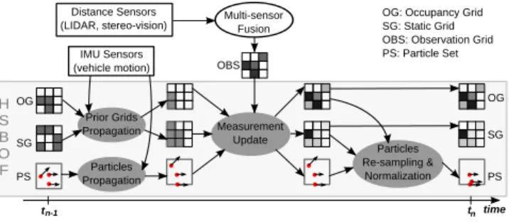
H S B O F OG SG PS Prior Grids Propagation Particles Propagation Measurement Update Particles Re-sampling & Normalization Multi-sensor Fusion OG SG PS OBS time OG: Occupancy Grid SG: Static Grid OBS: Observation Grid PS: Particle Set Distance Sensors (LIDAR, stereo-vision) IMU Sensors (vehicle motion) tn-1 tn

Figure 2: Overview of the HSOF algorithm Figure 2 presents an overview of the main steps of HS-BOF. The static grid, the occupancy grid, a set of particles

at time tn−1and an observation gird build from sensor

mea-surements constitute the inputs. The outputs are composed by the same elements but at time tn. The static grid and

the occupancy grid at time tn−1 are called prior grids. The

algorithm follows a particle filter approach with three steps: 1) particles and prior propagation, 2) measurement update, and 3) particles re-sampling and normalization.

2.1

Particles and prior propagation

The motion of the ego-vehicle is tracked by Inertial Mea-surement Unit (IMU) sensors such as odometer, accelerome-ter and gyroscopes. The 2D grid on figure 1(a) is fixed in the front of the vehicle. When the ego-vehicle moves, the grid is also displaced. The priors have then to be propagated in the new spatial placement of the 2D grid. The priors prop-agation is shown on figure 3(a). The prior grid at time tnis

computed by applying a linear interpolation on the cells in the occupancy and static grids tn−1. Concerning the

parti-cles, they are propagated in the space according to a motion model. Their position are updated depending on their speed and the duration ∆t = (tn− tn−1) (see figure 3(b)).

Vehicle M otion Occ/Static grid at time tn-1 tn Prior grid at time World x y (a) Particles set at time tn-1 tn Particles set at time Vehicle M otion World x y (b)

Figure 3: (a) Prior grids propagation. (b) Particles propagation.

2.2

Measurement update

As explained on figure 2, the measurement update is for updating the occupancy probability, and the static prob-ability of each cell regarding the sensor observation. The weight of every particles in a given cell is also updated ac-cording to the static and occupancy probability of that cell. It applies a bayesian program which mathematical formula-tion is detailed in [7]. We notice that an addiformula-tional process called multi-sensor fusion processes the sensor readings and produces an observation grid. In simple words, the ob-servation grid is closely related to the probability that each cell is occupied, regarding to the sensor readings [2].

2.3

Particle re-sampling and normalization

A re-sampling process is necessary for avoiding particles degeneracy, that is, for cell having particles, all but one par-ticle will have negligible weight. A new set of parpar-ticles is sampled from the previous set regarding their weights [7]. This step changes the local number of particles per cell by affecting more particles to dynamic cells. Particles with high weights are duplicated while particles with low weights are removed. After re-sampling, particle weights are normalized so that their sum per cell equals to 1.

3.

HW/SW PLATFORM

As HSBOF computes and updates probabilities for each cell of the 2D grid, an instinctive way to store the probabili-ties is using arrays of floating points. For an implementation on a parallel platform, the arrays can be seen as shared re-sources among the processing cores. OpenCL [1] is an appro-priate standard for a parallel-shared memory programming model. OpenCL can be mapped on many-core SoCs. It was initially designed for parallel heterogeneous systems.

3.1

OpenCL platform model on many-core

The OpenCL platform model is devided into two parts : one host as a central processing unit (CPU) and one or many compute devices which are hardware accelerator. A compute device is composed by one or many Compute Units. The lat-ter is further divided into one or more processing elements (PE). Figure 4 shows an example of how the OpenCL plat-form is mapped on a many-core SoCs. The compute device is the actual many-core platform while the host is mapped to more general CPUs such as an ARM processors and runs traditional operating system (linux, android, etc.).

L2 H O S T Many-core Processing Element Compute Device Compute Unit

Figure 4: OpenCL platform model on many-core

SoC.

3.2

OpenCL memory and execution model

In the OpenCL execution model, the parallelized tasks ex-ecuted on compute devices are called kernels. An instance of a kernel is called work-item. Work-items are grouped within a work-group. A set of work-groups forms an NDRange. Consequently, kernels are executed accross an NDRange. A work-group is affected to a compute unit. Then, processing elements execute the work-items.

Figure 5: OpenCL Memory model [1]

in a compute device. Each PE has its own private and fast memory. Local memories are shared memory for compute units. Work-items in a work-group can share data through local memories. Global and constant memory are accessible by all work-items. They are slower and might be cached depending on the capabilities of the device. For improv-ing the memory bandwidth, OpenCL exposes the control of DMA blocks to the developer if they are available on the hardware.

4.

IMPLEMENTATION

For implementing the HSBOF on an embedded many-core SoC using OpenCL, four points are interesting to be detailed: 1) how to schedule the different steps of the al-gorithm, 2) how to utilize the memory model in order to improve the performance, 3) how to map them on on the OpenCL platform, 4) what NDRange size is suitable for the algorithm.

4.1

Tasks and Scheduling

The HSBOF and the multi-sensor fusion form our per-ception system. The overall can be divided into five main tasks : 1) Particles Propagation , 2) Priors Propagation, 3) Measurement Update, 4) Particles Re-sampling and Nor-malization and 5) Multi-sensor Fusion. After that, the re-sampling and the particles normalization are separated into two subtasks. Furthermore, the particles propagation con-tains also two subtasks : Propagate Particles and Reorder Particles. The first actually propagates the particles as de-scribed above. The second subtask is explained in section 4.3.

Two scheduling policies can be explored. First, a sequen-tial scheduling policy executes all tasks sequensequen-tially, one af-ter the other. An executed task can then utilize all the computing resource and memory available on the hardware. It allows us to tune tasks separately and improve their indi-vidual performance. Second, by exploiting the input/output dependency on figure 6, a parallel scheduling policy can be implemented for reducing the overall execution time.

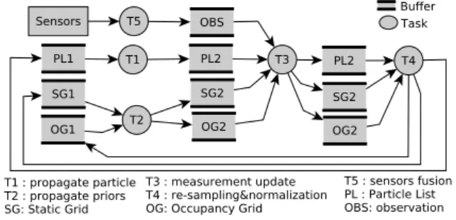
Figure 6: Perception system task level parallelism and buffers read/write

4.2

Memory mapping

As shown on figure 6, the occupancy prior at time tn−1

and the occupancy grid at tnare stored in two buffers OG1/2.

The buffers SG1/2 are for storing the static prior and the newly computed static grid. The particles are placed into the buffer P L1/2. All these buffers are shared resources for

work-items. They should be stored in global or local mem-ory. However, due to the limited size of local memories, the global memory is preferred. The data locality is prepon-derant in OpenCL. For a fast access, data processed by PEs should be placed in private or local memories.

For improving the memory bandwidth, OpenCL provides special Application Programming Interfaces (APIs) for han-dling DMA. It is used for transferring a block of data be-tween the local and global memory. Moreover, it allows us to use a double buffering technique for improving the mem-ory bandwidth. While working on a first rectangular portion of an input/output grid placed in the local memory, a sec-ond portion is DMA-transfered from global into a reserved region of the local memory. It will be processed when the first portion is treated. The double-buffering technique with DMA transfer allows to overlap the computations and the memory access.

4.3

Platform mapping

Two main computation resources can be used on the OpenCL platform: the host and the compute device. All tasks and subtasks of HSBOF can be parallelized except the subtask Reorder Particles. The smallest or ”native” data granularity is a cell for grid-related tasks, and a particle for particle-related tasks. For the sake of performance, the computa-tion should be aggregated by matching the number of work-items to the number of PEs. Thus, the granularity of a work-item becomes coarser in the sense that it has now to process several ”native” data instead of only one.

Concerning the subtask Reorder Particles, for a given cell, the weight of every particles in that cell is updated in the Measurement Update step. The subtask Reorder Particles arranges the particle buffer P L2 so that the particles in the same cell are stored in contiguous memory. In this way, the particles can be DMA-transfered and processed on the local memories. The subtask Reorder Particles uses a sequential sort algorithm. It can be then implemented on the OpenCL host which is more optimized for sequential operations.

5.

EXPERIMENTAL RESULTS

The HSBOF has two global parameters : the grid reso-lution and the number of particles. For a given width and length of the 2D grid, the value of the resolution determines the number of cells. We realized experiments and measured performance by changing the values of the algorithm param-eters.

5.1

Experimental Setup

For a testing purpose, we implemented the HSBOF on an off-the-shelf embedded low-power MPSoC [6], composed of a host and a many-core compute device. A dual core ARM Cortex A9 running at 800MHz serves as a host. The com-pute device comprises four comcom-pute units. A comcom-pute unit features a block made of 16 processing elements (PEs) and a 256 KBytes shared L1 and a DMA block. The L1 mem-ory serves as the private and local memories for the PEs. For the sake of performance, the number of work-items in a work-group is limited to 16. The compute device disposes a fast global memory L2 of 1MBytes. It can also share data with the host through a 1GByte of DRAM. But the later is slower compared to the L2. Data on real scenarios from eight LIDARs and IMUs are stored in files and are used as input for the multi-sensor fusion. These data were collected

through the experiments realized in [7].

5.2

Performance measurement and validation

For quantifying the performance, two criterion are ana-lyzed: the computation time and the power consumption. The overall computation time consists of the average dura-tion of the execudura-tion of one iteradura-tion of the algorithm. We also measure the computation time of individual tasks. The power consumption concerns only the compute device (the many-core). It is deduced from voltage and current mea-surements on oscilloscope.

Validation: An implementation of HSBOF on an GPU from NVIDIA already exists [7] and will serve as reference. Between the occupancy grids produced by the GPU and the many-core, the average relative error of the occupancy probabilities is 2%. It can be explained by the difference in the design of the two hardware and the random nature of the particle filter. This low difference confirms that the many-core implementation behaves as expected.

5.3

Overall Computation Time

For a 30m×50m grid, we tested two resolutions : 0.1m and 0.2m, which respectively correspond to two cell numbers : 150000 and 375000. The table 1 shows the overall computa-tion time regarding the particle number and the cell number. The size of the global memory on the compute device limits the maximum of particle number to 19000. By changing the algorithm parameters, the overall computation time on the many-core varies between 487ms and 168ms which is in the state of the art [5].

Part. Num. Res.(m) Cell Num. Comp. Time.(ms) 19000 0.1 150000 487 19000 0.2 37500 325 10000 0.1 150000 387 10000 0.2 37500 168

Table 1: Overall Computation Time

5.4

Individual Tasks Performance

This paragraph presents an analysis of the effect of the HSBOF parameters and OpenCL parameters on the indi-vidual performance of each task.

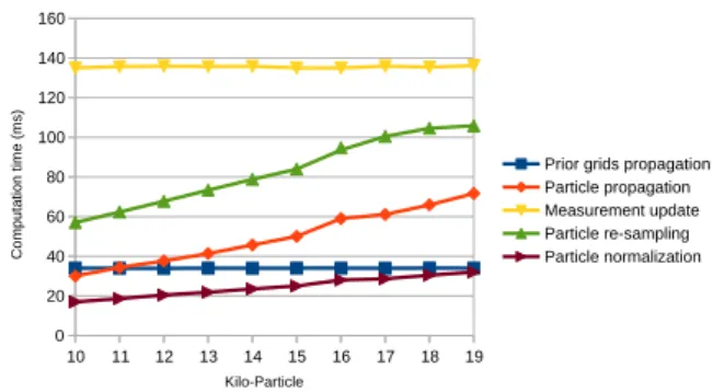
Number of particles: For a 30m × 50m grid, the fig-ure 7 plots the tasks computation time when changing the number of particles. The Prior Propagation does not de-pend on particles, its computation time remains constant. We notice the same behavior for the Measurement Update. In opposite, the duration of the Re-sampling and Particles Propagation increases linearly with the number of particles. This behavior is normal because these tasks process only particles.

Number of cells: While the grid width and length re-main constant (30m × 50m), the number of cell changes depending on the resolution of the grid. On figure 8, the number of particles equals to 19000. When increasing the resolution, the computation time of the Priors Propagation, the Measurement Update and the Multi-sensor Fusion are subject to exponential decay. Indeed, they apply the same set of operations for each cell, which make their duration very sensitive to the cell number. Table ?? and figure 8 shows that passing from a resolution of 0.1m to 0.2m re-duces the overall computation time by more than 150ms. Besides, we notice that the Particle Propagation performs

10 11 12 13 14 15 16 17 18 19 0 20 40 60 80 100 120 140 160

Prior grids propagation Particle propagation Measurement update Particle re-sampling Particle normalization Kilo-Particle Co m pu ta tion tim e (m s)

Figure 7: Computation time vs number of particles

slower when the resolution increases. Actually, the paral-lel subtask Propagate Particles processes only particles and does not depend on cell number. However, the sequential subtask Reorder Particles becomes slower due to a collat-eral effect of the Re-sampling process.

10 15 20 25 30 35 40 50 55 60 65 70 75 0 20 40 60 80 100 120 140 160

Prior grids propagation Particle propagation Measurement update Particle re-sampling Particle normalization Multi-sensor fusion

Length of the sides of the cells (cm)

Co m pu ta tion tim e( m s)

Figure 8: Computation time vs grid resolution Scalability: Scaling an application on OpenCL implies changing the number of the running work-items. We chose the Measurement update to prove the effect of scalability since it process a high number of input/outputs and has a higher computation time. The figure 9 shows that the Mea-surement update scales in a sub-linear fashion. A speedup gain is observed with a number of work-item between 1 and 14. Beyond this number, using more work-items does not bring any improvement. This result can be exploited to min-imize the energy consumption. For instance, in our testing hardware, the many-core disposes a hardware component that can be software programmed to reduce the clock fre-quency of the unused compute units. A fine grained energy management can be then implemented.

1 2 4 6 8 10 12 14 16 20

1 1,5 2 2,5

Meas. Up. Speedup

Number of work-items S pe ed up Linear Speedup Wasted Power

Figure 9: Measurement update speedup DMA transfer size: The probability distribution pro-cessed by the algorithm are stored in buffers of floating point.

For a 30m × 50m grid with a resolution of 0.1m and 19000 particles, the buffers consumes about 6MBytes of memory. In our implementation on the testing hardware, a particle buffer is placed in the L2 global memory, the other buffers are stored in the DRAM which is slower. The memory band-width can be improved by using a the double buffering tech-nique with a DMA transfer as explained above. We notice in our tests that the more data are coalesced into a DMA block, the less the computation time is. On our testing hard-ware, a speedup of ×7 can be achieved by choosing the right size of the DMA block transfer.

5.5

Discussions

An implementation of HSBOF in CUDA already exists [7]. We run it on a GPU Quadro FX 1700 from NVIDIA for a comparison to our many-core/OpenCL implementation. The results are shown on figure 10. By increasing the reso-lution from 0.1m to 0.2m, the overall computation time on the many-core is significantly reduced. By also decreasing the number of particles to 10000, the many-core performs at 168ms while 90ms for the GPU. In the three configurations, it is clear that the GPU beats the many-core concerning the computation time (see figure 10(b)).

However, as shown on figure 10(a) ,the GPU consumes typically 40W , while the many-core power consumption is less than 1W (actually between 883mW and 967mW ). The many-core consumes then 40 times less power than the GPU. GPU Many-Core 0 5 10 15 20 25 30 35 40 45 Power C o n su mt ion (W) 1 (a) 0 100 200 300 400 500 C o m pu ta tio n time( ms ) Many Core G P U G_P U G P U Particles 19000 Cells Sides 0.1m Particles 19000 Cells Sides 0.2m Particles 10000 Cells Sides 0.2m Many

Core ManyCore

(b)

Figure 10: Many-core vs GPU. (a) Power Consump-tion. (b) Computation Time

Is the result promising for a future integration into IVs? The choice of the value of the particle number and the grid resolution depends on the observed environment. Resolutions between 0.1m and 0.2m were tested in [7][3]. Furthermore, the particle number depends also on the num-ber of cells, thus, on the resolution. While currently, we do not dispose yet a formal method for estimating the correct number of particles, we assume that fewer cells implies fewer particles. Thus, the algorithm parameters can be adapted to the street scenario. For instance, in cities, the obstacles are numerous and their nature are diversified. It can vary from a vehicle to an animal. Consequently, a lower resolution with a high number of particles is then needed. However, on high-way, obstacles are mainly vehicles running at high speed. A higher resolution with few particles are then acceptable.

We deduce then that the performances (computation time and power consumption) we get on the many-core are

promis-ing. On the one hand, even if the GPU beats the test-ing hardware in term of computation time, the many-core performs an interesting computation time of 168ms by finding a trade-off on the algorithm parameters to get val-ues that can be adapted to certain scenarios. On the other hand, the power consumption on the many-core is 40 times lower than on the GPU. The result in the second line on table 1 represents an example of trade-off between the number of particles (19000) and the resolution (0.2m). The power consumption remains low (less than 1W ) and the computation time lasts 325ms which is still in the state of the art navigation requirements according to [5].

6.

CONCLUSION

The HSBOF needs a high computational performance to be executed in a reasonable duration. It is currently imple-mented in CUDA on a NVIDIA GPU that is power consum-ing. In this paper, we proved that, the couple embedded many-core/OpenCL is a feasible hardware/software archi-tecture for replacing the couple GPU/CUDA. The experi-mental results are promising. They were validated by a low average relative error compared to the results produced by the GPU. While consuming a lesser power, the many-core can produce an occupancy grid within a reasonable time. On our testing hardware, the many-core consumes less than 1W which is 40 times less power consmption than the GPU. Though, the many-core can output an occupancy grid every 168ms. These results are obtained by tuning the implemen-tation parameters provided by OpenCL: the mapping of the algorithm on the available computing resources, the scalabil-ity, the data locality and the DMA for improving the mem-ory bandwidth. We conclude that the many-core/OpenCL is a promising hardware/software architecture for integrating HSBOF into intelligent vehicles.

7.

REFERENCES

[1] The open standard for parallel programming of heterogeneous systems. www.khronos.org/opencl. [2] J. D. Adarve, M. Perrollaz, A. Makris, and C. Laugier.

Computing Occupancy Grids from Multiple Sensors using Linear Opinion Pools. In IEEE ICRA, 2012.

[3] Q. Baig, M. Perrollaz, and C. Laugier. A robust motion detection technique for dynamic environment monitoring: A framework for grid-based monitoring of the dynamic environment. Robotics Automation Magazine, IEEE, 2014. [4] C. Cou´e, C. Pradalier, C. Laugier, T. Fraichard, and

P. Bessiere. Bayesian Occupancy Filtering for Multitarget Tracking: an Automotive Application. International Journal of Robotics Research, 2006.

[5] D. Held, J. Levinson, and S. Thrun. Precision tracking with sparse 3d and dense color 2d data. In ICRA 2013.

[6] Melpignano et al. Platform 2012, a many-core computing accelerator for embedded socs: performance evaluation of visual analytics applications. In DAC 2012.

[7] A. Negre, L. Rummelhard, and C. Laugier. Hybrid sampling bayesian occupancy filter. In Intelligent Vehicles Symposium Proceedings, 2014 IEEE.

[8] T. Weiss et al. Robust driving path detection in urban and highway scenarios using a laser scanner and online occupancy grids. In Intelligent Vehicles Symposium, 2007 IEEE.