HAL Id: cea-02339325
https://hal-cea.archives-ouvertes.fr/cea-02339325
Submitted on 14 Dec 2019HAL is a multi-disciplinary open access
archive for the deposit and dissemination of sci-entific research documents, whether they are pub-lished or not. The documents may come from teaching and research institutions in France or abroad, or from public or private research centers.
L’archive ouverte pluridisciplinaire HAL, est destinée au dépôt et à la diffusion de documents scientifiques de niveau recherche, publiés ou non, émanant des établissements d’enseignement et de recherche français ou étrangers, des laboratoires publics ou privés.
thermalhydraulic codes with 3d-pressure vessel
modelling
D. Bestion
To cite this version:
D. Bestion. Specific requirements for bepu methods using system thermalhydraulic codes with 3d-pressure vessel modelling. BEPU-2018, May 2018, Lucca, Italy. �cea-02339325�
SPECIFIC REQUIREMENTS FOR BEPU METHODS USING SYSTEM THERMALHYDRAULIC CODES WITH 3D-PRESSURE VESSEL MODELLING
D. Bestion,
Commissariat à l’Energie Atomique CEA-GRENOBLE, DEN-DM2S-STMF, 17 Rue des Martyrs, GRENOBLE Cedex, FRANCE
ABSTRACT
The 3D modules of system thermalhydraulic codes were first used for transient analysis with a very coarse nodalization including only a few hundreds of meshes in the whole pressure vessel. Today the increased computer power allows 3D simulations with a much finer nodalization for many new transients. A core modelling with one mesh per assembly may become a standard practice in near future. This allows to look at much finer multi-dimensional physical processes and may provide a better accuracy of predictions. Specific requirements are necessary for such finer simulations. First, a more detailed PIRT exercise should identify dominant phenomena at a smaller scale than for previous nodalizations. Based on porous body 3D equations, one can identify a list of phenomena to model and to validate on specific separate effect tests. This includes the turbulent diffusion of heat and momentum, the void dispersion, and the heat and momentum dispersion due to space averaging. In addition, 3D wall friction and interfacial friction tensors have to be developed and validated for non-isotropic media like core rod bundles. An order of magnitude analysis may allow to neglect some of these processes or simplify some models, depending on the sub-component (core, lower plenum, annular downcomer, upper plenum) and depending on the physical situation encountered in accidental transients. Attention will be drawn on LOCA situations in PWRs and on the core component of the Pressure Vessel. The degree of completeness of the physical modelling and of the related validation is evaluated. The impact of numerical errors and of the node size is discussed. Directions are given for future BEPU methods applied to a core modelling with one mesh per assembly by considering a multi-scale validation of the dominant 3D processes.
1. INTRODUCTION
System thermalhydraulic codes have 3D models in porous medium approach which were initially devoted to the prediction of very large scale 3D effects during LBLOCAS and which were validated on the data of the 2D-3D experimental program performed in UPTF, SCTF and CCTF facilities. The application of BEPU methods using system codes for licensing used first rather coarse reactor nodalization with 0-D and 1D modules or components to allow many code runs for uncertainty propagation while keeping a reasonable total CPU time. 3D modules were used for transient analysis with a very coarse nodalization including only a few hundreds of meshes in the whole pressure vessel. Today the increased computer power allows 3D simulations with a much
finer nodalization for many new transients. A core modelling with one mesh per assembly may become a standard practice in near future with the CATHARE code for many accidental transient simulations including LOCAs. This allows to look at much finer multi-D physical processes and may provide a better accuracy of predictions. Specific requirements are necessary for such finer simulations. First, a more detailed PIRT exercise is needed to identify dominant phenomena at a smaller scale than for previous nodalizations. Based on porous body 3D equations, one can identify a list of new phenomena (compared to 1D approach) to model and to validate on specific separate effect tests. An order of magnitude analysis allows to neglect some of these processes or simplify some models, depending on the sub-component (core, lower plenum, annular downcomer, upper plenum) and depending on the physical situation encountered in accidental transients. Attention will be drawn on LOCA situations in PWRs and on the core component of the Pressure Vessel. The degree of completeness of the physical modelling and of the related validation will be evaluated. The impact of numerical errors and of the node size is discussed. Recommendations are made for future BEPU methods applied to a core modelling with one mesh per assembly. A new approach called “multiscale validation” is proposed.
2. EVOLUTION OF PWR PRESSURE VESSEL MODELLING
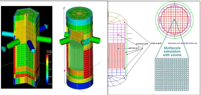
The current generation of industrial system codes (CATHARE, RELAP-5, TRACE, SPACE, ATHLET) can model the pressure vessel either by assembling 0D and 1D models or with 3D pressure vessels (PV) which started to be developed in the 80s. The core was initially modelled as a 1D component, or by parallel 1D modules possibly with crossflows to take into account in some way the radial transfers due to the radial power profile. When using a full 3D PV modelling, the initial nodalization was very coarse due to high CPU cost. A typical 3D modelling in cylindrical coordinates included about 20 meshes in vertical direction with 10 to 12 in the core, 5 radial meshes and 6 or 8 azimuthal meshes respectively for 3-loop and 4-loop reactors. The core axial meshing was far from mesh convergence since about 40 axial meshes are necessary to obtain a convergence of a Figure of Merit (FoM) like the peak clad temperature (PCT) with a tolerance of a few degrees in LBLOCA conditions. Using 11 meshes in axial meshing could induce a PCT error of 20 to 30 K when simulating Reflooding tests with the CATHARE code. However, this was not a big issue since the uncertainty on PCT is estimated to at least +/- 150 K. The numerical error could be hidden by the uncertainty due to initial and boundary conditions, physical properties and closure laws. The continuous increase of computer power allows much finer nodalizations as illustrated in Figure 1 in order to reduce both numerical errors and physical model uncertainties. Developments of the CATHARE code 3D module make it possible to combining various sub-components using either cartesian, cylindrical or elliptical frames of reference depending on the local geometry as shown in Figure 1. One may also imagine local mesh refinements in one or a few fuels assemblies which would be treated by channel analysis model, i.e. with one raw of meshes for each sub-channel.
On the left (Figure 1) one can see an old nodalization of a 3 loop reactor with a cylindrical coordinate and 5 radial, 6 azimutal and 21 vertical meshes for a total of 630 meshes only (198 meshes in the core). In the centre (see Prea et al., 2017,[1]) , one can see a cylindrical system of coordinates in all parts except the core which is modelled in a cartersian frame of reference and one column of meshes per assembly. There is one radial mesh in the downcomer, one for the core baffle, and 5 radial meshes in lower plenum, upper plenum and upper head. This nodalization is clearly much finer in the core with about 6000 meshes. This paper considers such advanced
modelling and identifies the requirements for an acceptable BEPU method application with a good VVUQ (validation verification and uncertainty quantification).
Figure 1: Illustration of the nodalization of a PWR pressure vessel using a 3D module. On the left an old coarse nodalization; in the centre a recent finer nodalization particularly in the core. On the right, Pressure Vessel with Cartesian, cylindrical and elliptical coordinates and with a possible local zoom with sub-channel analysis in one or a few assemblies.
3. REVISITING PIRT AND BEPU APPROACH FOR A 3D MODELLING 3.1 The various steps of a BEPU approach
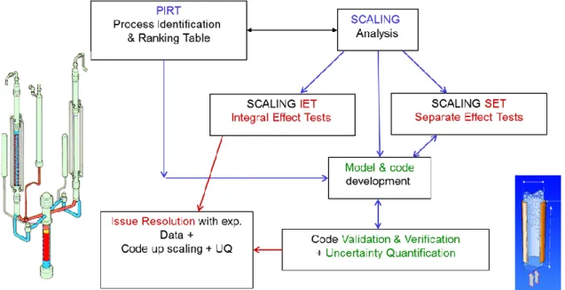
A general BEPU method is illustrated in the Figure 2 with the various step. BEPU includes a PIRT analysis, a scaling analysis, the selection of scaled Integral Effect Tests (IET) or Combined effect tests (CET) and Separate Effect Tests, the selection of a numerical simulation tool, the Verification and Validation of the tool, the code application to the safety issue of interest and the uncertainty quantification (UQ) of code prediction.
PIRT: Phenomena identification analyzes and subdivides a complex system thermal-hydraulic
scenario into several simpler processes or phenomena. During the physical analysis, it is useful to discern the dominant parameters. The figures of Merit (FoMs) are identified as well as all dominant processes and parameters which have an influence on them. For LOCAs, the main FoM is the PCT. Ranking establishes a hierarchy between processes with regards to their influence on the FoMs. PIRT can start by expert assessment, analysis of some experiments, and can then iterate by using sensitivity studies with simulation tools.
Scaling analysis: the scaling analysis is an important step to build a methodology to solve an issue
by using both scaled experiments and numerical tools able to correctly reproduce all identified dominant phenomena and extrapolate to the reactor scale. It includes the scaling of IET and SET experiments showing to what extent they can be sufficiently representative of the real process in a reactor. Another step is to identify the requirements for the numerical simulation tool so that it can
model all dominant processes and can be applied with sufficient confidence to the real process, demonstrating its scalability.
Usual scaling methods such as H2TS (“Hierarchical Two Tiered Scaling”) have two steps: a top - down, T-D, and a bottom - up (B-U). The T-D step uses non-dimensional form of mass (M), energy (E) and momentum (MM) conservation equations written at the system level to establish the scaling hierarchy i.e. what phenomena have priority in order to be scaled (e.g in an IET), and to identify what phenomena must be included in the bottom-up analysis. The B-U step continues the analysis at the component or at the process level to scale SETs and both steps give requirements for the physical modelling in the simulation tool and of the validation of the tool. The scaling analysis is based on the PIRT but it can also help the PIRT by helping in the ranking of phenomena.
Figure 2 – The various steps of a BEPU approach applied to a PWR safety issue.
Verification Validation and Uncertainty Quantification (VVUQ)
V&V activities are dealing with numerical and physical assessment.
Verification evaluates the software correctness and numerical accuracy of the solution to a given physical model defined by a set of equations. Verification covers: Equations implementation, calculation of convergence rate for code and solution verification
Validation of a code evaluates physical models of the code based on comparisons between simulations and experimental data. It may be used also to quantify the accuracy or to determine the uncertainty of closure laws. A validation matrix is a set of experimental tests for an extensive and systematic validation of a code. It usually includes SETs and IETs with possible CETs. Validation matrices are established for each accident scenario or for an ensemble of scenarios. They should cover all dominant processes identified during the PIRT + scaling analyses at system level and at component and process level. SET may be used to validate a closure relation independently from the others. IETs simulate the behavior of a complex system including the whole cooling circuit with all interactions between various flow and heat transfers processes occurring in various components. Combined effect tests (CETs) include usually a part of a whole system with several components and several coupled basic processes.
Uncertainties Quantification (UQ) starts by clearly identifying the various sources of uncertainties. Then uncertainty propagation methods may be used to determine the uncertainty of code results on a reactor transient simulation.
In the case of a 3D modelling of a reactor vessel or of a part of the vessel, the BEPU method should be revisited for:
1. PIRT revisiting and upgrading by identifying local 3D processes which can affect the FoMs 2. Perform the scaling analysis with order of magnitude evaluation of all local 3D processes 3. Complement the verification by analyzing the mesh and time step convergence conditions 4. Complement the validation matrix by specific tests on 3D local processes
3.2 Identifying local 3D processes
The system of equations used in porous-3D two-fluid model is the basis for identification of all relevant 3D processes. (see Chandesris et al., [2, 3] 2006, 2013):
𝜕𝜙𝛼𝑘𝜌𝑘 𝜕𝑡 + ∇. (𝜙𝛼𝑘𝜌𝑘𝑉𝑘) = 𝜙Γ𝑘 (1) 𝛼𝑘 𝜌𝑘(𝜕𝑉𝑘 𝜕𝑡 + 𝑉𝑘𝛻. 𝑉𝑘) +𝛼𝑘 𝛻𝑃 = (𝑝𝑖+ 𝑓𝑖 𝑇𝐷) 𝛻𝛼 𝑘∓ 𝜏𝑖+ 𝛼𝑘 𝜌𝑘𝑔 + 𝜏𝑤𝑘+𝜙1𝛻. (𝛼𝑘𝜌𝑘𝜏𝑘𝑡+𝑑) (2) 𝜕𝜙𝛼𝑘𝜌𝑘𝑒𝑘 𝜕𝑡 + ∇. (𝜙𝛼𝑘𝜌𝑘ℎ𝑘𝑉𝑘) = 𝜙q𝑘𝑖+ 𝑆𝑐q𝑤𝑘+ 𝜙Γ𝑘ℎ𝑘+ ∇. (𝛼𝑘𝑞𝑘𝑡+𝑑) (3) In these equations, 𝛼𝑘,𝜌𝑘,𝑉𝑘, 𝑒𝑘, ℎ𝑘 are the volume fraction, the density, the velocity, the internal energy and the enthalpy for the phase k, 𝜙 is the porosity, P the pressure, Γ𝑘 the interfacial mass exchange. 𝑝𝑖 and 𝑓𝑖𝑇𝐷are void dispersion terms due to space averaging of interfacial pressure forces, and time averaging of drag and added mass forces. They tend to homogenize void fraction. 𝜏𝑖 𝑖𝑠 the interfacial friction force, 𝜏𝑤𝑘the wall friction force, q𝑘𝑖, q𝑤𝑘 the interfacial and the wall to phase k heat transfer, 𝑆𝑐 the heating surface, 𝜏𝑘𝑡+𝑑the stress tensor which accounts for turbulent and dispersive effects, and 𝑞
𝑘𝑡+𝑑the turbulent and dispersive heat flux
Diffusion and dispersion terms
The momentum and energy dispersive and diffusive terms came out during the double (time and space) averaging process of the local convection terms:
< 𝑣𝑣̅̅̅ >𝑓=< 𝑣̅ >𝑓< 𝑣̅ >𝑓+< 𝑣′𝑣′̅̅̅̅̅ >𝑓+< 𝛿𝑣̅̅̅ 𝛿𝑣̅̅̅ >𝑓 (4) < 𝑣ℎ̅̅̅̅ >𝑓=< 𝑣̅ >𝑓< ℎ̅ >𝑓+< 𝑣̅̅̅̅̅ >′ℎ′ 𝑓 +< 𝛿𝑣̅̅̅ 𝛿ℎ̅̅̅ >𝑓 (5) 𝑥 ̅is the time average of the quantity x and x’ the deviation from this average:
< 𝑥 >𝑓 is the spatial average of the quantity x and 𝛿𝑥 the deviation from this average
The first rhs terms of equations (4) and (5) are the macroscopic convection of the mean velocity and enthalpy, the second rhs terms are the turbulent diffusion of momentum and energy, and the third rhs terms are momentum and energy dispersion terms (see Drouin et al, 2010, [4]).
Chandesris et al. [3] synthesized the present status of modelling and validation of these momentum and energy diffusion and dispersion terms for a PWR core available on option in the CATHARE code. The macroscopic Reynolds stress tensor is modelled following the microscopic eddy-diffusivity concept. The dispersive momentum term can be modelled in a similar way introducing a dispersive momentum coefficient.
𝜏𝑘𝑡+𝑑 = (𝜈
The macroscopic turbulent energy flux is modelled according to a generalized Fick’s law using a macroscopic turbulent thermal conductivity 𝛼𝑡𝑘𝜙. The dispersive heat flux can also be modelled using a first gradient hypothesis. Some models consider a thermal dispersive tensor 𝐷̿𝑑𝑘𝜙 to account for anisotropic geometry.
𝑞𝑘𝑡+𝑑= (𝛼𝑡𝑘𝜙𝐼 + 𝐷̿𝑑𝑘𝜙 ) 𝜙𝛻ℎ𝑘 (7) It was found in a core that dispersive fluxes usually dominate the macroscopic turbulent heat flux by two
or three order of magnitude and that turbulent fluxes also dominate molecular fluxes. It is also clear that spacer grids play a dominant role on dispersion effects and that dispersion is highly geometry-dependant. The presence of mixing vanes is playing a dominant role.
Models were obtained from 5x5 or at maximum 8x8 rod bundle data analysed at the sub-channel scale. In the same way as turbulent viscosity depends on the filter scale in single phase Large Eddy Simulation, diffusion-dispersion coefficients should depend on the spatial scale of the model. When a core is modelled with a porous-3D approach at a much larger scale (one assembly/ mesh, several assemblies/ mesh) than the sub-channel scale, the coefficients should be different. Today there is no general diffusion-dispersion model validated for every type of meshing and the applicability of current models to large scale nodalizations is not proved. There is a lack of data obtained in large dimension rod bundles with measurement of diffusion and dispersion effects. One can add that diffusion-dispersion of other scalar quantities such as boron concentration also needs validation.
Regarding the void dispersion term 𝑝𝑖 and 𝑓𝑖𝑇𝐷, which are related to spatial and temporal fluctuations of pressure and velocity at the interface, Valette (2011[5]) proposed some models for core geometry based on PSBT and BFBT benchmark data analysis at the sub-channel scale. However extension of the models and validation to larger scale modelling is also required.
3.3 Scaling analysis for local 3D processes
The geometry of the sub-components of a Pressure vessel have very different geometry and hydraulic scales. Therefore the relative weight of every single process in mass momentum an energy equations may be strongly dependent on the component. One may expect that components with small hydraulic diameters like the core will have a higher sensitivity to wall transfers than to diffusion and more open medium like the annular downcomer may be more sensitive to inertial and diffusive terms. Therefore the scaling analysis should be made for each component at each phase of each transient to determine the dominant 3D processes.
3.4 The 3D mesh and time step convergence issue
The use of 1D models of system codes require mesh convergence and time step convergence tests. Tolerance criteria depend on the situation of interest and on required accuracy of simulations. In many cases, the use of rather coarse meshes is acceptable although the first order upwind scheme induces a rather high numerical diffusion. The axial evolution of flow parameters are often dominated by convective terms and source terms due to wall and interfacial transfers, so that axial diffusion (molecular and turbulent) is negligible as well as numerical diffusion.
In a porous 3D model, the use of a double time and space integration over given space domains of a PV filters all mixing processes at a scale which depends on the mesh size. However such 3D approach may be considered as a juxtaposition of 0-D interconnected control volumes. This space integration is somewhat different from using a moving space filter associated to a homogenization of equations which actually results in 3D system of partial differential equations.
In our approach, all diffusive models have to be made dependent on the mesh size. The validation should also be made dependent on mesh size. No mesh convergence is required only time step
convergence is needed. However determining the model accuracy or uncertainty as a function of the space scale is a similar exercise as doing mesh convergence study in a homogenized space filtered model.
3.5 A specific PIRT and validation matrix for 3D local processes
One may synthesize the PIRT and scaling analyses specific to 3D approach to identify the validation needs using a table. An example is given in section 4.
Revisiting the PIRT for 3D modelling requires that 3D effects on all models are examined. There may be a geometrical effects on the flow regime and heat transfer regime and on all wall transfers, and interfacial transfers, compared to a 1D flow situation. In addition, in a 3D flow in a porous body, there may also be turbulent diffusion and dispersion of mass, momentum and energy due to time and space averaging. One may also identify specific 3D processes, such as gravity driven natural circulation, mixing layers, jets, wakes, flow curvature,…For each component of the vessel, each phase of each transient of interest, one evaluates the sensitivity of each process on the FoMs, the uncertainty on the existing models, the possible effects of specific geometrical details (spacer grids, flow restrictions, nozzles, …) on the process have to be identified. At last the validation data base are identified with processes which can be validated in a separate-effect way (best case), or validated more globally together with other sensitive processes, or even not validated at all (worst case). This analysis may be first done by expert judgement and then supported by sensitivity calculations. Defaults of the existing models may be identified which require further modelling efforts. Remaining validation needs are also identified.
4. 3D CORE MODELLING IN LOCAS
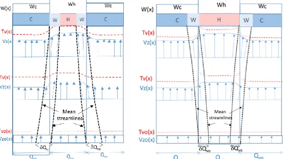
Although the flow is mainly vertical upwards in a core during LOCAs, rather important radial transfers exist which play a significant role on the PCT. Figure 3 illustrates typical SBLOCA situation during a core uncovering and LBLOCA during a reflooding. This comes mainly from observations and analysis of rather old experimental programs such as PERICLES 2D [6,7]. In both cases, the two-phase zone below quench fronts or below a swell level is well homogenized by a gravity driven recirculation which may also extend to the zone below the core. In such low velocity flow, the void dispersion force play a minor role in this mixing. This mixing is rather well predicted [6,7] without specific modelling efforts although the wall friction and interfacial friction for radial flow is not yet correctly addressed. A high uncertainty on these transverse frictions has not a big impact on PCT. In reflooding, the faster quenching in colder zones induces some liquid transfer to hot assembly just above its quench front (by simple gravity effects) which induces a better precooling and increases droplet entrainment in the dry zone of the hot assembly. This accelerates the quenching in hot zone and improves exchanges in dry zone by more steam cooling by droplets. In the swell level zone of a SBLOCA situation, gravity also homogenizes the level. In the dry zone with pure steam, gravity and density differences induce some significant chimney effect which improves the cooling of the hot assembly. It was found (Bestion et al 2015 [8], 2017, [9]) that crossflows may be from hot to cold assembly at lower pressure (e.g. P<1Mpa) since higher velocity creates more axial friction pressure losses and the crossflow is of diverging type from hot to cold. The transverse flow pressure losses are not well modelled nor validated and a high uncertainty is still required as long as no SET validation is available. Momentum and energy diffusion-dispersion may play some role in both situations. However previous work indicates that they may be of second order compared to crossflows. Recent calculations of core uncovering and
Reflooding PERICLES tests at the sub-channel scale using the validated diffusion and dispersion models of Chandesris et al (2013, [3] were done by Alku (2016, [10]) and have shown that the results were not very sensitive to any diffusion dispersion term. Moreover, it was found that all the mixing processes at the periphery of a hot assembly (momentum diffusion-dispersion, heat diffusion-dispersion and crossflows) create mixing layers which enlarge rather slowly so that one may expect that radial gradients within each assembly are never fully eliminated by mixing along the core height and that a high power assembly is probably mainly influenced by its direct neighbours.
Figure 3: Radial transfers due to power profile. A high power assembly with two lower power neighbours. Left: low P LBLOCA reflooding; Right high P SBLOCA core uncovering
One can identify three radial mixing processes between sub-channels or between assemblies: Radial momentum diffusion-dispersion
𝜏𝑧𝑥𝑑+𝑡~𝜇𝑡𝜕𝑉𝜕𝑥𝑧 homogenizes radially 𝑉𝑧 and creates a radial flow from high 𝑉𝑧 to lower 𝑉𝑧 Radial heat diffusion-dispersion
𝑞𝑥𝑑+𝑡~𝜆
𝑡𝜕𝑇𝜕𝑥 transfers heat from hot to cold assembly Crossflow by pressure radial differences
𝜕𝑃𝜕𝑥 = −𝐾𝑒𝑓𝑓𝑥
𝐿𝑥 𝜌
𝑉𝑥2
2 transfers fluid from from high 𝑉𝑧 to lower 𝑉𝑧 or from low 𝑉𝑧 to high 𝑉𝑧 transfers energy by convection from hot to cold assembly or from cold to hot assembly The current analysis of processes [8,9,10,11] is summarized in table 1. The chimney type crossflow has a favorable effect on PCT since the hottest assembly receives additional coolant flow and a colder coolant from neighbors. Diverging crossflow has a limited unfavorable effect since the hot assembly loses coolant but gives part of its energy to neighbors.
Table 1: PIRT analysis specific to a 3D approach for an uncovered core in a SBLOCA
3D EFFECTS IN AN UNCOVERD PWR CORE OF A SBLOCA
Process Sensitivity on FoM (H,M,L) Model Uncertainty (H, M, L) Geometry effect SET or global validation Flow regime identification H L in axial flow ? No
Interfacial friction H M ? Axial flow:OK
Radial flow : no
Wall friction & form loss M L in axial flow
H in radial flow spacers
Axial flow:OK
Radial flow : no
Void dispersion L H ? No
Interfacial H&M transfers L spacers No
Wall HT regime identification H L Axial flow:OK
Convection to liquid L L spacers Axial flow:OK
Nucleate boiling L M Axial flow:OK
CHF (DNB or dry-out) H L OK
Convection to vapor H L spacers Axial flow:OK
Heat diffusion-dispersion in liquid L M spacers PSBT
Heat diffusion-dispersion in steam L or M M spacers No Specific 3D processes Chimney effect Diverging crossflow M M M M Spacers spacers No PERICLES
5. VALIDATION PROGRAM FOR CORE
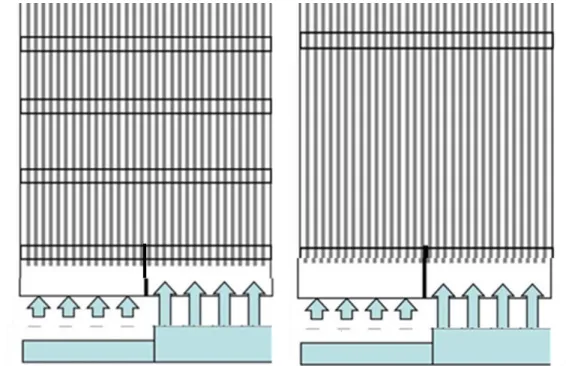
An experimental program has been built (see [11]) to investigate and model some of the 3D core processes and to allow separate effect validation for both sub-channel model and one per assembly model. This is a pure water or air-water test in 2 non-heated half assemblies. The METERO-vertical test facility allows an unbalanced feeding of both assemblies with either different tracer concentration, different velocities, different temperatures and different void fractions. It will be
possible to identify separately the effect of the rod bundle and of spacers by comparing the left and right configurations in Figure 5.
Figure 5: The METERO test section with possible unbalanced feeding. On right apcer grids are removed to investigate the influence of spacers
Various test series are planned to address the respective processes of interest. They are summarized in table 2. Such tests do not represent SBLOCA situations but include all processes of a SBLOCA situation. When sub-channel models and 1 mesh/per assembly models will be validated on such tests, more complex and representative SBLOCA situations may be simulated at sub-channel scale to obtain reference results for the 1 mesh/per assembly models. At last a global validation on existing large scale tests may be done using PERICLES data and some IET LOCA tests with radial power profiles such as some ROSA IV-LSTF tests.
Table 2: Test series in METERO test facility
Process Term of
equation
Test series Test conditions
Wall friction 𝜏⃗⃗⃗⃗⃗⃗ 𝑤𝑘 P losses in axial flow P losses in non-axial flow
Equal BC UV Momentum
diffusion-dispersion
tk Pressure losses with transverse flow UV-UT-equal 𝜕𝑃𝜕𝑧
With & without spacers Scalar turbulent
diffusion
tk
d
Mixing of a passive scalar in 1-phase flow EV-US No spacers
Scalar dispersion dk
Energy turbulent diffusion
tk Energy mixing in 1-phase flow UT No spacersEnergy dispersive tensor
dk
D Energy mixing in 1-phase flow UT
Two-phase wall friction And two-phase interfacial friction 𝜏𝑤𝑘 ⃗⃗⃗⃗⃗⃗ 𝜏𝑖 ⃗⃗
P losses and wall & interfacial friction in axial flow
P losses and wall & interfacial friction with transverse flows
P losses and wall & interfacial friction with buoyancy driven crossflows
EV-EX UV-EX UV-UX
Void dispersion TD
i
f
Void dispersion tests UV-UX- equal𝜕𝑃 𝜕𝑧
UV: unequal velocity; EV equal velocity; ES equal scalar (tracer concentration); US unequal scalar concentration; UT: unequal temperature; UX: unequal quality; equal 𝜕𝑃
𝜕𝑧 means that velocity
differences and temperature or quality difference are such that the axial P gradient are equal to avoid crossflows and to measure scalar or temperature or void diffusion-dispersion
6. SYNTHESIS AND CONCLUSION
The use of porous a 3D modelling of a PWR pressure vessel in a system code with more and more refined nodalization may provide more accurate and more reliable predictions but it requires some revisiting of the BEPU approach.
The PIRT exercise must be refined at the local level to identify dominant processes controlling local 3D effects. The diffusion and dispersion terms in momentum and energy equations and the void dispersion force require some attention. The 3D formulation of wall friction and interfacial friction must be considered as well as the 3D formulation of wall and interfacial heat and mass transfers. A scaling analysis and order of magnitude evaluations may help the ranking of processes. Such processes may have either a negligible or a significant effect on some FoM depending on the component (core, upper plenum, lower plenum, downcomer) and depending on the transient or even the phase the transient.
This ranking of processes for each component in each phase of each transient leads to identify the models which should be added or improved, which should be validated in a separate effect way and for which an uncertainty should be determined. This may need new experimental programs. A special attention must be paid to the impact of space resolution and to mesh convergence and time step convergence issues. Since space averaging is applied in the form of a space integration in a given domain of the reactor vessel and not as a space filtering with homogenization, mesh convergence is not required but the impact of the space scale on the physical processes should be modelled and the model uncertainty should be dependent on the space integration scale.
Local measurements are very difficult and very expensive in the extremely complex geometry of a reactor vessel. Therefore one can use a multi-scale validation strategy, with the following steps: Small size experiments (e.g. 5*5 rod bundle tests) are used for separate effect validation of
Small scale models (Sub-channel models) are used to simulate larger dimension problems (e.g. several assembly simulations)
Larger scale models (e.g. 1 mesh/assembly modelling) are validated against sub-channel model simulations.
A more global validation of the large scale model may be added with a large scale experiment with several assemblies(PERICLES, LSTF) even if there is lower density of instrumentation.
Looking at the core behaviour during LOCAS, previous work already identified the following dominant 3D processes which require a special attention:
Crossflow exist which may be gravity dominated (two-phase with low velocity below a swell level or below a quench front, or pure steam flow in uncovered zone at high pressure). They require a validation of transverse pressure losses and interfacial friction in non-axial flow.
Crossflow exist which may be friction dominated (two-phase with high velocity during LBLOCA blowdown, or pure steam flow in uncovered zone at low pressure in SBLOCAs and IBLOCAs). They require a validation of transverse pressure losses.
Diffusion and dispersion of momentum and energy may have some effects which are often much smaller than mixing effects by crossflows.
From these analyses, one can already conclude:
Mixing layers at the limit of two assemblies having different power due to crossflow and diffusion-dispersion seem to enlarge slowly so that each assembly may be influenced only by its direct neighbours. This allows a core modelling at the assembly level of the highest power assembly and progressively larger radial meshes when going far from this assembly. The modelling of crossflow and possibly of diffusion-dispersion at the assembly level may be validated against sub-channel model simulations which are validated on small assembly data. A rather high uncertainty band should be used for the transverse pressure losses model in absence of separate effect validation data.
The improvement and validation of the transverse pressure losses model, of interfacial friction in non-axial flow, and of diffusion-dispersion terms can be provided by a rather simple experiment using 2 half assemblies (8*34 unheated rod bundle) in single phase liquid flow and in two-phase air-water flow (METERO experimental program).
7. REFERENCES
[1] R. Prea, V. Figerou, A. Mekkas, A. Ruby, CATHARE-3: a first computation of a 3-inch break loss-of-coolant accident using both cartesian and cylindrical 3D meshes modelling of a PWR vessel, NURETH-17, Xian, china, Sept 3-8, 2017
[2] M. Chandesris, G. Serre, P. Sagaut, “A macroscopic turbulence model for flow in porous media suited for channel, pipe and rod bundle flows”, Int. J. Heat Mass Transfer, 49, 2739-2750, 2006.
[3] M. Chandesris, M. Mazoyer, G. Serre and M. Valette, “Rod bundle thermalhydraulics mixing phenomena: 3D analysis with CATHARE 3 of various experiments”, NURETH15, Pisa, Italy, May 2013.
[4] M. Drouin, O. Grégoire, O. Simonin, A. Chanoine, “Macroscopic modeling of thermal dispersion for turbulent flows in channels“, Int. J. of and Mass Transfer, 53 (2010), 2206-2217.
[5] M. Valette, “PSBT simulations with Cathare 3”, NURETH-14, Toronto, Canada, September 25-30, 2011
[6] C. Morel, D. Bestion, “Validation of the Cathare code against Pericles 2D boil up tests”, NURETH-9, Oct 99, San Francisco
[7] C. Morel, D. Bestion, G. Serre, & I. Dor, “Application of the 6-equation Cathare 3-D module to complex flows in a reactor core under core uncovery and reflooding conditions”, AMIF-ESF Workshop on Computing methods for Two-phase Flow, Aussois, Jan 12-14, 2000
[8] D. Bestion, L Matteo, “Scaling considerations about LWR core thermalhydraulics”, NURETH-16, Chicago, IL, USA, August 30-September 4, 2015
[9] D. Bestion, M. Valette, P. Fillion, P. Gaillard, 3D Core thermalhydraulic phenomena in PWR SBLOCAs and IBLOCAs, NURETH-17, Sept 2017, Xian, China
[10] Torsti Alku, Modelling of turbulent effects in LOCA conditions with CATHARE-3, Nuclear Engineering and Design, in press, (2016)
[11] D. Bestion, Validation data needs for CFD simulation of two-phase flow in a LWR core, CFD4NRS-5, Zurich, September 2014