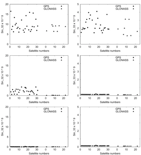
Sensitivity of GPS and GLONASS orbits with respect to resonant geopotential parameters
Texte intégral
Figure


Documents relatifs
In this section we test a second order algorithm for the 2-Wasserstein dis- tance, when c is the Euclidean cost. Two problems will be solved: Blue Noise and Stippling. We denote by
L’archive ouverte pluridisciplinaire HAL, est destinée au dépôt et à la diffusion de documents scientifiques de niveau recherche, publiés ou non, émanant des
From the previous representations of the solutions to the KPI equation given by the author, we succeed to give solutions to the CKP equation in terms of Fredholm determinants of
A comparative analysis of the spin parameters, as well as the spin entry/recovery behavior for the nominal and perturbed aerodynamic models, revealed the high sensitivity of
L’archive ouverte pluridisciplinaire HAL, est destinée au dépôt et à la diffusion de documents scientifiques de niveau recherche, publiés ou non, émanant des
There was a breakthrough two years ago, when Baladi and Vall´ee [2] extended the previous method for obtaining limit distributions, for a large class of costs, the so-called
AIUB tested the sensitivity of GOCE to temporal gravity field variations by (1) derivation of monthly solutions and (2) by estimation of mean annual amplitudes from
The contribution of these five attributes was examined by creating 6 models and comparing the results of each model with the results of the same model when the entire attribute
