HAL Id: inria-00170414
https://hal.inria.fr/inria-00170414
Submitted on 7 Sep 2007
HAL is a multi-disciplinary open access
archive for the deposit and dissemination of
sci-entific research documents, whether they are
pub-lished or not. The documents may come from
teaching and research institutions in France or
abroad, or from public or private research centers.
L’archive ouverte pluridisciplinaire HAL, est
destinée au dépôt et à la diffusion de documents
scientifiques de niveau recherche, publiés ou non,
émanant des établissements d’enseignement et de
recherche français ou étrangers, des laboratoires
publics ou privés.
Gregory Kucherov, Laurent Noé, Mihkail Roytberg
To cite this version:
Gregory Kucherov, Laurent Noé, Mihkail Roytberg. Subset seed automaton. CIAA 2007, Jul 2007,
Prague, Czech Republic. pp.180-191, �10.1007/978-3-540-76336-9_18�. �inria-00170414�
inria-00170414, version 1 - 7 Sep 2007
Gregory Kucherov1, Laurent No´e1, and Mikhail Roytberg2
1 LIFL/CNRS/INRIA, Bˆat. M3 Cit´e Scientifique, 59655, Villeneuve d’Ascq cedex,
France, {Gregory.Kucherov,Laurent.Noe}@lifl.fr
2 Institute of Mathematical Problems in Biology, Pushchino, Moscow Region,
142290, Russia, [email protected]
Abstract. We study the pattern matching automaton introduced in [1] for the purpose of seed-based similarity search. We show that our defini-tion provides a compact automaton, much smaller than the one obtained by applying the Aho-Corasick construction. We study properties of this automaton and present an efficient implementation of the automaton construction. We also present some experimental results and show that this automaton can be successfully applied to more general situations.
1
Introduction
The technique of spaced seeds for similarity search in strings (sequences) was introduced about five years ago [2,3] and constituted an important algorithmic development [4,5]. Its main applications have been approximate string matching [2] and local alignment of DNA sequences [3,6,7] but the underlying idea applies also to other algorithmic problems on strings [8,9].
Since the invention of spaced seeds, different generalizations have been pro-posed, such as seeds with match errors [10,11], daughter seeds [12], indel seeds [13], or vector seeds [14]. In [1], we proposed the notion of subset seeds and demonstrated its advantages and its usefulness for DNA sequence alignment. In the formalism of subset seeds, an alignment is viewed as a text over some alphabet A, and a seed as a pattern over a subset alphabet B ⊆ 2A. The only
requirements made is that A contains a special letter 1, B contains a letter # = {1}, and every letter of B contains 1 in its set. The matching relation is naturally defined: a seed letter b ∈ B matches a letter a ∈ A iff a belongs to the set b.
For any seed-based similarity search method, including all above-mentioned types of seeds, an important issue is an accurate estimation of the sensitivity of a seed with respect to a given probabilistic model of alignments. For different probabilistic models, this problem has been studied in [15,16,17]. In [1] we pro-posed a general framework for this problem that allows one to compute the seed sensitivity for different definitions of seed and different alignment models. This approach is based on a finite automata representation of the set of target align-ments and the set of alignalign-ments matched by a seed, as well as on a representation of the probabilistic model of alignments as a finite-state transducer.
A key ingredient of the approach of [1] is a finite automaton that recognizes the set of alignments matched (or hit) by a given subset seed. We call this au-tomaton a subset seed auau-tomaton. The size (number of states) of the subset seed automaton is crucial for the efficiency of the whole algorithm of [1]. Note that the algorithm of [16] is also based on an automaton construction, namely on the Aho-Corasick automaton implied by the well-known string matching algorithm. Besides its application to the seeding technique for similarity search and string matching, constructing an efficient subset seed automaton is an interesting problem in its own, as it provides a solution to a variant of the subset matching problem studied in literature [18,19,20].
In this paper, we study properties of the subset seed automaton and present an efficient implementation of its construction. More specifically, we obtain the following results:
– we present a construction of subset seed automaton that has O(w2s−w)
states, compared to O(w|A|s−w) implied by the Aho-Corasick construction,
where s and w are respectively the span and the weight of the seed defined in the next Section,
– we further motivate our construction by showing that for some seeds, our construction gives the minimal automaton,
– we prove that our automaton is always smaller than the one obtained by the Aho-Corasick construction; we provide experimental data that confirm that for |A| = 2, our automaton is on average about 1.3 times bigger than the minimal one, while the Aho-Corasick automaton is about 2.5 times bigger. For |A| = 3 the difference is much more substantial: while our automaton is still about 1.3 times bigger than the minimal one, the Aho-Corasick au-tomaton turns out to be about 17 times bigger,
– we provide an efficient algorithm that implements the construction of the automaton such that each transition is computed in constant time,
– we show that our construction can be applied to the case of multiple seeds and to the general subset matching problem.
The presented automaton construction is implemented in full generality in Hedera software package (http//bioinfo.lifl.fr/yass/hedera.php) and has been applied to the design of efficient seeds for the comparison of genomic sequences.
2
Subset seed matching
The goal of seeds is to specify short string patterns that, if shared by two strings, have best chances to belong to a larger similarity region common to the two strings. To formalize this, a similarity region is modeled by an alignment between two strings. Usually one considers gapless alignments that, in the simplest case, are viewed as sequences of matches and mismatches and are easily specified by binary strings {0, 1}∗, where 1 is interpreted as “match” and 0 as “mismatch”.
its span and the number of # is called its weight. A spaced seed π ∈ {#, }s
matches (or hits) an alignment A ∈ {0, 1}∗ at a position p if for all i ∈ [1..s],
π[i] = # implies A[p + i − 1] = 1.
In [1], we proposed a generalization of this basic framework, based on the idea to distinguish between different types of mismatches in the alignments. This leads to representing both alignments and seeds as words over larger alphabets. In the general case, consider an alignment alphabet A of arbitrary size. We always assume that A contains a symbol 1, interpreted as “match”. A subset seed is defined as a word over a seed alphabet B, such that
– each letter b ∈ B denotes a subset of A that contains 1 (b ∈ 2A\ 2A\{1}),
– B contains a letter # that denotes subset {1}.
As before, s is called the span of π, and the #-weight of π is the number of # in π. A subset seed π ∈ Bsmatches an alignment A ∈ A∗ at a position p iff for
all i ∈ [1..s], A[p + i − 1] ∈ π[i].
Example 1. For DNA sequences over the alphabet {A, C, G, T}, in [21] we consid-ered the alignment alphabet A = {1, h, 0} representing respectively a match, a transition mismatch (A ↔ G, C ↔ T), or a transversion mismatch (other mis-match). In this case, the appropriate seed alphabet is B = {#, @, } correspond-ing respectively to subsets {1}, {1, h}, and {1, h, 0}. Thus, seed π = #@ # matches alignment A = 10h1h1101 at positions 4 and 6. The span of π is 4, and the #-weight of π is 2.
One can view the problem of finding seed occurrences in an alignment as a special string matching problem. In particular, it can be considered as a special case of subset matching [18] where the text is composed of individual characters. It is also an instance of the problem of matching in indeterminate (degenerate) strings [19,20]. Therefore, an efficient automaton construction that we present in the following sections applies directly to these instances of string matching. One can also freely use the string matching terminology by replacing words “seed” and “alignment” by “pattern” and “text” respectively.
3
Subset Seed Automaton
Let us fix an alignment alphabet A, a seed alphabet B, and a seed π = π1. . . πs∈
B∗ of span s and #-weight w. Denote r = s − w and let R
π, |Rπ| = r, be
the set of all non-# positions in π. Throughout the paper, we identify each position z ∈ Rπ with the corresponding prefix π1..z = π1. . . πz of π, and we
interchangeably regard elements of Rπ as positions or as prefixes of π.
We now define an automaton Sπ=< Q, q0, QF, A, ψ : Q × A → Q >, q0∈ Q,
QF ⊆ Q, that recognizes the set of all alignments matched by π. The states
Q are defined as pairs hX, ti such that X = {x1, . . . , xk} ⊆ Rπ, t ∈ [0 . . . s],
max{X} + t ≤ s. The automaton maintains the following invariant condition. Suppose that Sπ has read a prefix a1. . . ap of an alignment A and has come to
1i, i ≤ s, and X contains all positions x
i∈ Rπ such that prefix π1..xi matches a
suffix of a1· · · ap−t. (a) π = #@# ## ### (b) A =111h1011h11 (c) a9t 111h1011h11 π1..7= #@# ## π1..4= #@# π1..2= #@ Fig. 1. Illustration to Example 2
Example 2. In the framework of Example 1, consider a seed π and an alignment prefix A = a1. . . ap of length p = 11 given in Figure 1(a) and (b) respectively.
The length t of the last run of 1’s of A is 2. The last non-1 letter of A is a9= h.
The set Rπ of non-# positions of π is {2, 4, 7} and π has 3 prefixes belonging
to Rπ (Figure 1(c)). Prefixes π1..2 and π1..7 do match suffixes of a1a2. . . a9, but
prefix π1..4 does not. Thus, the state of the automaton after reading a1a2. . . a11
is h{2, 7}, 2i.
The initial state q0 of Sπ is the state h∅, 0i. Final states QF of Sπ are all
states q = hX, ti, where max{X} + t = s. All final states are merged into one state hi.
The transition function ψ(q, a) is defined as follows. If q is a final state, then ∀a ∈ A, ψ(q, a) = q. If q = hX, ti is a non-final state, then
– if a = 1 then ψ(q, a) = hX, t + 1i, – otherwise ψ(q, a) = hXU∪ XV, 0i with
• XU = {x | x ≤ t + 1 and a ∈ πx}
• XV = {x + t + 1 | x ∈ X and a ∈ πx+t+1}
Example 3. Still in the framework of Example 1, consider seed π = # @#. Then the set Rπ is {2, 3}. Possible non-final states hX, ti of Sπ are states h∅, 0i, h∅, 1i,
h∅, 2i, h∅, 3i, h{2}, 0i, h{2}, 1i, h{3}, 0i, h{2, 3}, 0i. All these states are reachable in Sπ. Figure 2 shows the resulting automaton.
We now study main properties of automaton Sπ.
Lemma 1. The automaton Sπ accepts all alignments A ∈ A∗ matched by π.
Proof. It can be verified by induction that the invariant condition on the states hX, ti ∈ Q is preserved by the transition function ψ. The final state verifies max{X} + t = s which implies that at the first time Sπ gets into the final state,
π matches a suffix of a1. . . ap. ⊓⊔
Lemma 2. The number of states of the automaton Sπis no more than (w+1)2r,
where w is the #-weight of π.
Proof. Assume that Rπ = {z1, z2, . . . , zr} and z1< z2· · · < zr. Let Qibe the set
of non-final states hX, ti with max{X} = zi. For states q = hX, ti ∈ Qithere are
2i−1possible values of X and s − z
ipossible values of t between 0 and s − zi− 1,
as max{X} + t ≤ s − 1.
Thus, |Qi| ≤ 2i−1(s − zi) ≤ 2i−1(s − i), and (1) r X i=1 |Qi| ≤ r X i=1 2i−1(s − i) = (s − r + 1)2r− s − 1. (2)
Besides states Qi, Q contains s states h∅, ti (t ∈ [0..s − 1]) and one final state.
q0 q1 q2 q3 q4 q5 q6 q7 qf X= ∅ t= 0 X= ∅ t= 1 X= {2} t= 0 X= ∅ t= 2 X= {3} t= 0 X= {2} t= 1 X= {2, 3} t= 0 X= ∅ t= 3 1 0 h 1 1 0 h 1 0,h 1 0 h 1 0,h 1 0,h 0 h 1 0,h 0,h,1
Fig. 2. Illustration to Example 3
Note that if π starts with #, which is always the case for spaced seeds, then Xi ≥ i + 1, i ∈ [1..r], and the bound of (1) rewrites to 2i−1(s − i − 1). This
results in the same w2r bound on number of states as the one for the
Aho-Corasick automaton proposed in [16] for spaced seeds (see also Lemma 4 below). The next Lemma shows that the construction of automaton Sπ is optimal in
the sense that no two states can be merged in general.
Lemma 3. Let A = {0, 1} and B = {#, }, where # = {1} and = {0, 1}. Consider a seed π = # · · · # with r letters ’ ’ between two #’s. Then the automaton Sπ is reduced, that is
(i) each of its states q is reachable, and
(ii) any two non-final states q′, q′′ are not equivalent.
Proof. (i) Let q = hX, ti be a non-final state of the automaton Sπ, and let X =
{x1, . . . , xk} with x1< · · · < xk. Let A = a1. . . axk∈ {0, 1}∗be an alignment of
length xk defined as follows: ap= 1 if, for some i ∈ [1..k], p = xk− xi+ 1, and
ap= 0 otherwise. Note that 1 /∈ X and thus axk = 0. Thus ψ(h∅, 0i, A) = hX, 0i
and finally ψ(h∅, 0i, A · 1t) = q.
(ii) For a set X = {x1, . . . , xk} and an integer t, denote X ⊕ t = {x1+
t, . . . , xk+ t}. Let q′ = hX′, t′i and q′′ = hX′′, t′′i be non-final states of Sπ. If
max{X′} +t′ > max{X′′} +t′′, then let d = (r + 2)− (max{X′} +t′). Obviously,
ψ(q′, 1d) is a final state, and ψ(q′′, 1d) is not.
Now assume that max{X′} + t′ = max{X′′} + t′′. Let g = max{v|(v ∈
X′⊕ t′ and v /∈ X′′⊕ t′′) or (v ∈ X′′⊕ t′′ and v /∈ X′⊕ t′)}. By symmetry,
assume that the maximum is reached on the first condition, i.e. g = x′
some x′
i ∈ X′. Let d = (r + 1) − g and consider word 0d1. It is easy to see that
ψ(q′, 0d1) is a final state. We claim that ψ(q′′, 0d1) is not. To see this, observe
that none of the seed prefixes corresponding to x ∈ X′′with x + t′′> x′i+ t′can
lead to the final state on 0d1, due to the last # symbol of π. The details are left
to the reader. ⊓⊔
Another interesting property of Sπ is the existence of a surjective mapping
from the states of the Aho-Corasick automaton onto reachable states of Sπ.
This mapping proves that even if Sπ is not always minimized, it has always a
smaller number of states than the Corasick automaton. Here, by the Aho-Corasick (AC) automaton, we mean the automaton with the states corresponding to nodes of the trie built according to the classical Aho-Corasick construction [22] from the set of all instances of the seed π. More precisely, given a seed π of span s, the set of states of the AC-automaton is QAC = {A ∈ A∗| |A| ≤
s and A is matched by prefix π1..|A|}. The transition ψ(A, a) for A ∈ QAC, a ∈
A yields the longest A′∈ Q
AC which is a suffix of Aa. We assume that all final
states are merged into a single sink state.
Lemma 4. Consider an alignment alphabet A, a seed alphabet B and a seed π ∈ Bs of span s. There exists a surjective mapping f : Q
AC → Q from the
set of states of the Aho-Corasick automaton to the set of reachable states of the subset seed automaton Sπ.
Proof. We first define the mapping f . Consider a state A ∈ QAC, |A| = p < s,
where A is matched by π1..p. Decompose A = A′1t, where the last letter of A′
is not 1. If A′ is empty, define f (A) = h∅, ti. Otherwise, π
1..p−t matches A′ and
π[p − t] 6= #. Let X be a set of positions that contains p − t together with all positions i < p − t such that π1..i matches a suffix of A′. Define f (A) = hX, ti. It
is easy to see that hX, ti ∈ Q, that hX, ti exists in Sπ and is reachable by string
A.
Now show that for every reachable state hX, ti ∈ Q of Sπ there exists A ∈
QAC such that f (A) = hX, ti. Consider a string C ∈ A∗ that gets Sπ to the
state hX, ti. Then C = C′1t and the last letter of C′ is not 1. If X is empty
then define A = 1t. If X is not empty, then consider the suffix A′ of C′ of length
x = max{X} and define A = A′1t. Since π
1..x matches A′, and x + t ≤ s, then
π1..x+tmatches A and therefore A ∈ QAC. It is easy to see that f (A) = hX, ti.
⊓ ⊔ Observe that the mapping of Lemma 4 is actually a morphism from the Aho-Corasick automaton to Sπ.
Table 1 shows experimentally estimated average sizes of the Aho-Corasick automaton, subset seed automaton, and minimal automaton. The two tables correspond respectively to the binary alphabet (spaced seeds) and ternary al-phabet (see Example 1). For Aho-Corasick and subset seed automata, the ratio to the average size of the minimal automaton is shown. Each line corresponds to a seed weight (#-weight for |A| = 3). In each case, 10000 random seeds of different span have been generated to estimate the average.
|A| = 2 Aho-Corasick Sπ Minimized w avg. ratio avg. ratio avg. 9 130.98 2.46 67.03 1.260 53.18 10 140.28 2.51 70.27 1.255 55.98 11 150.16 2.55 73.99 1.254 58.99 12 159.26 2.57 77.39 1.248 62.00 13 168.19 2.59 80.92 1.246 64.92
|A| = 3 Aho-Corasick Sπ Minimized w avg. ratio avg. ratio avg. 9 1103.5 16.46 86.71 1.293 67.05 10 1187.7 16.91 90.67 1.291 70.25 11 1265.3 17.18 95.05 1.291 73.65 12 1346.1 17.50 98.99 1.287 76.90 13 1419.3 17.67 103.10 1.284 80.31
Table 1. Average number of states of Aho-Corasick, Sπand minimal automaton
4
Subset seed automaton implementation
As in section 3, consider a subset seed π of #-weight w and span s, and let r = s − w be the number of non-# positions. A straightforward generation of the transition table of the automaton Sπcan be performed in time O(r·w·2r·|A|).
In this section, we show that Sπ can be constructed in time proportional to its
size, which is bounded by (w +1)2r, according to Lemma 2. In practice, however,
the number of states is usually much smaller.
The algorithm generates the states of the automaton incrementally by travers-ing them in the breadth-first manner. Transitions ψ(hX, ti, a) are computed us-ing previously computed transitions ψ(hX′, ti, a). A tricky part of the algorithm
corresponds to the case where state ψ(hX, ti, a) has already been created before and should be retrieved.
The whole construction of the automaton is given in Algorithm 1. We now describe it in more details.
Let Rπ = {z1, . . . , zr} and z1 < z2· · · < zr. Consider X ⊆ Rπ. To retrieve
the maximal element of X, the algorithm maintains a function k(X) defined by k(X) = max{i|zi∈ X}, k(∅) = 0.
Let q = hX, ti be a non-final and reachable state of Sπ, X = {x1, . . . , xi} ⊆
Rπ and x1 < x2· · · < xi. We define X′ = X \ {zk(X)} = {x1, . . . , xi−1} and
q′ = hX′, ti. The following lemma holds.
Lemma 5. If q = hX, ti is reachable, then q′= hX′, ti is reachable and has been
processed before in a breadth-first computation of Sπ.
Proof. First prove that hX′, ti is reachable. If hX, ti is reachable, then hX, 0i
is reachable due to the definition of transition function for t > 0. Thus, there is a word A of length xi = zk(X) such that ∀j ∈ [1..r], zj ∈ X iff the seed
suffix π1..zj matches the word suffix Axi−zj+1· · · Axi. Define A′ to be the suffix
of A of length xi−1= zk(X′)and observe that reading A′ gets the automaton to
the state hX′, 0i, and then reading A′· 1t leads to the state hX′, ti. Finally, as
|A′·1t| < |A·1t|, then the breadth-first traversal of states of A
πalways processes
state hX′, ti before hX, ti. ⊓⊔
To retrieve X′ from X, the algorithm maintains a function Fail(q), similar
to the failure function of the Aho-Corasick automaton, such that Fail(hX, ti) = hX′, ti for X 6= ∅, and Fail(h∅, ti) = h∅, max{t − 1, 0}i.
We now explain how values ψ(q, a) are computed by Algorithm 1. Note first that if a = 1, state ψ(q, a) = hX, t + 1i can be computed in constant time (part a. of Algorithm 1). Moreover, since this is the only way to reach state hX, t + 1i, it is created and added once to the set of states.
Assume now that a 6= 1. To compute ψ(q, a) = hY, 0i, we retrieve state q′ = Fail(q) = hX′, ti and then retrieve ψ(q′, a) = hY′, 0i. Note that this is
well-defined as by Lemma 5, q′ has been processed before q.
Observe now that since X′ and X differ by only one seed prefix π 1..zk(X)
the only possible difference between Y and Y′ can be the prefix π
1..zk(X)+t+1
depending on whether πzk(X)+t+1matches a or not. As a 6= 1, this is equivalent to
testing whether (zk(X)+ t + 1) ∈ Rπand πzk(X)+t+1matches a. This information
can be precomputed for different values k(X) and t. For every a 6= 1, we define
V (k, t, a) = (
{zk+ t + 1} if zk+ t + 1 ∈ Rπ and πzk+t+1matches a,
∅ otherwise.
Thus, Y = Y′∪ V (k(X), t, a) (part c. of Algorithm 1). Function V (k, t, a) can
be precomputed in time and space O(|A| · r · s).
Note that if V (k, t, a) is empty, then hY, 0i is equal to an already created state hY′, 0i and no new state needs to be created in this case (part e. of Algorithm 1).
If V (k, t, a) is not empty, we need to find out if hY, 0i has already been created or not and if it has, we need to retrieve it. To do that, we need an additional construction. For each state q′ = hX′, ti, we maintain another
func-tion RevMaxFail(q′), that gives the last created state q = hX, ti such that
X\zk(X) = X′ (part d. of Algorithm 1). Since the state generation is
breadth-first, new states hX, ti are created in a non-decreasing order of the quantity (zk(X)+ t). Therefore, among all states hX, ti such that Fail(hX, ti) = hX′, ti,
RevMaxFail(hX′, ti) returns the one with the largest zk(X). Now, observe that if V (k, t, a) is not empty, i.e. Y = Y′∪ {z
k(X)+ t + 1},
then Fail(hY, 0i) = hY′, 0i. Since state hY, 0i has the maximal possible current
value zk(Y )+ 0 = zk(X)+ t + 1, by the above remark, we conclude that if hY, 0i
has already been created, then RevMaxFail(hY′, 0i) = hY, 0i. This allows us
to check if this is indeed the case and to retrieve the state hY, 0i if it exists (part d. of Algorithm 1).
The generation of states hX, ti with X = ∅ represents a special case (part b. of Algorithm 1). Here another precomputed function is used:
U (t, a) gives the set of seed prefixes that match the word 1t· a. In this case,
checking if resulting states have been already added is done in a similar way to V (k, t, a). Details are left out.
Algorithm 1: computation of Sπ
Data: a seed π = π1π2. . . πs
Result: an automaton Sπ= hQ, q0, qF,A, ψi
qF ← createstate(hi); q0← createstate(h∅, 0i);
/* process the first level of states to set Fail and RevMaxFail */ for a ∈ A do if a ∈ π1 then if a = 1 then hY, tyi ← h∅, 1i; else hY, tyi ← h{1}, 0i; if zk(Y )+ ty≥ s then qy← qF; else qy← createstate(hY, tyi); Fail(qy) ← q0; RevMaxFail(q0) ← qy; push(Queue, qy); else qy← q0; ψ(q0, a) ← qy; /* breadth-first processing */ while Queue 6= ∅ do q: hX, tXi ← pop(Queue); q′← Fail(q); for a ∈ A do /* compute ψ(hX, tXi, a) = hY, tyi */ q′ y: hY′, t′yi ← ψ(q′, a); if a = 1 then Y ← X; a ty← tX+ 1; else if X = ∅ then b Y ← U (tX, a); else c Y ← Y′∪ V (k(X), tX, a); ty← 0;
/* create a new state unless it already exists or it is final */ qrev: hYrev, trevi ← RevMaxFail(qy′);
if def ined(qrev) and ty= trev and Y = Yrev then
d qy← qrev;
else if ty= t′yand Y = Y′then
e qy← q′ y; else if zk(Y )+ ty≥ s then qy← qF; else qy← createstate(hY, tyi); Fail(qy) ← q′ y; RevMaxFail(qy′) ← qy; push(Queue, qy); ψ(q, a) ← qy;
We summarize the results of this section with the following Lemma.
Lemma 6. After a preprocessing of seed π within time O(|A|·s2), the automaton
Sπ can be constructed by incrementally generating all reachable states so that
every transition ψ(q, a) is computed in constant time.
5
Possible extensions
An important remark is that the automaton defined in this paper can be easily generalized to the case of multiple seeds. For seeds π1, . . . , πk, a state of the
automaton recognizing the alignments matched by one of the seeds would be a tuple < X1, . . . , Xk, t >, where X1, . . . , Xkcontain the set of respective prefixes,
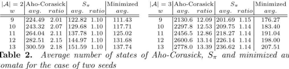
similarly to the construction of the paper. Interestingly, Lemma 4 still holds for the case of multiple seeds. This means that although the size of the union of individual seed automata could potentially grow as the product of sizes, it actually does not, as it is bounded by the size of the Aho-Corasick automaton which grows additively with respect to subsets of underlying words. In practice, our automaton is still substantially smaller than the Aho-Corasick automaton, as illustrated by Table 2. Similar to Table 1, 10000 random seed pairs have been generated here in each case to estimate the average size.
|A| = 2 Aho-Corasick Sπ Minimized w avg. ratio avg. ratio avg.
9 224.49 2.01 122.82 1.10 111.43 10 243.32 2.07 129.68 1.10 117.71 11 264.04 2.11 137.78 1.10 125.02 12 282.51 2.15 144.97 1.10 131.68 13 300.59 2.18 151.59 1.10 137.74
|A| = 3 Aho-Corasick Sπ Minimized w avg. ratio avg. ratio avg. 9 2130.6 12.09 201.69 1.15 176.27 10 2297.8 12.53 209.75 1.14 183.40 11 2456.5 12.86 218.27 1.14 191.04 12 2600.6 13.14 226.14 1.14 198.00 13 2778.0 13.39 236.62 1.14 207.51
Table 2. Average number of states of Aho-Corasick, Sπ and minimized
au-tomata for the case of two seeds
Another interesting observation is that the construction of a matching au-tomaton where each state is associated with a set of “compatible” prefixes of the pattern is a general one and can be applied to the general problem of subset matching [18,23,19,20]. Recall that in subset matching, a pattern is composed of subsets of alphabet letters. This is the case, for example, with IUPAC genomic motifs, such as motif ANDGR representing the subset motif A[ACGT ][AGT ]G[AG].
Note that the text can also be composed of subset letters, with two possible matching interpretations [20]: a seed letter b matches a text letter a either if a ⊆ b or if a ∩ b 6= ∅.
Interestingly, the automaton construction of this paper still applies to these cases with minor modifications due to the absence of text letter 1 matched by any seed letter. With this modification, the automaton construction algo-rithm of Section 4 still applies. As a test case, we applied it to subset motif
[GA][GA]GGGN N N N AN [CT ]AT GN N [AT ]N N N N N [CT G]mentioned in [20] as a motif
describing the translation initiation site in the E.coli genome. For a regular 4-letters genomic text, the automaton obtained with our approach has only 138 states, while the minimal automaton has 126 states. For a text composed of 15
subsets of 4 letters and the inclusion matching relation, our automaton contains 139 states, compared to 127 states of the minimal automaton. However, in the case of intersection matching relation, the automaton size increases drastically: it contains 87617 states compared to the 10482 states of the minimal automaton.
References
1. Kucherov, G., No´e, L., Roytberg, M.: A unifying framework for seed sensitivity and its application to subset seeds. JBCB 4(2) (2006) 553–569
2. Burkhardt, S., K¨arkk¨ainen, J.: Better filtering with gapped q-grams. Fundamenta Informaticae 56(1-2) (2003) 51–70
3. Ma, B., Tromp, J., Li, M.: PatternHunter: Faster and more sensitive homology search. Bioinformatics 18(3) (2002) 440–445
4. Brown, D., Li, M., Ma, B.: A tutorial of recent developments in the seeding of local alignment. JBCB 2(4) (2004) 819–842
5. Brown, D.: A survey of seeding for sequence alignments. In: Bioinformatics Algo-rithms: Techniques and Applications. (2007) to appear.
6. Li, M., Ma, B., Kisman, D., Tromp, J.: PatternHunter II: Highly sensitive and fast homology search. Journal of Bioinformatics and Computational Biology 2(3) (2004) 417–439
7. No´e, L., Kucherov, G.: YASS: enhancing the sensitivity of DNA similarity search. Nucleic Acids Research 33 (web-server issue) (2005) W540–W543
8. Califano, A., Rigoutsos, I.: Flash: A fast look-up algorithm for string homology. In: Proceedings of the 1st International Conference on Intelligent Systems for Molec-ular Biology (ISMB). (1993) 56–64
9. Tsur, D.: Optimal probing patterns for sequencing by hybridization. In: Proc. 6th Workshop on Algorithms in Bioinformatics (WABI). Volume 4175 of LNCS. (2006) 366–375
10. Schwartz, S., Kent, J., Smit, A., Zhang, Z., Baertsch, R., Hardison, R., Haussler, D., Miller, W.: Human–mouse alignments with BLASTZ. Genome Research 13 (2003) 103–107
11. Sun, Y., Buhler, J.: Choosing the best heuristic for seeded alignment of DNA sequences. BMC Bioinformatics 7(133) (2006)
12. Cs¨ur¨os, M., Ma, B.: Rapid homology search with two-stage extension and daughter seeds. In: Proceedings of the 11th International Computing and Combinatorics Conference (COCOON). Volume 3595 of LNCS. (2005) 104–114
13. Mak, D., Gelfand, Y., Benson, G.: Indel seeds for homology search. Bioinformatics 22(14) (2006) e341–e349
14. Brejov´a, B., Brown, D., Vinar, T.: Vector seeds: An extension to spaced seeds. Journal of Computer and System Sciences 70(3) (2005) 364–380
15. Keich, U., Li, M., Ma, B., Tromp, J.: On spaced seeds for similarity search. Discrete Applied Mathematics 138(3) (2004) 253–263 preliminary version in 2002. 16. Buhler, J., Keich, U., Sun, Y.: Designing seeds for similarity search in genomic
DNA. In: Proceedings of the 7th Annual International Conference on Computa-tional Molecular Biology (RECOMB). (2003) 67–75
17. Brejov´a, B., Brown, D., Vinar, T.: Optimal spaced seeds for homologous coding regions. Journal of Bioinformatics and Computational Biology 1(4) (2004) 595–610 18. Cole, R., Hariharan, R., Indyk, P.: Tree pattern matching and subset matching in deterministic O(n log3n)-time. In: Proceedings of 10th Symposium on Discrete
19. Holub, J., Smyth, W.F., Wang, S.: Fast pattern-matching on indeterminate strings. Journal of Discrete Algorithms (2006)
20. Rahman, S., Iliopoulos, C., Mouchard, L.: Pattern matching in degenerate DNA/RNA sequences. In: Proceedings of the Workshop on Algorithms and Com-putation (WALCOM). (2007) 109–120
21. No´e, L., Kucherov, G.: Improved hit criteria for DNA local alignment. BMC Bioinformatics 5(149) (2004)
22. Aho, A.V., Corasick, M.J.: Efficient string matching: An aid to bibliographic search. Communications of the ACM 18(6) (1975) 333–340
23. Amir, A., Porat, E., Lewenstein, M.: Approximate subset matching with don’t cares. In: Proceedings of 12th Symposium on Discrete Algorithms (SODA). (2001) 305–306