HAL Id: inserm-00405223
https://www.hal.inserm.fr/inserm-00405223
Submitted on 17 May 2010
HAL is a multi-disciplinary open access
archive for the deposit and dissemination of sci-entific research documents, whether they are pub-lished or not. The documents may come from teaching and research institutions in France or abroad, or from public or private research centers.
L’archive ouverte pluridisciplinaire HAL, est destinée au dépôt et à la diffusion de documents scientifiques de niveau recherche, publiés ou non, émanant des établissements d’enseignement et de recherche français ou étrangers, des laboratoires publics ou privés.
A Novel Split-Radix Fast Algorithm for 2-D Discrete
Hartley Transform
Longyu Jiang, Huazhong Shu, Jiasong Wu, Lu Wang, Lotfi Senhadji
To cite this version:
Longyu Jiang, Huazhong Shu, Jiasong Wu, Lu Wang, Lotfi Senhadji. A Novel Split-Radix Fast Algorithm for 2-D Discrete Hartley Transform. IEEE Transactions on Circuits and Systems Part 1 Fundamental Theory and Applications, Institute of Electrical and Electronics Engineers (IEEE), 2010, 57 (4), pp.911-924. �10.1109/TCSI.2009.2028639�. �inserm-00405223�
Abstract—This paper presents a fast split-radix-(2×2)/(8×8)
algorithm for computing the two-dimensional (2-D) discrete Hartley transform (DHT) of length N×N with N = q*2m, where q is an odd integer. The proposed algorithm decomposes an N×N DHT into one N/2×N/2 DHT and forty-eight N/8×N/8 DHTs. It achieves an efficient reduction on the number of arithmetic operations, data transfers and twiddle factors compared to the split-radix-(2×2)/(4×4) algorithm. Moreover, the characteristic of expression in simple matrices leads to an easy implementation of the algorithm. If implementing the above two algorithms with fully parallel structure in hardware, it seems that the proposed algorithm can decrease the area complexity compared to the split-radix-(2×2)/(4×4) algorithm, but requires a little more time complexity. An application of the proposed algorithm to 2-D medical image compression is also provided.
Index Terms—Two-dimensional (2-D) discrete Hartley transform (DHT), split-radix, fast algorithm
I. INTRODUCTION
he discrete Hartley transform (DHT) is widely used in signal and image processing applications. The advantage of the DHT over the discrete Fourier transform (DFT) is that it can be used to avoid complex operations when the input sequence is real. Moreover, the forward and inverse DHTs differ from each other in their form only in the scaling factor. Owing to these properties, the DHT is now finding an increasing interest in the signal processing community. In the
Manuscript received November 23, 2008. This work was supported by the National Natural Science Foundation of China under Grant 60873048, the Program for Changjiang Scholars and Innovative Research Team in University and the Natural Science Foundation of Jiangsu Province of China under Grant BK2008279.
L. Jiang is with the Laboratory of Image Science and Technology, School of Computer Science and Engineering, Southeast University, Nanjing 210096, China (e-mail: [email protected]).
H. Shu and L. Wang are with the Laboratory of Image Science and Technology, School of Computer Science and Engineering, Southeast University, Nanjing 210096, China, and also with the Centre de Recherche en Information Biomédicale Sino-Français (CRIBs), Nanjing 210096, China (e-mail: [email protected]; [email protected]).
J. Wu is with the Laboratory of Image Science and Technology, School of Biological Science and Medical Engineering, Southeast University, Nanjing 210096, China, and with the Centre de Recherche en Information Biomédicale Sino-Français (CRIBs), Nanjing 210096, China, and with INSERM, U 642, 35000 Rennes, France, and with the Laboratoire Traitement du Signal et de l’Image (LTSI), Université de Rennes 1, 35000 Rennes, France, and also with the Centre de Recherche en Information Biomédicale Sino–Français (CRIBs), 35000 Rennes, France (e-mail: [email protected]).
L. Senhadji is with INSERM, U 642, 35000 Rennes, France, and with the Laboratoire Traitement du Signal et de l’Image (LTSI), Université de Rennes 1, 35000 Rennes, France, and also with the Centre de Recherche en Information Biomédicale Sino–Français (CRIBs), 35000 Rennes, France (e-mail:
past decades, fast algorithms and implementations of one-dimensional (1-D) DHT and DFT have been extensively investigated [1]-[21]. Meantime, special attention has also been paid on the two-dimensional (2-D) and three-dimensional (3-D) DHT [22]-[39], this is due to the growing interest in applications involving multi-dimensional (M-D) signals. In this paper, fast algorithm means lower computational complexity in terms of the number of arithmetic operations, data transfers and twiddle factors.
The algorithms proposed for fast computing the 2-D DHT can be classified into four categories: i) the row-column method; ii) the vector-radix fast Hartley transform (FHT) algorithms [22]-[24]; iii) the split-radix FHT algorithm [25]-[31]; and iv) the polynomial transform FHT algorithm [32]-[34]. The row-column method computes the 2-D DHT by taking the 1-D FHT sequentially along each dimension of the input data while in the vector-radix algorithm, the 2-D DHT is decomposed into many smaller ones until the trivial sequence length is reached. The vector-radix method reduces the number of arithmetic operations over the row-column algorithm and possesses the desirable properties such as regular structure and low implementation cost. This approach was then extended to 3-D DHT [35]-[37] and M-D DHT [23]. In [39], a vector-radix-3×3 algorithm was developed for computing the 2-D DHT of sequence whose length is 3m×3m. The polynomial
transform based FHT algorithms for M-D DHT have been reported in [32] and [34], which lead to a great reduction of the arithmetic operations at the expense of very complicated structure. The split-radix 2-D DHT algorithm is more efficient than the vector-radix algorithm in terms of arithmetic complexity and it is easy to implement. All the split-radix algorithms for 2-D DHT reported so far are based on a mixture of radix-2×2 and radix-4×4 index maps.
Huang et al. [25] applied a radix-2×2 decomposition to the even-even, even-odd, odd-even indexed samples and a radix-4×4 decomposition to the odd-odd indexed samples. Thus, an N×N DHT is decomposed into three N/2×N/2 DHTs and four N/4×N/4 DHTs. By using a radix-4×4 decomposition to even-odd, odd-even and odd-odd indexed terms, an improved split-radix algorithm for 2-D DHT was further derived [28], which decomposes an N×N 2-D DHT into one N/2×N/2 DHT and twelve N/4×N/4 DHTs. The split-radix algorithms for the 2-D DHT have been presented using decimation-in-frequency (DIF) [29] and decimation-in-time (DIT) [30]. It seems that the algorithms reported in [29] and [30] are the most efficient ones among all the existing split-radix algorithms in terms of the arithmetic complexity.
A Novel Split-Radix Fast Algorithm for 2-D
Discrete Hartley Transform
Longyu Jiang, Huazhong Shu, Senior Member, IEEE, Jiasong Wu, Lu Wang and Lotfi Senhadji,
Senior Member, IEEE
Moreover, these two algorithms support various sequence lengths. Specifically, the block size can be chosen as q*2m×q*2m, where q is an odd integer. In [31], the radix-2/4
approach has been generalized to the M-D DHT. In particular, for the case of 2-D DHT, it has the same arithmetic complexity as that of the algorithms presented in [29] and [30].
Among all the algorithms mentioned above, the split-radix algorithms based on radix-2/4 are the most attractive ones because they provide a good comprise between the arithmetic and structural complexities. Recently, Bouguezel et al. [3] proposed a new split-radix fast algorithm based on a mixture of radix-2 and radix-8 index maps for 1-D DHT of sequences whose length is q×2m, where q is an odd integer. This algorithm
is more efficient than the conventional split radix-2/4 FHT algorithm in terms of the number of data transfers and twiddle factor evaluations, which also contribute significantly to the execution time of FHT algorithms. Inspired by the algorithm presented in [3], we propose a split-radix-(2×2)/(8×8) algorithm for computing the 2-D DHT of sequences with length-q*2m×q*2m, which consists of decomposing an N×N
DHT into one N/2×N/2 DHT and forty-eight N/8×N/8 DHTs. Besides, the split radix-2/8 algorithm has been already used for computing the 2-D DFT [40], [41].
The rest of the paper is organized as follows. Section II presents the derivation of the algorithm. In Section III, the computational complexity and the hardware area and time complexity of the proposed algorithm are analyzed, and the comparison with some existing algorithms is also provided. Section IV presents the result of software implementation of the proposed and some existing algorithms. Section V concludes the work.
II. PROPOSED RADIX-(2×2)/(8×8) ALGORITHM The 2-D DHT X(k1, k2) of real valued sequence, x(n1, n2), for 0 ≤ n1, n2 ≤ N – 1, is defined by 1 2 1 2 1 1 2 1 2 1 2 0 0 1 ( , ) 2 ( , )cas , 0 , 1, N N i i n n i X k k x n n n k k k N N π − − = = = ⎛ ⎞ = ⎜ ⎟ ≤ ≤ − ⎝ ⎠
∑ ∑
∑
(1)where cas( ) cos( ) sin( ).θ = θ + θ The sequence length N is assumed to be q×2m, where q is an odd integer and m > 0.
Let us first consider the case when m = 1, that is, N = 2q. A. The case m = 1, i.e., N = 2q
In this case, the radix-2×2 algorithm is used to decompose a length-2q×2q DHT. The even-even indexed outputs are obtained by 1 2 1 2 1 1 2 00 1 2 1 2 0 0 1 (2 , 2 ) 2 ( , )cas , 0 , 1. q q i i n n i X k k y n n n k k k q q π − − = = = ⎛ ⎞ = ⎜ ⎟ ≤ ≤ − ⎝ ⎠
∑ ∑
∑
(2)The even-odd, odd-even, and odd-odd indexed outputs can be computed by 1 1 2 2 1 2 1 2 1 1 2 2 1 1 2 ( ) 1 2 0 0 1 (2 , 2 ) 2 ( 1) ( , )cas , q q n p n p p p i i n n i X k p q k p q y n n n k q π − − + = = = + + ⎛ ⎞ = − ⎜ ⎟ ⎝ ⎠
∑ ∑
∑
(3) where p p1, 2 =0, 1, ( ,p p1 2) (0,0), 0≠ ≤k k1, 2≤ −q 1.The sequencesyp p1, 2( , )n n1 2 for p1, p2 = 0, 1, in (2) and (3) are obtained from the original input sequence as
(
)
(
)
00 1 2 01 1 2 10 1 2 11 1 2 2 2 1 2 1 2 1 2 1 2 ( , ), ( , ), ( , ), ( , ) ( ) ( , ), ( , ), ( , ), ( , ) T T y n n y n n y n n y n n H H x n n x n n q x n q n x n q n q = ⊗ + + + + (4) where T denotes the transpose, ⎥⎦ ⎤ ⎢ ⎣ ⎡ − = 1 1 1 1 2 H , and “⊗” is
the Kronecker product [42]. Fig. 1 shows the implementation of (4).
B. The case m = 2, i.e., N = 4q
When m = 2, the decomposition of (1) for the even-even indexed outputs is given by
1 2 1 2 2 1 2 1 2 2 / 4 00 1 2 1 2 0 0 1 (2 , 2 ) 2 ( , )cas , 0 , 2 1, 2 q q i i n n i X k k y n n n k k k q q π − − = = = ⎛ ⎞ = ⎜ ⎟ ≤ ≤ − ⎝ ⎠
∑ ∑
∑
(5) where 2 / 4 00 1 2 1 2 1 2 1 2 1 2 ( , ) [ ( , ) ( , 2 )] [ ( 2 , ) ( 2 , 2 )]. y n n x n n x n n q x n q n x n q n q = + + + + + + + (6)The even-odd, odd-even and odd-odd indexed outputs are obtained as follows 1 2 1 2 1 2 1 1 2 2 1 1 2 2 1 2 0 0 1 1 2 / 4 2 / 4 , 1 2 , 1 2 1 2 (4 , 4 ) 2 ( , )cas 2 ( , ) ( , ), 0 , 1, N N i i i i n n i i p p p p X k p q k p q x n n n k n p q F k k G k k k k q π π − − = = = = ± ± ⎛ ⎞ = ⎜ ± ⎟ ⎝ ⎠ = ± ≤ ≤ −
∑ ∑
∑
∑
(7) where 1 2 1 2 2 / 4 , 1 2 1 1 2 2 1 2 0 0 1 1 ( , ) 2 ( , ) cos cas , 2 p p N N i i i i n n i i F k k x n n n p n k q π π − − = = = = ⎛ ⎞ ⎛ ⎞ = ⎜ ⎟ ⎜ ⎟ ⎝ ⎠ ⎝ ⎠∑ ∑
∑
∑
(8) 1 2 1 2 2 / 4 , 1 2 1 1 2 2 1 2 0 0 1 1 ( , ) 2 ( , )sin cas . 2 p p N N i i i i n n i i G k k x n n n p n k q π π − − = = = = ⎛ ⎞ ⎛ ⎞ = ⎜ ⎟ ⎜− ⎟ ⎝ ⎠ ⎝ ⎠∑ ∑
∑
∑
(9)Using the matrix representation, (7) can be expressed as
1 2 1 2 1 1 2 2 1 1 2 2 2 / 4 , 1 2 2 2 / 4 , 1 2 ((4 ) mod 4 ,(4 ) mod 4 ) (( 4 ) mod 4 ,( 4 ) mod 4 ) ( , ) . ( , ) p p p p X k p q q k p q q X N k p q q N k p q q F k k H G k k + + ⎡ ⎤ ⎢ + − + − ⎥ ⎣ ⎦ ⎡ ⎤ = ⎢ ⎥ ⎢ ⎥ ⎣ ⎦ (10)
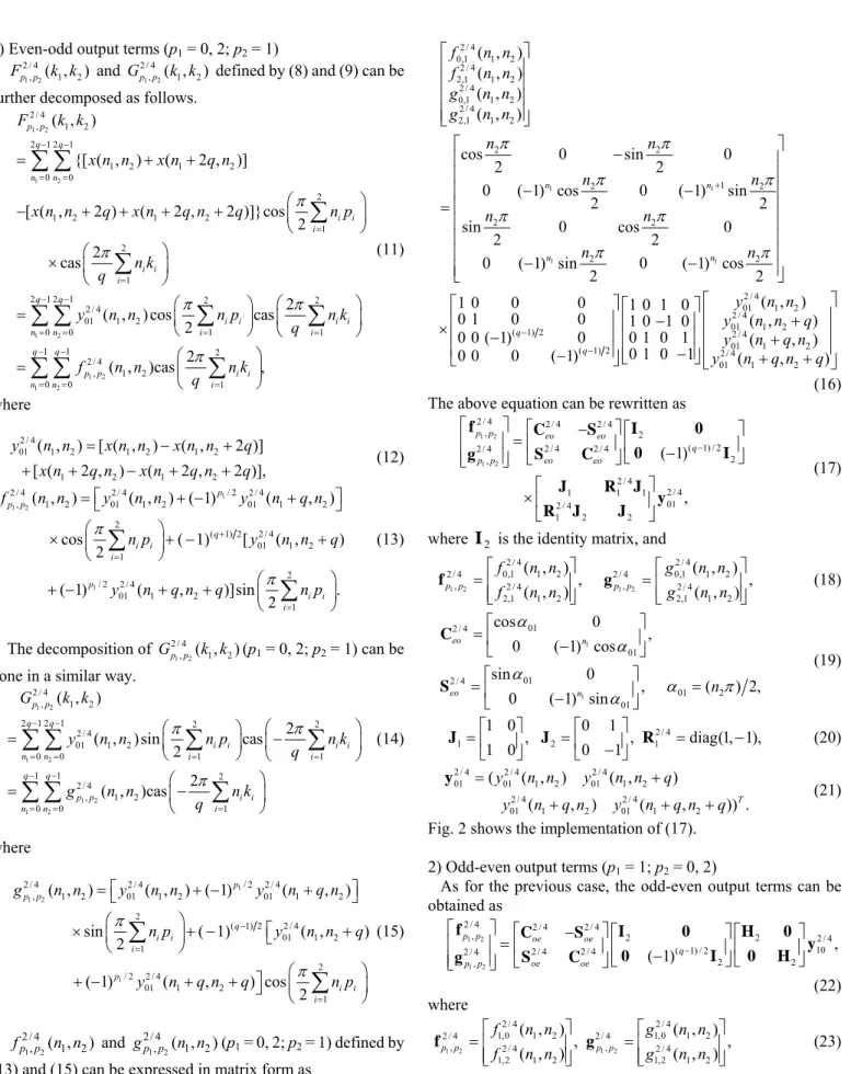
1) Even-odd output terms (p1 = 0, 2; p2 = 1) 1 2 2 / 4 , ( , )1 2 p p F k k and 2 / 41 2 , ( , )1 2 p p
G k k defined by (8) and (9) can be further decomposed as follows.
1 2 1 2 1 2 2 / 4 , 1 2 2 1 2 1 1 2 1 2 0 0 2 1 2 1 2 1 2 1 2 1 2 1 2 2 2 / 4 01 1 2 0 0 1 1 ( , ) {[ ( , ) ( 2 , )] [ ( , 2 ) ( 2 , 2 )]}cos 2 2 cas 2 ( , ) cos cas 2 p p q q n n i i i i i i q q i i i i n n i i F k k x n n x n q n x n n q x n q n q n p n k q y n n n p n k q π π π π − − = = = = − − = = = = = + + ⎛ ⎞ − + + + + ⎜ ⎟ ⎝ ⎠ ⎛ ⎞ × ⎜ ⎟ ⎝ ⎠ ⎛ ⎛ ⎞ = ⎜ ⎟ ⎜ ⎝ ⎠ ⎝
∑ ∑
∑
∑
∑ ∑
∑
∑
1 2 1 2 1 1 2 2 / 4 , 1 2 0 0 1 2 ( , )cas , q q p p i i n n i f n n n k q π − − = = = ⎞ ⎟ ⎠ ⎛ ⎞ = ⎜ ⎟ ⎝ ⎠∑ ∑
∑
(11) where 2 / 4 01 1 2 1 2 1 2 1 2 1 2 ( , ) [ ( , ) ( , 2 )] [ ( 2 , ) ( 2 , 2 )], y n n x n n x n n q x n q n x n q n q = − + + + − + + (12) 1 1 2 1 / 2 2 / 4 2 / 4 2 / 4 , 1 2 01 1 2 01 1 2 2 ( 1) 2 2 / 4 01 1 2 1 2 / 2 2 / 4 01 1 2 1 ( , ) ( , ) ( 1) ( , ) cos ( 1) [ ( , ) 2 ( 1) ( , )]sin . 2 p p p q i i i p i i i f n n y n n y n q n n p y n n q y n q n q n p π π + = = ⎡ ⎤ =⎣ + − + ⎦ ⎛ ⎞ × ⎜ ⎟+ − + ⎝ ⎠ ⎛ ⎞ + − + + ⎜ ⎟ ⎝ ⎠∑
∑
(13) The decomposition of 2 / 41 2 , ( , )1 2 p p G k k (p1 = 0, 2; p2 = 1) can be done in a similar way.1 2 1 2 1 2 1 2 2 / 4 , 1 2 2 1 2 1 2 2 2 / 4 01 1 2 0 0 1 1 1 1 2 2 / 4 , 1 2 0 0 1 ( , ) 2 ( , )sin cas 2 2 ( , )cas p p q q i i i i n n i i q q p p i i n n i G k k y n n n p n k q g n n n k q π π π − − = = = = − − = = = ⎛ ⎞ ⎛ ⎞ = ⎜ ⎟ ⎜− ⎟ ⎝ ⎠ ⎝ ⎠ ⎛ ⎞ = ⎜− ⎟ ⎝ ⎠
∑ ∑
∑
∑
∑ ∑
∑
(14) where 1 1 2 1 / 2 2 / 4 2 / 4 2 / 4 , 1 2 01 1 2 01 1 2 2 ( 1) 2 2 / 4 01 1 2 1 2 / 2 2 / 4 01 1 2 1 ( , ) ( , ) ( 1) ( , ) sin ( 1) ( , ) 2 ( 1) ( , ) cos 2 p p p q i i i p i i i g n n y n n y n q n n p y n n q y n q n q n p π π − = = ⎡ ⎤ =⎣ + − + ⎦ ⎛ ⎞ ⎡ × ⎜ ⎟+ − ⎣ + ⎝ ⎠ ⎛ ⎞ ⎤ + − + + ⎦ ⎜ ⎟ ⎝ ⎠∑
∑
(15) 1 2 2/ 4 , ( , )1 2 p p f n n and 1 2 2/ 4 , ( , )1 2 p p g n n (p1 = 0, 2; p2 = 1) defined by (13) and (15) can be expressed in matrix form as1 1 1 1 2 / 4 0,1 1 2 2 / 4 2,1 1 2 2 / 4 0,1 1 2 2 / 4 2,1 1 2 2 2 1 2 2 2 2 2 2 ( 1) ( , ) ( , ) ( , ) ( , ) cos 0 sin 0 2 2 0 ( 1) cos 0 ( 1) sin 2 2 sin 0 cos 0 2 2 0 ( 1) sin 0 ( 1) cos 2 2 1 0 0 0 0 1 0 0 0 0 ( 1) n n n n q f n n f n n g n n g n n n n n n n n n n π π π π π π π π + − ⎡ ⎤ ⎢ ⎥ ⎢ ⎥ ⎢ ⎥ ⎢ ⎥ ⎣ ⎦ ⎡ − ⎤ ⎢ ⎥ ⎢ ⎥ − − ⎢ ⎥ ⎢ ⎥ = ⎢ ⎥ ⎢ ⎥ ⎢ − − ⎥ ⎢ ⎥ ⎣ ⎦ × − 2 / 4 01 1 2 2 / 4 01 1 2 2 2 / 4 01 1 2 ( 1) 2 2 / 4 01 1 2 ( , ) 1 0 1 0 ( , ) 1 0 1 0 0 1 0 1 0 ( , ) 0 1 0 1 0 0 0 ( 1)q ( , ) y n n y n n q y n q n y n q n q − ⎡ ⎤ ⎡ ⎤ ⎡ ⎤ ⎢ ⎥ ⎢ ⎥⎢ − ⎥⎢ + ⎥ ⎢ ⎥ ⎢ ⎥⎢ + ⎥ ⎢ − ⎥ ⎢⎣ − ⎥⎦ + + ⎣ ⎦ ⎣ ⎦ (16) The above equation can be rewritten as
1 2 1 2 2 / 4 2 / 4 2 / 4 , 2 ( 1) / 2 2 / 4 2 / 4 2 / 4 2 , 2 / 4 2 / 4 1 1 1 01 2 / 4 1 2 2 ( 1) , p p eo eo q eo eo p p − ⎡ ⎤ ⎡ − ⎤⎡ ⎤ = ⎢ ⎥ ⎢ ⎥ ⎢ ⎥ − ⎢ ⎥ ⎣ ⎦⎣ ⎦ ⎣ ⎦ ⎡ ⎤ × ⎢ ⎥ ⎣ ⎦ f C S I 0 0 I S C g J R J y R J J (17)
where I2 is the identity matrix, and
1 2 1 2 2 / 4 2 / 4 0,1 1 2 0,1 1 2 2 / 4 2 / 4 , 2 / 4 , 2 / 4 2,1 1 2 2,1 1 2 ( , ) ( , ) , , ( , ) ( , ) p p p p f n n g n n f n n g n n ⎡ ⎤ ⎡ ⎤ =⎢ ⎥ =⎢ ⎥ ⎢ ⎥ ⎢ ⎥ ⎣ ⎦ ⎣ ⎦ f g (18) 1 1 01 2 / 4 01 01 2 / 4 01 2 01 cos 0 , 0 ( 1) cos sin 0 , ( ) 2, 0 ( 1) sin eo n eo n n α α α α π α ⎡ ⎤ = ⎢ − ⎥ ⎣ ⎦ ⎡ ⎤ =⎢ ⎥ = − ⎣ ⎦ C S (19) 2 / 4 1 2 1 1 0 0 1 , , diag(1, 1), 1 0 0 1 ⎡ ⎤ ⎡ ⎤ =⎢ ⎥ =⎢ ⎥ = − − ⎣ ⎦ ⎣ ⎦ J J R (20) 2 / 4 2 / 4 2 / 4 01 01 1 2 01 1 2 2 / 4 2 / 4 01 1 2 01 1 2 ( ( , ) ( , ) ( , ) ( , )) .T y n n y n n q y n q n y n q n q = + + + + y (21) Fig. 2 shows the implementation of (17).
2) Odd-even output terms (p1 = 1; p2 = 0, 2)
As for the previous case, the odd-even output terms can be obtained as 1 2 1 2 2 / 4 2 / 4 2 / 4 , 2 2 2 / 4 10 ( 1) / 2 2 / 4 2 / 4 2 / 4 2 2 , , ( 1) p p oe oe q oe oe p p − ⎡ ⎤ ⎡ − ⎤⎡ ⎤ ⎡ ⎤ = ⎢ ⎥ ⎢ ⎥ ⎢ ⎥ ⎢ ⎥ − ⎢ ⎥ ⎣ ⎦⎣ ⎦ ⎣ ⎦ ⎣ ⎦ f C S I 0 H 0 y 0 I 0 H S C g (22) where 1 2 1 2 2 / 4 2 / 4 1,0 1 2 1,0 1 2 2 / 4 2 / 4 , 2 / 4 , 2 / 4 1,2 1 2 1,2 1 2 ( , ) ( , ) , , ( , ) ( , ) p p p p f n n g n n f n n g n n ⎡ ⎤ ⎡ ⎤ =⎢ ⎥ =⎢ ⎥ ⎢ ⎥ ⎢ ⎥ ⎣ ⎦ ⎣ ⎦ f g (23)
2 2 10 2 / 4 10 10 2 / 4 10 1 10 cos 0 , 0 ( 1) cos sin 0 , ( ) 2, 0 ( 1) sin oe n oe n n α α α α π α ⎡ ⎤ = ⎢ − ⎥ ⎣ ⎦ ⎡ ⎤ =⎢ ⎥ = − ⎣ ⎦ C S (24) 2 / 4 2 / 4 2 / 4 10 10 1 2 10 1 2 2 / 4 2 / 4 10 1 2 10 1 2 ( ( , ) ( , ) ( , ) ( , )) ,T y n n y n n q y n q n y n q n q = + + + + y (25) 2 / 4 10 1 2 1 2 1 2 1 2 1 2 ( , ) [ ( , ) ( , 2 )] [ ( 2 , ) ( 2 , 2 )]. y n n x n n x n n q x n q n x n q n q = + + − + + + + (26)
3) Odd-odd output terms (p1 = 1, –1; p2 = 1)
We have the following decomposition for the odd-odd output terms 1 2 1 2 2 / 4 2 / 4 2 / 4 , 2 1 2 2 / 4 11 ( 1) / 2 2 / 4 2 / 4 2 / 4 2 / 4 2 / 4 2 1 2 2 1 , ( 1) p p oo oo q oo oo p p − ⎡ ⎤ ⎡ − ⎤⎡ ⎤ ⎡ ⎤ = ⎢ ⎥ ⎢ ⎥ ⎢ − ⎥ ⎢ ⎥ ⎢ ⎥ ⎣ ⎦⎣ ⎦ ⎣ ⎦ ⎣ ⎦ f C S I 0 J J y 0 I R J R J S C g (27) where 1 2 1 2 2 / 4 2 / 4 1,1 1 2 1,1 1 2 2 / 4 2 / 4 , 2 / 4 , 2 / 4 1,1 1 2 1,1 1 2 2 / 4 2 ( , ) ( , ) , , ( , ) ( , ) diag( 1,1), p p p p f n n g n n f n n g n n − − ⎡ ⎤ ⎡ ⎤ =⎢ ⎥ =⎢ ⎥ ⎢ ⎥ ⎢ ⎥ ⎣ ⎦ ⎣ ⎦ = − f g R (28) 11 11 2 / 4 2 / 4 11 11 11 2 1 11 1 2 cos 0 sin 0 , , 0 cos 0 sin [( ) ] 2, [( ) ] 2, oo oo n n n n α α α α α π α π ⎡ ⎤ ⎡ ⎤ =⎢ ⎥ =⎢ ⎥ ′ ′ ⎣ ⎦ ⎣ ⎦ ′ = − = + C S (29) 2 / 4 2 / 4 2 / 4 11 11 1 2 11 1 2 2 / 4 2 / 4 11 1 2 11 1 2 ( ( , ) ( , ) ( , ) ( , )) ,T y n n y n n q y n q n y n q n q = + + + + y (30) 2 / 4 11 1 2 1 2 1 2 1 2 1 2 ( , ) [ ( , ) ( , 2 )] [ ( 2 , ) ( 2 , 2 )]. y n n x n n x n n q x n q n x n q n q = − + − + − + + (31) C. The case m ≥ 3
By introducing a mixture of radix-2×2 and radix-8×8 index maps, we propose a novel decomposition of (1). The even-even output terms can be computed by
1 2 1 2 2 1 2 1 2 2 / 8 00 1 2 1 2 0 0 1 (2 , 2 ) 2 ( , )cas , 0 , 2 1, 2 N N i i n n i X k k y n n n k k k N N π − − = = = ⎛ ⎞ = ⎜ ⎟ ≤ ≤ − ⎝ ⎠
∑ ∑
∑
(32) where 2 / 8 00 1 2 1 2 1 2 1 2 1 2 ( , ) [ ( , ) ( , 2)] [ ( 2, ) ( 2, 2)]. y n n x n n x n n N x n N n x n N n N = + + + + + + + (33)The even-odd, odd-even, and odd-odd output terms can be derived as follows. 1 2 1 2 1 2 1 1 2 2 1 1 2 2 1 2 0 0 1 1 2 / 8 2 / 8 , 1 2 , 1 2 1 2 (8 ,8 ) 2 2 ( , )cas 8 ( , ) ( , ), 0 , 8 1, N N i i i i n n i i p p p p X k p q k p q x n n n k n p N N q F k k G k k k k N π π − − = = = = ± ± ⎛ ⎞ = ⎜ ± ⎟ ⎝ ⎠ = ± ≤ ≤ −
∑ ∑
∑
∑
(34) where 1 2 1 2 2 / 8 , 1 2 1 1 2 2 1 2 0 0 1 1 ( , ) 2 2 ( , ) cos cas , 8 p p N N i i i i n n i i F k k x n n n p n k N q N π π − − = = = = ⎛ ⎞ ⎛ ⎞ = ⎜ ⎟ ⎜ ⎟ ⎝ ⎠ ⎝ ⎠∑ ∑
∑
∑
(35) 1 2 1 2 2 / 8 , 1 2 1 1 2 2 1 2 0 0 1 1 ( , ) 2 2 ( , )sin cas . 8 p p N N i i i i n n i i G k k x n n n p n k N q N π π − − = = = = ⎛ ⎞ ⎛ ⎞ = ⎜ ⎟ ⎜− ⎟ ⎝ ⎠ ⎝ ⎠∑ ∑
∑
∑
(36)Equation (34) can be written in matrix form as
1 2 1 2 1 1 2 2 1 1 2 2 2 / 8 , 1 2 2 2 / 8 , 1 2 ((8 ) mod ,(8 ) mod ) (( 8 ) mod ,( 8 ) mod ) ( , ) ( , ) p p p p X k p q N k p q N X N k p q N N k p q N F k k H G k k + + ⎡ ⎤ ⎢ + − + − ⎥ ⎣ ⎦ ⎡ ⎤ = ⎢ ⎥ ⎢ ⎥ ⎣ ⎦ (37)
The input data sequences 2 / 81 2 , ( , )1 2 p p F k k and 2 / 81 2 , ( , )1 2 p p G k k are determined as follows.
1) Even-odd output terms (p1 = 0, 2, 4, 6; p2 = 1, 3) Equation (35) can be decomposed as
1 2 1 2 1 2 1 2 2 / 8 , 1 2 2 1 2 1 2 2 2 / 8 01 1 2 0 0 1 1 / 8 1 / 8 1 2 2 / 8 , 1 2 0 0 1 ( , ) 2 2 ( , )cos cas 8 2 ( , )cas , 8 p p N N i i i i n n i i N N p p i i n n i F k k y n n n p n k N q N f n n n k N π π π − − = = = = − − = = = ⎛ ⎞ ⎛ ⎞ = ⎜ ⎟ ⎜ ⎟ ⎝ ⎠ ⎝ ⎠ ⎛ ⎞ = ⎜ ⎟ ⎝ ⎠
∑ ∑
∑
∑
∑ ∑
∑
(38) where[
]
[
]
2 / 8 01 1 2 1 2 1 2 1 2 1 2 ( , ) ( , ) ( , 2) ( 2, ) ( 2, 2) , y n n x n n x n n N x n N n x n N n N = − + + + − + + (39) 1 2 1 2 3 3 2 / 8 2 / 8 1 2 , 1 2 01 1 2 0 0 2 1 1 2 2 1 ( , ) , 8 8 2 cos ( ) . 4 p p l l i i i l N l N f n n y n n n p q p l p l N q π π = = = ⎛ ⎞ = ⎜ + + ⎟ ⎝ ⎠ ⎛ ⎞ × ⎜ + + ⎟ ⎝ ⎠∑∑
∑
(40)Equation (36) can be decomposed in a similar manner as 1 2 1 2 1 2 /8 1 /8 1 2 2/8 2/8 , 1 2 , 1 2 0 0 1 2 ( , ) ( , )cas 8 N N p p p p i i n n i G k k g n n n k N π − − = = = ⎛ ⎞ = ⎜− ⎟ ⎝ ⎠
∑ ∑
∑
(41) where 1 2 1 2 3 3 2 / 8 2 / 8 1 2 , 1 2 01 1 2 0 0 2 1 1 2 2 1 ( , ) , 8 8 2 sin ( ) . 4 p p l l i i i l N l N g n n y n n n p q p l p l N q π π = = = ⎛ ⎞ = ⎜ + + ⎟ ⎝ ⎠ ⎛ ⎞ × ⎜ + + ⎟ ⎝ ⎠∑∑
∑
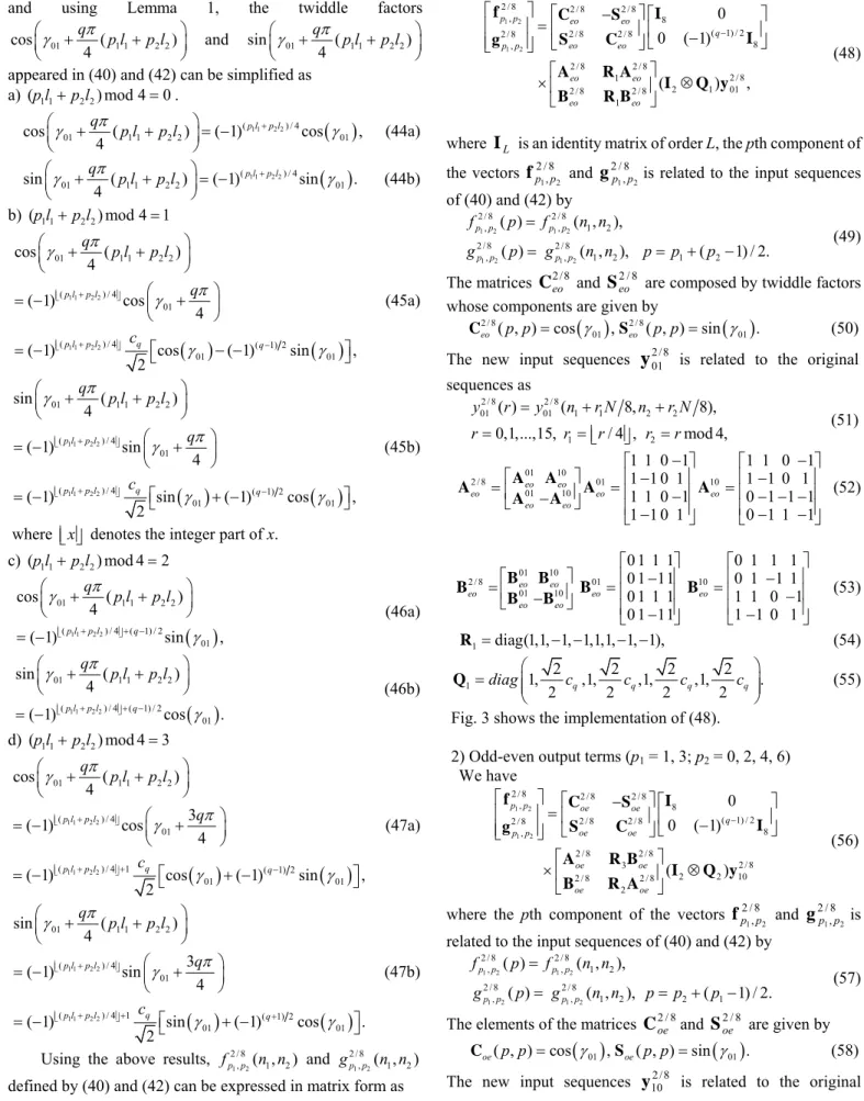
(42)We need to use the following lemma, which was stated in [3].
Lemma 1: Let cos(β(π 4))= 2 2cq and
q
s π
β( 4)) 2 2
sin( = , where β is an odd integer. Then the following is true
i) Forβ=q, =(−1)(q−1)2 q
qs
c .
ii) Forβ 3= q, c3q =−cqands3q =sq. Letting 2 01 1 2 i i i n p N q π γ = =
∑
(43)and using Lemma 1, the twiddle factors 01 1 1 2 2 cos ( ) 4 qπ p l p l γ ⎛ + + ⎞ ⎜ ⎟ ⎝ ⎠ and sin 01 4 ( 1 1 2 2) qπ p l p l γ ⎛ + + ⎞ ⎜ ⎟ ⎝ ⎠
appeared in (40) and (42) can be simplified as a) (p l1 1+p l2 2) mod 4 0= . (1 1 2 2) / 4
( )
01 1 1 2 2 01 cos ( ) ( 1) cos , 4 p l p l q p l p l π γ + γ ⎛ + + ⎞= − ⎜ ⎟ ⎝ ⎠ (44a)( )
1 1 2 2 ( ) / 4 01 1 1 2 2 01 sin ( ) ( 1) sin . 4 p l p l qπ p l p l γ + γ ⎛ + + ⎞= − ⎜ ⎟ ⎝ ⎠ (44b) b) (p l1 1+p l2 2) mod 4 1=( )
( )
1 1 2 2 1 1 2 2 01 1 1 2 2 ( ) / 4 01 ( ) / 4 ( 1) 2 01 01 cos ( ) 4 ( 1) cos 4 ( 1) cos ( 1) sin , 2 p l p l q p l p l q q p l p l q c π γ π γ γ γ + ⎢ ⎥ ⎣ ⎦ + ⎢ ⎥ − ⎣ ⎦ ⎛ + + ⎞ ⎜ ⎟ ⎝ ⎠ ⎛ ⎞ = − ⎜ + ⎟ ⎝ ⎠ ⎡ ⎤ = − ⎣ − − ⎦ (45a)( )
( )
1 1 2 2 1 1 2 2 01 1 1 2 2 ( ) / 4 01 ( ) / 4 ( 1) 2 01 01 sin ( ) 4 ( 1) sin 4 ( 1) sin ( 1) cos , 2 p l p l q p l p l q q p l p l q c π γ π γ γ γ + ⎢ ⎥ ⎣ ⎦ + ⎢ ⎥ − ⎣ ⎦ ⎛ + + ⎞ ⎜ ⎟ ⎝ ⎠ ⎛ ⎞ = − ⎜ + ⎟ ⎝ ⎠ ⎡ ⎤ = − ⎣ + − ⎦ (45b)where ⎢ ⎥⎣ ⎦x denotes the integer part of x. c) (p l1 1+p l2 2) mod 4 2=
( )
1 1 2 2 01 1 1 2 2 ( ) / 4 ( 1) / 2 01 cos ( ) 4 ( 1) p l p l q sin , qπ p l p l γ γ + + − ⎢ ⎥ ⎣ ⎦ ⎛ + + ⎞ ⎜ ⎟ ⎝ ⎠ = − (46a)( )
1 1 2 2 01 1 1 2 2 ( ) / 4 ( 1) / 2 01 sin ( ) 4 ( 1) p l p l q cos . qπ p l p l γ γ + + − ⎢ ⎥ ⎣ ⎦ ⎛ + + ⎞ ⎜ ⎟ ⎝ ⎠ = − (46b) d) (p l1 1+p l2 2) mod 4 3=( )
( )
1 1 2 2 1 1 2 2 01 1 1 2 2 ( ) / 4 01 ( ) / 4 1 ( 1) 2 01 01 cos ( ) 4 3 ( 1) cos 4 ( 1) cos ( 1) sin , 2 p l p l q p l p l q q p l p l q c π γ π γ γ γ + ⎢ ⎥ ⎣ ⎦ + + ⎢ ⎥ − ⎣ ⎦ ⎛ + + ⎞ ⎜ ⎟ ⎝ ⎠ ⎛ ⎞ = − ⎜ + ⎟ ⎝ ⎠ ⎡ ⎤ = − ⎣ + − ⎦ (47a)( )
( )
1 1 2 2 1 1 2 2 01 1 1 2 2 ( ) / 4 01 ( ) / 4 1 ( 1) 2 01 01 sin ( ) 4 3 ( 1) sin 4 ( 1) sin ( 1) cos . 2 p l p l q p l p l q q p l p l q c π γ π γ γ γ + ⎢ ⎥ ⎣ ⎦ + + ⎢ ⎥ + ⎣ ⎦ ⎛ + + ⎞ ⎜ ⎟ ⎝ ⎠ ⎛ ⎞ = − ⎜ + ⎟ ⎝ ⎠ ⎡ ⎤ = − ⎣ + − ⎦ (47b)Using the above results, 2 / 81 2 , ( , )1 2 p p f n n and 2 / 81 2 , ( , )1 2 p p g n n
defined by (40) and (42) can be expressed in matrix form as
1 2 1 2 2 / 8 2 / 8 2 / 8 , 8 ( 1) / 2 2 / 8 2 / 8 2 / 8 8 , 2 / 8 2 / 8 2 / 8 1 2 1 01 2 / 8 2 / 8 1 0 0 ( 1) ( ) , p p eo eo q eo eo p p eo eo eo eo − ⎡ ⎤ ⎡ − ⎤⎡ ⎤ = ⎢ ⎥ ⎢ ⎥ ⎢ ⎥ − ⎢ ⎥ ⎣ ⎦⎣ ⎦ ⎣ ⎦ ⎡ ⎤ ×⎢ ⎥ ⊗ ⎣ ⎦ f C S I I S C g A R A I Q y B R B (48)
where IL is an identity matrix of order L, the pth component of the vectors fp21/,8p2 and g2p1/8,p2is related to the input sequences of (40) and (42) by 1 2 1 2 1 2 1 2 2 / 8 2 / 8 , , 1 2 2 / 8 2 / 8 , , 1 2 1 2 ( ) ( , ), ( ) ( , ), ( 1) / 2. p p p p p p p p f p f n n g p g n n p p p = = = + − (49)
The matrices Ceo2/8 and S2eo/8 are composed by twiddle factors whose components are given by
( )
( )
2 / 8 2 / 8 01 01 ( , ) cos , ( , ) sin . eo p p = γ eo p p = γ C S (50)The new input sequences
y
2 /801 is related to the original sequences as 2 / 8 2 / 8 01 01 1 1 2 2 1 2 ( ) ( 8, 8), 0,1,...,15, / 4 , mod 4, y r y n r N n r N r r r r r = + + = =⎢⎣ ⎥⎦ = (51) 2 / 8 01 10 01 10 01 10 1 1 0 1 1 1 0 1 1 1 0 1 1 1 0 1 1 1 0 1 0 1 1 1 1 1 0 1 0 1 1 1 eo eo eo eo eo eo eo − − ⎡ ⎤ ⎡ ⎤ ⎡ ⎤ ⎢ − ⎥ ⎢ − ⎥ =⎢ ⎥ =⎢ − ⎥ =⎢ − − − ⎥ − ⎣ ⎦ ⎢ ⎥ ⎢ ⎥ − − − ⎣ ⎦ ⎣ ⎦ A A A A A A A (52) 01 10 2 / 8 01 10 01 10 0 1 1 1 0 1 1 1 0 1 11 0 1 1 1 0 1 1 1 1 1 0 1 0 1 11 1 1 0 1 eo eo eo eo eo eo eo ⎡ ⎤ ⎡ ⎤ ⎡ ⎤ ⎢ − ⎥ ⎢ − ⎥ =⎢ ⎥ =⎢ ⎥ =⎢ − ⎥ − ⎣ ⎦ ⎢ ⎥ ⎢ ⎥ − − ⎣ ⎦ ⎣ ⎦ B B B B B B B (53) 1=diag(1,1, 1, 1,1,1, 1, 1),− − − − R (54) 1 2 2 2 2 1, ,1, ,1, ,1, . 2 q 2 q 2 q 2 q diag⎛ c c c c ⎞ = ⎜⎜ ⎟⎟ ⎝ ⎠ Q (55)Fig. 3 shows the implementation of (48).
2) Odd-even output terms (p1 = 1, 3; p2 = 0, 2, 4, 6) We have 1 2 1 2 2 / 8 2 / 8 2 / 8 , 8 ( 1) / 2 2 / 8 2 / 8 2 / 8 8 , 2 / 8 2 / 8 2 / 8 3 2 2 10 2 / 8 2 / 8 2 0 0 ( 1) ( ) p p oe oe q oe oe p p oe oe oe oe − ⎡ ⎤ ⎡ − ⎤⎡ ⎤ = ⎢ ⎥ ⎢ ⎥ ⎢ ⎥ − ⎢ ⎥ ⎣ ⎦⎣ ⎦ ⎣ ⎦ ⎡ ⎤ ×⎢ ⎥ ⊗ ⎣ ⎦ f C S I I S C g A R B I Q y B R A (56)
where the pth component of the vectors fp21/,8p2 and g2p1/,8p2is related to the input sequences of (40) and (42) by
1 2 1 2 1 2 1 2 2 / 8 2 / 8 , , 1 2 2 / 8 2 / 8 , , 1 2 2 1 ( ) ( , ), ( ) ( , ), ( 1) / 2. p p p p p p p p f p f n n g p g n n p p p = = = + − (57)
The elements of the matrices C2oe/8and Soe2/8 are given by
( )
01( )
01( , ) cos , ( , ) sin .
oe p p = γ oe p p = γ
C S (58)
The new input sequences y102/8 is related to the original sequences as
2 / 8 2 / 8 10 10 1 1 2 2 1 2 ( ) ( 8, 8), 0,1,...,15, / 4 , mod 4, y r y n r N n r N r r r r r = + + = =⎢⎣ ⎥⎦ = (59 ) 2 / 8 10 1 2 1 2 1 2 1 2 1 2 ( , ) [ ( , ) ( , / 2)] [ ( / 2, ) ( / 2, / 2)], y n n x n n x n n N x n N n x n N n N = + + − + + + + (60) 01 10 01 10 2 /8 2 /8 01 11
,
01 11,
oe oe oe oe oe oe oe oe oe oe⎡
⎤
⎡
⎤
=
⎢
⎥
=
⎢
⎥
⎣
⎦
⎣
⎦
A
A
B
B
A
B
A
A
B
B
(61) 01 10 11 1 1 1 1 1 1 1 1 1 1 1 1 1 0 1 0 1 1 1 1 1 1 1 1 1 1 1 1 1 1 1 1 1 1 1 1 1 0 1 0 1 1 1 1 1 1 1 1 oe oe oe − − − − ⎡ ⎤ ⎡ ⎤ ⎡ ⎤ − − − − − ⎢ ⎥ ⎢ ⎥ ⎢ ⎥ =⎢ − − ⎥ =⎢ − − ⎥ =⎢− − ⎥ ⎢ − ⎥ ⎢ − − ⎥ ⎢− − ⎥ ⎣ ⎦ ⎣ ⎦ ⎣ ⎦ A A A (62) 01 10 11 0 0 0 0 1 1 1 1 1 1 1 1 0 1 0 1 1 1 1 1 1 1 1 1 0 0 0 0 1 1 1 1 1 1 1 1 0 1 0 1 1 1 1 1 1 1 1 1 oe oe oe ⎡ ⎤ ⎡ ⎤ ⎡ ⎤ − − − − − ⎢ ⎥ ⎢ ⎥ ⎢ ⎥ =⎢ ⎥ =⎢ − − ⎥ =⎢ − − ⎥ ⎢ − ⎥ ⎢ − − ⎥ ⎢ − − ⎥ ⎣ ⎦ ⎣ ⎦ ⎣ ⎦ B B B (63) 2 3 diag(1, 1, 1, 1, 1, 1, 1, 1), diag( 1, 1, 1, 1, 1, 1, 1, 1), = − − − − = − − − − R R (64) 2 2 2 2 2 1, 1, 1, 1, , , , . 2 q 2 q 2 q 2 q diag⎛ c c c c ⎞ = ⎜⎜ ⎟⎟ ⎝ ⎠ Q (65)3) Odd-odd output terms (p1 = –3, –1, 1, 3; p2 = 1, 3) We have 1 2 1 2 2 / 8 2 / 8 2 / 8 , 8 ( 1) / 2 2 / 8 2 / 8 2 / 8 8 , 2 / 8 2 / 8 2 / 8 4 2 3 11 2 / 8 2 / 8 1 0 0 ( 1) ( ) p p oo oo q oo oo p p oo oo oo oo − ⎡ ⎤ ⎡ − ⎤⎡ ⎤ = ⎢ ⎥ ⎢ ⎥ ⎢ ⎥ − ⎢ ⎥ ⎣ ⎦⎣ ⎦ ⎣ ⎦ ⎡ ⎤ ×⎢ ⎥ ⊗ ⎣ ⎦ f C S I I S C g A R B I Q y B R A (66)
where the pth component of the vectors fp21/,8p2andg2p1/,8p2 is related to the input sequences of (40) and (42) by
1 2 1 2 1 2 1 2 2 / 8 2 / 8 , , 1 2 2 / 8 2 / 8 , , 1 2 1 2 ( ) ( , ), ( ) ( , ), ( 3) ( 1) / 2. p p p p p p p p f p f n n g p g n n p p p = = = + + − (67)
The (p, p)th components of the matrices Coo2/8and S2oo/8are respectively given by
( )
01( )
01( , ) cos , ( , ) sin .
oo p p = γ oo p p = γ
C S (68)
The new input sequences y112/8 is defined as
2 / 8 2 / 8 11 11 1 1 2 2 1 2 ( ) ( 8, 8), 0,1,...,15, / 4 , mod 4, y r y n r N n r N r r r r r = + + = =⎢⎣ ⎥⎦ = (69)
(
)
(
) (
)
2/8 11 1 2 1 2 1 2 1 2 1 2 ( , ) ( , ) , / 2 / 2, / 2, / 2 , y n n x n n x n n N x n N n x n N n N =⎡⎣ − + ⎤⎦ −⎡⎣ + − + + ⎤⎦ (70) 01 10 2 / 8 01 10 01 10 1 1 0 1 1 0 1 1 1 1 0 1 1 1 1 0 1 1 0 1 1 1 1 0 1 1 0 1 1 0 1 1 oo oo oo oo oo oo oo − − ⎡ ⎤ ⎡ ⎤ ⎡ ⎤ ⎢ − ⎥ ⎢− − ⎥ =⎢ ⎥ =⎢ − ⎥ =⎢ ⎥ − ⎣ ⎦ ⎢ ⎥ ⎢ ⎥ − − ⎣ ⎦ ⎣ ⎦ A A A A A A A (71) 01 10 2 / 8 01 10 01 10 0 1 1 1 1 1 1 0 0 1 11 1 0 1 1 0 1 1 1 1 0 1 1 0 1 11 1 1 1 0 oo oo oo oo oo oo oo ⎡ ⎤ ⎡ ⎤ ⎡ − ⎤ ⎢ − ⎥ ⎢ − ⎥ =⎢ ⎥ =⎢ ⎥ =⎢ − − ⎥ ⎣ ⎦ ⎢ ⎥ ⎢ ⎥ − − ⎣ ⎦ ⎣ ⎦ B B B B B B B (72) 4=
diag( 1, 1,1,1, 1, 1,1,1),
− −
− −
R
(73) 3 2 2 2 2 1, ,1, , ,1, ,1 . 2 q 2 q 2 q 2 q diag⎛ c c c c ⎞ = ⎜⎜ ⎟⎟ ⎝ ⎠ Q (74)III. COMPUTATIONAL COMPLEXITY AND HARDWARE AREA AND TIME ANALYSIS
In this section, we analyze the performance of the proposed
2-D split-radix-(2×2)/(8×8) algorithm and compare it with some existing algorithms. The analysis and comparison will not only include the arithmetic operations, but also the operations such as data transfers and twiddle factor evaluations since they contribute significantly to the execution time of the algorithm. The analysis of the area and time complexities is also provided. A. Arithmetic complexity
It is assumed that the butterfly computations are implemented by four multiplications and two additions.
1) When N = 2q, from (2) and (3), the number of multiplications and additions is given by
2 2q 2q 4 q q, 2q2q 4 q q 8 .
M × = M × A × = A× + q (75)
2) When N = 4q, the twiddle factors in (17), (22) and (27) become trivial. Therefore
2 4q 4q 2q 2q 12 q q, 4q 4q 2q 2q 12 q q 56 . M × =M × + M × A × =A × + A× + q (76) 3) When N ≥ 8q
a) The computation of the input data sequences 2 / 8 00 ( , ),1 2 y n n 2 / 8 01 ( , )1 2 y n n , 2 / 8 10 ( , )1 2 y n n and 2 / 8 11 ( , )1 2 y n n defined by (33), (39), (60) and (70) requires 2N2 additions.
b) In (47), for each given pair (n1, n2), the matrix ⎥ ⎦ ⎤ ⎢ ⎣ ⎡ 8 / 2 1 8 / 2 8 / 2 1 8 / 2 eo eo eo eo B R B A R A
requires 56 additions since the elements of the matrices are either 1 or –1, so that 7N2/8 additions are needed for 0 ≤ n1, n2 ≤ N/8–1.
c) In equation (48), the computation of the matrix ⎥ ⎦ ⎤ ⎢ ⎣ ⎡ − 8 / 2 8 / 2 8 / 2 8 / 2 eo eo eo eo C S S C
, which is composed by twiddle factors, requires N2/4–A
s additions and N2/2–Ms multiplications,
where As and Ms are the savings from the special cases of
twiddle factors such as 0, ±1, ± 2 2, cos(π/8), sin(π/8), cos(3π/8) and sin(3π/8). Specifically, we can obtain the number of additions and multiplications saved from the special cases of twiddle factors as follows: When p1 = 0 and p2 = 1, 3 for a given value of n1 and 0 ≤ n2 ≤ N/8–1, this case can be taken as an 1-D DHT for the special twiddle factors. The saved number of additions and multiplications can be derived in a way similar to the one presented in [3], they are respectively 6q and 10q. So that the total saved number of additions and multiplications in the case of p1 = 0, p2 = 1, 3, for 0 ≤n1, n2 ≤ N/8–1 is 3qN/4 and 5qN/4. Thus, for all the combination of (p1, p2) in (48), we can obtain As
= 3qN and Ms = 5qN.
d) The computation of the matrix I2⊗Q1requires N2/8 multiplications.
e) The analysis described from (b) to (d) shows that the computation of 2 / 81 2 , ( , )1 2 p p F k k and 2 / 81 2 , ( , )1 2 p p G k k for
even-odd output terms needs 9N2/8–3qN additions and 5N2/8–5qN multiplications. The same number of arithmetic operation is required for odd-even and odd-odd cases. f) The computation of equation (34) requires 3N2/4 additions
for even-odd, odd-even and odd-odd output terms.
From the above discussion, it can be seen that the total number of additions and multiplications involved in the proposed algorithm for N > 8q is as follows
2 / 2 / 2 / 8 / 8 2 / 2 / 2 / 8 / 8 48 49 / 8 9 , 48 15 / 8 15 . N N N N N N N N N N N N A A A N qN M M M N qN × × × × × × = + + − = + + − (77)
For N = 8q, the twiddle factors are given by
2 2 1 2 1 1 2 cos cos , 0 , 1. 4 i i i i i i n p n p n n q N q π π = = ⎛ ⎞ ⎛ ⎞ = ≤ ≤ − ⎜ ⎟ ⎜ ⎟ ⎝ ⎠ ⎝
∑
⎠∑
In thiscase, only (3/8)×(8q)2 =24q2 multiplications are needed in the computation of even-odd, odd-even and odd-odd output terms. Thus, the arithmetic complexity when N = 8q, is given by
2 8 8 4 4 2 8 8 4 4 48 344 , 48 24 . q q q q q q q q q q q q A A A q M M M q × × × × × × = + + = + + (78) The initial values for q = 1 are given by
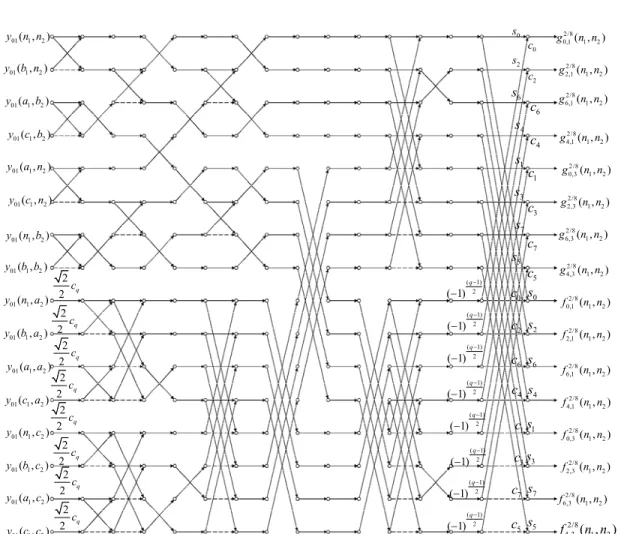
1 1 2 2 4 4 8 8 1 1 2 2 4 4 8 8 0, 8, 64, 384, 0, 0, 0, 24. A A A A M M M M × × × × × × × × = = = = = = = = (79) Similarly, for q = 3 3 3 6 6 12 12 24 24 3 3 6 6 12 12 24 24 47, 260, 1328, 6680, 4, 16, 64, 472. A A A A M M M M × × × × × × × × = = = = = = = = (80)
The flowgraph of length-3×3 DHT is shown in Fig. 4.
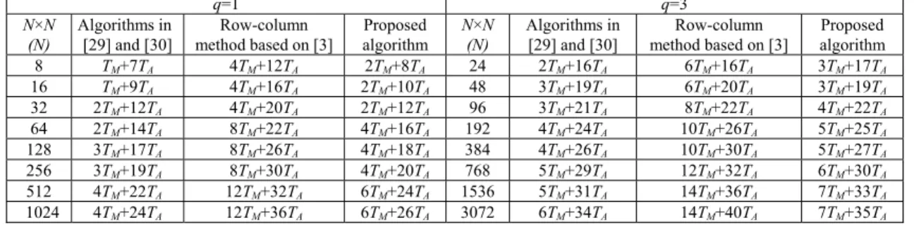
Tables I and II show respectively the arithmetic complexities for q = 1 and q = 3 of the proposed algorithm, the radix-(2×2)/(4×4) algorithms in [29] and [30], and the row-column method based on the 1-D algorithm in [3]. It can be seen from these tables that the proposed algorithm can save almost 10% multiplications and has lower total number of additions and multiplications than that of the algorithms in [29] and [30], and saves about 60% multiplications and 40% additions compared to the row-column method.
B. Data transfers
Based on the fact that the on-chip memory can be accessed faster than external memory (off-chip memory), an appropriate use of the internal registers (on-chip memory) is becoming an important strategy. It is assumed that sufficient registers are available in the processor without using any intermediate transfer operation. The implementation scheme of the proposed algorithm is shown in Fig. 5. The implementation of the butterfly for a given value of n1, n2, consists of reading two points from the external memory of the processor and performing the operations of addition and subtraction using these two points. The result of addition is returned to the external memory whereas that of the subtraction is kept in an internal register. The points kept in the processor are grouped to form y201/8,y102/8 and y112/8 in (48), (56), (66) and to compute the outputs of (48), (56), (66), which are the inputs of the
N/8×N/8 DHT in (40) and (42). The number of data transfers is analyzed as follows:
1) Reading all the input terms x(n1, n2), x(n1, n2+N/2), x(n1+N/2,
n2), and x(n1+N/2, n2+N/2) for 0 ≤n1, n2 ≤ N/2–1from external memory, which requires N2/2 data transfers.
2) Writing 2 / 8 00 ( , )1 2
y n n for 0 ≤ n1, n2 ≤ N/2–1, into external memory to form the input sequences of (32). It needs N2/8 data transfers. 3) Writing 2 / 8 01 ( , )1 2 y n n , 2 / 8 10 ( , )1 2 y n n and 2 / 8 11 ( , )1 2 y n n for 0 ≤
n1, n2 ≤ N/2–1, into the external memory to form the input sequences of forty-eight N/8×N/8 DHTs in (48), (56) and (66). It requires 3N2/8 data transfers.
4) Computation of (37) needs 3N2/4 data transfers.
Thus, the data transfers of the proposed algorithm are given by
2 / 8 2 / 8 2 / 8 2 / 2 / 2 48 / 8 / 8+7 / 4, 8, N N N N N N D × =D × + D × N N > (81) with 2 / 8 2 / 8 2 / 8 1 1 2 2 4 4 2 / 8 2 2 / 8 2 / 8 8 8 4 4 1 1 0, 4, 20, 48 84. D D D D N D D × × × × × × = = = = + + = (82)
Similarly, the data transfers of the radix-(2×2)/(4×4) algorithm in [29] and [30] are given by
2 / 4 2 / 4 2 / 4 2 / 2 / 2 12 / 4 / 4+7 / 4, 8, N N N N N N D × =D × + D × N N≥ (83) with 2 / 4 2 / 4 2 / 4 1 1 0, 2 2 4, 4 4 20. D× = D× = D× = (84) Tables III and IV show respectively the number of data transfers for q = 1 and q = 3 of the different methods for certain value of N. The proposed algorithm leads to a reduction of data transfers over 20% compared to radix-(2×2)/(4×4) algorithm in [29] and [30] and approximately 60% compared to the row-column algorithm.
C. Twiddle factors
It is assumed that the coefficients required by the special butterflies, such as 2 2, cos(π/8) and sin(π/8) are initialized and kept in the internal registers of the processor during the processing time. Firstly, equations (48), (56) and (66) require 3×16× (N/8)×(N/8) =3N2/4 twiddle factors. Secondly, we can obtain the number of twiddle factors for the special cases as follows: When p1 = 0 and p2 = 1, 3, for a given value of n1 and 0 ≤ n2 ≤ N/8–1, the number of the twiddle factors required in this case can be derived in a way similar to the one presented in [3], it is 8q. So that the total number of the twiddle factors for the case where p1 = 0, p2 = 1, 3, for 0 ≤ n1, n2 ≤ N/8–1 is qN. Thus, for all the combinations of (p1, p2) in (48), (56) and (66), the number of the twiddle factors is 12qN. Therefore, the twiddle factors of the proposed algorithm are given by
2 / 8 2 / 8 2 / 8 2 2 2 48 8 8 3 / 4 12 , 8 . N N N N N N TF× =TF × + TF × + N − qN N> q (85) For q = 1, we have 2 /8 2 /8 2/8 2/8 1 1 0 2 2 0 4 4 0 8 8 0 TF× = TF× = TF× = TF× = . (86) For q = 3, we have 2 /8 2 /8 2/8 2/8 3 3 0 6 6 0 12 12 0 24 24 0 TF× = TF× = TF × = TF × = . (87)
Analyzing the twiddle factors required in the radix-(2×2)/(4×4) algorithm in [29] in a similar way, we have
2 / 4 2 / 4 2 / 4 2
2 2 12 4 4 3 / 4 6 , 4 .
N N N N N N
For q = 1 2 /8 2/8 2 /8 1 1 0 2 2 0 4 4 0. TF× = TF× = TF× = (89) For q = 3 2 /8 2 /8 2 /8 3 3 0 6 6 0 12 12 0. TF× = TF× = TF × = (90)
Tables V and VI show respectively the comparison of twiddle factors for q = 1 and q = 3 for different methods. It can be seen that, in most cases, our algorithm saves approximately 35% compared to the algorithm in [29] and [30], and approximately 40% compared to the row-column method. D. Area complexity and time complexity analysis
In this subsection, we compare the area complexity and time complexity of the proposed split-radix-(2×2)/(8×8) algorithm with the split-radix-(2×2)/(4×4) algorithm presented in [29] and the row-column method using [3] based on single multipliers, multiplier/accumulators and butterfly processors. The algorithm presented in [30] has the same area and time complexity as that of [29].
1) Systems Using Multiplier or Multiplier/Accumulator Primitives
As described in [9], in systems using software in conjunction with a hardware adder to accomplish multiplications, such as general-purpose microcomputers without coprocessors, the computation time of the algorithm is determined primarily by the number of multiplications. In systems using a single hardware multiplier, such as DSP microcomputers, both multiplies and additions contribute heavily in determining the run time. In both cases, the area complexity (the area of one multiplier or multiplier/accumulator) of three algorithms is the same. Therefore, the area-time complexity is determined by the computational time. As can be seen from Tables I and II, the proposed split-radix-(2×2)/(8×8) is clearly preferable to the split-radix-(2×2)/(4×4) presented in [29] and row-column method based on [3] in terms of computational time.
2) Multiprocessor Implementations Based on Butterflies In this subsection, for simplicity, we implement strictly the algorithms according to the flowgraph. That is to say, we dedicate one multiplier (or one adder) to implement one multiplicative (or additive) operation. Let TM and TA be
respectively the computational time of one multiplication and one addition. The designed modules of the three algorithms are described as follows.
a) Implementation of the split-radix-(2×2)/(8×8) algorithm with 5 modules
The first module is used to implement (33), (39), (60) and (70) to obtain 2 / 8 00 ( , ),1 2 y n n 2 / 8 01 ( , ),1 2 y n n 2 / 8 10 ( , )1 2 y n n and 2 / 8 11 ( , )1 2
y n n for 0 ≤ n1, n2 ≤ N/2–1. We design the butterfly shown in Fig. 1 as type-I butterfly, which consists of four radix-2 butterflies. Totally, (N×N)/4 type-I butterflies are required. The computational time of the first module is 2TA.
The second module is designed to obtain the even-even output terms, that is, to implement one (N/2)×(N/2) DHT. The computational time of the second module is TN2/8/ 2×N/ 2.
The third module is used to obtain the even-odd output terms, including (48) and 16 parallel (N/8)×(N/8) DHTs and one third data processing of (37). We divide further this module into 3 smaller modules. The module 3-1 is used to implement (48). We design the butterfly shown in Fig. 3 as the type-II butterfly, which can be decomposed into five stages. The first stage consists of four radix-2 butterflies and four modified multiplier-adder butterflies. The second stage, the third stage and the fourth stage consist of six, six and eight radix-2 butterflies, respectively. The last stage consists of eight multiplier-adder butterflies. Note that for the last stage, we assume that some special twiddle factors, such as 2 2 , cos(π/8) and sin(π/8), are implemented by the special butterflies. Therefore, (N/8)×(N/8) type-III butterflies are required. The computational time is 2TM+5TA. The module 3-2
is used to implement 16 parallel (N/8)×(N/8) DHTs. The computational time is TN2/8/8×N/8. The module 3-3 is used to implement one third data of (37). This module is implemented by 8×(N/8)×(N/8) radix-2 butterflies. The computational time is TA. Totally, The computational time of the third module is
2/8 / 2 / 2 2TM +5TA+TN ×N +TA.
The fourth module is used to obtain the odd-even output terms, including (56) and 16 parallel (N/8)×(N/8) DHTs and one third data processing of (37).
The fifth module is used to obtain the odd-odd output terms, including (66) and 16 parallel (N/8)×(N/8) DHTs and one third data processing of (37).
The design of the fourth and the fifth module is similar to the third one. We assume that when the first module is finished, the second module, the third module, the fourth module and the fifth module are working in parallel. Under this assumption, the total computational time for the proposed algorithm is given by
{
}
2/8 2/8 2/8 / 2 / 2 /8 /8 2 max ,2 6 . N N A N N M A N N T × = T + T × T + T +T × (91)For q = 1, the initial values of (91) are 2/8 2 2 2/8 2/8 4 4 2 2 2 , 2 4 . A A A T T T T T T × × × = = + = (92) For q = 3, as can be seen in Fig. 4, the initial values of (91) are 2/8 3 3 2/8 2/8 6 6 3 3 2/8 2/8 12 12 3 3 9 , 2 11 5 2 14 . M A A M A M A M A T T T T T T T T T T T T T T × × × × × = + = + = + = + + = + (93) Substituting the above initial values into TN2/8/ 2×N/ 2 and
2 /8 /8 /8
2TM +6TA+TN ×N , we find that the former is always smaller than the latter. Thus, (91) becomes
2 /8 2/8
/8 /8
2 8 .
N N M A N N
T × = T + T +T × (94) Since the multiplication by (1/2) in Fig. 4 is simply a right-shift operation, hence, the computational time is not taken into account in this analysis.
b) Implementation of the split-radix-(2×2)/(4×4) algorithm with 5 modules
The first module is used to implement (6), (12), (26) and (31) to obtain 2 / 4 00 ( , ),1 2 y n n 2 / 4 01 ( , ),1 2 y n n 2 / 4 10 ( , ),1 2 y n n and 2 / 4 11 ( , )1 2
y n n for 0 ≤ n1, n2 ≤ N/2–1. The computational time is 2TA.
The second module is used to obtain the even-even output terms. The computational time is TN2/ 4/ 2×N/ 2.
The third module is used to obtain the even-odd output terms, including (17), 4 parallel (N/4)×(N/4) DHTs and one third data processing of (10). The implementation is similar to that of the split-radix-(2×2)/(8×8) algorithm. The computational time of the third module is TM +2TA+TN2/ 4/ 2×N/ 2+TA.
The fourth module and the fifth module are used to obtain the odd-even and odd-odd output terms, respectively. Their design is similar to the third module.
The total computational time for the split-radix-(2×2)/(4×4) algorithm in [29] is given by
{
}
2 / 4 2/ 4 2/ 4 / 2 / 2 / 4 / 4 2 / 4 / 4 / 4 2 max , 3 5 N N A N N M A N N M A N N T T T T T T T T T × × × × = + + + = + + (95)The initial values of (95) for q = 1 and q = 3 are the same as those of (92) and (93).
c) Implementation of the row-column method
Using the similar implemental scheme as the aforementioned two algorithms, we can easily obtain the computational time for the 1-D split-radix-2/8 DHT algorithm [3] as follows:
{
}
2/8 2/8 2 /8 / 2 /8 2 max ,2 3 N A N M A N T = T + T T + T +T (96) For q = 1, the initial values of (96) are2/8 2 2/8 2/8 4 2 , 2 . A A A T T T T T T = = + = (97) For q = 3, the initial values of (96) are
2/8 3 2/8 2/8 6 3 2/8 2 /8 12 3 2 , 3 , 3 2 5 . M A A M A M A M A T T T T T T T T T T T T T T = + = + = + = + + = + (98) Therefore, the total computational time for the row-column method is given by:
{
}
2/8 2/8 2/8 / 2 /8 2 2 6 2max , 2 3 RC N A N A N M A N T T T T T T T T = + = + + + (99)The initial values of (99) for q = 1 and q = 3 are the same as those of (97) and (98).
Table VII shows the comparison of computational time for q = 1 and q = 3. As can be seen from this table, the proposed algorithm requires less computational time than row-column method based on [3] but a little more computational time than that of the algorithm in [29] and [30]. The additional time complexity will be discussed in the following.
When using the parallel implementation structure described above, the required multipliers and adders are the same as the number of multiplications and additions given in Tables I and II. Therefore, the area complexity can be directly evaluated from these two tables. It can be seen that the proposed algorithm
requires less area complexity than that of the algorithm presented in [29] and [30] and the row-column method based on [3].
As a conclusion of this section, we explain why the proposed algorithm achieves the above attractive results (reductions in arithmetic complexity, data transfers and twiddle factors) compared to the algorithms in [29] and [30]. There are mainly three reasons. Firstly, the pair of special angles (π/8) and (3π/8), just like the 1-D split-radix-2/8 algorithm in [3], is taken into consideration in the proposed algorithm to reduce both the arithmetic complexity and the twiddle factors. However, these cases have not been considered in [29] and [30]. Secondly, the proposed approach, decomposing an N×N DHT into one N/2×N/2 DHT and forty-eight N/8×N/8 DHTs, can save the data transfer. Meanwhile, the new scheme decreases the number of multiplications at the cost of a little more additions, as can be seen in Tables I and II. Finally, the computation process is recursive, the savings in arithmetic complexity, data transfers and twiddle factors of initial values (or relative smaller transform length) are accumulated with the increases of the value of transform length N. However, for the hardware time complexity analysis, the additional time complexity of the proposed algorithm is mainly caused by the spread of cosine and sine functions in (40) and (42). This can be observed from the first stage of Fig. 3. When implementing the proposed algorithm, we have to dedicate an additional group of multipliers compared to the algorithm in [29] and [30].
IV. SOFTWARE IMPLEMENTATION OF THE PROPOSED AND SOME EXISTING 2-DDHT ALGORITHMS
In this section, just like [43], we compare the proposed algorithm with some existing algorithms for the 2-D DHT in terms of computer run times, which include fetch instruction time, decoding time and write back time. These algorithms have been implemented with “C” programming language and carried out on a PC machine, which has an Intel Core2 Duo CPU with speed of 2200MHz and 3072 MB RAM. The run-time of these algorithms has been calculated using Visual C++ (VC++) Version (9).
A. Comparison of the proposed algorithm with some existing 2-D DHT algorithms in terms of computer run times We compare the proposed algorithm with the algorithms presented in [29] and [30] and the row-column method based on [3] in terms of computer run-times. Tables VIII and IX show respectively the run times required in these algorithms for q = 1 and q = 3. The times in Table VIII and IX represent the average obtained by repeating the execution of the algorithm. As it can be seen from these tables, the proposed algorithm approximately saves average 11% compared to the algorithms in [29] and [30] and 60% compared to the row-column method based on [3]. Since we use the recursive structure to implement the algorithms, the C codes are still far from optimal and there is much room for performance improvement.
B. Comparison of the proposed algorithm with some existing 2-D DHT algorithms in terms of the image compression
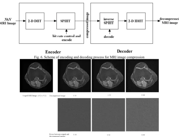
![Table I Comparison of Arithmetic Complexities for q = 1 (Saving denotes the saving of arithmetic complexity compared to the algorithm in [29] and [30])](https://thumb-eu.123doks.com/thumbv2/123doknet/14530221.533420/15.918.59.862.93.254/comparison-arithmetic-complexities-saving-arithmetic-complexity-compared-algorithm.webp)