Convex set estimation from support line measurements and applications to target reconstruction from laser radar data

Room 14-0551

77 Massachusetts Avenue Cambridge, MA 02139

MITLibraries

Document Services

http://libraries. mit. edu/docs

DISCLAIMER OF QUALITY

Due to

the condition

of the original material, there are unavoidable

flaws in this reproduction. We have made every effort possible to

provide you with the best copy available. If you are dissatisfied with

this product and find it unusable, please contact Document Services as

soon as possible.

Thank you.

Due to the poor quality of the

original document,

there is

November 1990 LIDS-P-2005

Convex Set Estimation from Support Line Measurements

and Applications to Target Reconstruction from Laser Radar Data*

A.S. Lelel

S.R. Kulkarni"

A.S. Willsky

'Massachusetts Institute of Technology

Lincoln Laboratory

244 Wood Street

Lexington, Massachusetts 02173

2

_{Massachusetts Institute of Technology}

Center for Intelligent Control Systems and

Laboratory for Information and Decision Systems

77 Massachusetts Avenue

Cambridge, MA 02139

Abstract

This paper addresses techniques of convex set estimation from support line measurements and introduces the application of these methods to laser radar data. The algorithms developed *This research was conducted at. M.I.T. Lincoln Laboratory. sponsored by the Department. of the Navy undler Air Force contract. F19628-90-C-0002. andi at. M.I.T. ttuller U.S. Artilv Research Oflice contract l)AAI,(3-8;-1\--.)171 anli National Science Founldation contract. ECS-8700903.

utilize varying degrees of prior information. Quantitative assessments of their performance with respect to various parameters are provided. As expected, prior information as to object shape and orientation greatly improves performance. Interestingly, nearly the same performance is obtained with and without using the prior information about object orientation, enabling us to extract an estimate of orientation.

These convex set estimation techniques are applied to the problem of target reconstruction from range-resolved and Doppler-resolved laser radar data. The resulting reconstructions pro-vide size and shape estimates of the targets under observation. While such information can be obtained by other means (e.g. from reconstructed images using tomography), the present meth-ods yield this information more directly. Furthermore, estimates obtained using these methmeth-ods are more robust to noisy and/or sparse measurement data and are much more robust to data suffering from registration errors. Finally, the present methods are used to improve tomographic images in the presence of registration errors.

1. INTRODUCTION

In this paper, we develop techniques for estimating convex sets from support line measurements and introduce the application of these methods to target reconstruction from resolved laser radar measurements. A support line of a two-dimensional convex set refers to any line which just grazes the boundary of the set, so that the set lies entirely in one of the halfplanes defined by the support line. Clearly, a convex set is completely determined by its support lines at all orientations, and can be obtained by simply intersecting the corresponding halfplanes. From a finite number of support lines an approximation to the convex set may be obtained in the same manner. However, any physical measurements giving rise to support lines are in general noisy, and simply intersecting the halfplanes may not yield satisfactory results. Prince and Willsky [1, 2] formulated the problem of estimating a convex set from noisy support line measurements and studied a variety of algorithms.

(Greschak [3], Stark and Peng [4], and others have done related work.)

Here, we introduce three new estimation algorithms which utilize varying degrees of prior infor-mation. The first is simply an extension of an algorithm from [1, 2], which allows the measurements to be spaced nonuniformly in angle. The reconstructed polygon has sides at the measurement an-gles. The second algorithm allows the reconstruction angles to be specified independently of the measurement angles. This corresponds to the incorporation of prior information concerning the shape of the object, in that the reconstruction is the best N-gon with sides at fixed angles fitting the measurements. The final algorithm is similar to the second algorithm except that rotation of the constellation of reconstruction angles is allowed. Hence, this algorithm provides both an N-gon reconstruction as well as an orientation estimate.

There are a number of applications in which support line information can be extracted from physical measurements of an object. For example, in tomographic imaging the nonzero extent of each transmission projection provides support information of the underlying mass distribution

[1, 2]. Another possible application arises in tactile sensing, in which the support information can be obtained by a robot jaw repeatedly grasping an object [1, 2]. In these applications, convex set estimation algorithms can be used to provide reconstructions of the object, either independently or in conjunction with other algorithms.

An application introduced and studied in this paper is that of target reconstruction from laser radar data. Resolved laser radar measurements of a target provide information as to the extent of the target in space. For example, a range-resolved measurement indicates where the target begins in range along the radar line of sight (LOS). If a plane is drawn at this range perpendicular to the line of sight, the target lies completely to one side of this plane and in fact is just grazed by this plane. Range-resolved measurements from a number of aspects yield a set of support planes of the target which could conceivably be used to obtain a three-dimensional estimate of the target. In this paper, we restrict attention to the case in which all the aspects, i.e. LOS's, lie in a plane, so that the problem is reduced to two dimensions. In a similar manner, Doppler-resolved measurements of a spinning target contain support plane information, which reduces to support line information under the restriction that all aspects lie in a plane.

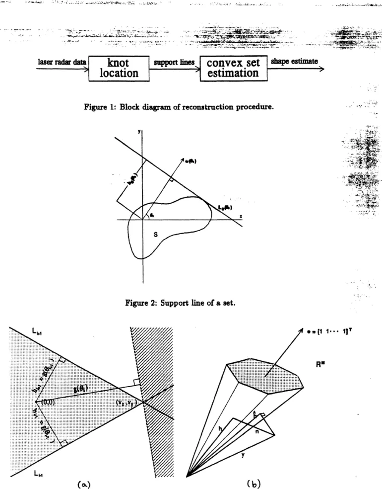
The basic reconstruction procedure of this paper may be decomposed in the manner indicated by Figure 1. In the first module, support line information is extracted from the laser radar data using an estimation procedure developed by others [5, 6] for the location of knots in spline approximations. The support line measurements obtained are in general noisy for various reasons. In the second module, the convex set estimation techniques developed in this paper provide an estimate of the target given these noisy support line measurements and prior knowledge as to target shape.

Section 2 provides the background, formulation, and basic approach to the estimation problem. The three specific estimators are presented in Section 3, along with an assessment of their perfor-mnance. In Section 4, we describe the laser radar data, the way in which the data contain support

line information, and the technique used to extract this information. The reconstruction algorithms are applied in Section 5 to range-resolved measurements and Doppler-resolved measurements ob-tained through simulated, laboratory, and field measurements. Reconstructions obob-tained by using the present methods are compared with reconstructed images produced by standard tomographic methods [7]. Also, a a method is introduced whereby the tomographic reconstructions from unreg-istered data may be greatly improved using our reconstruction algorithm as a preprocessor of the data. Finally, in Section 6 our results are summarized and possible directions for further work are suggested.

2. CONVEX SET ESTIMATION FROM SUPPORT LINE MEASUREMENTS

In this section we first discuss the ideas of support lines and support functions of convex sets. Although the exact support values at all angles characterize a convex set, in many applications only a finite number of noisy measurements are available. Accordingly, we formulate and discuss the basic approach to the problem of estimating a convex set from such measurements.

2.1 Background and Definitions

Using a coordinate frame fixed with respect to the set, we define the support line of the set S at angle ₀O (denoted by Ls( 0o)) to be the line orthogonal to the vector w(Oo) = [cos 0O sin o]T that 'just grazes' the set (see Figure 2). The support value hs(0o) is defined as the maximum projection onto w(0o) of all points in S:

hs(Oo) = sup sTw(O), 0 (1)

sES

and its magnitude, Ihs(Go)l, is the minimum distance from LS(9o) to the origin. In fact, since all points on Ls(Oo) have the same projection onto w(Go)-namely, the support value hs(0o)-the support line may be expressed precisely as

Ls(6o) =

{X

From all of this, it follows that the set S lies in a particular one of the two halfplanes defined by

Ls(8o).

We will refer to hs(O) as the support function of the set S. This function is continuous and periodic with period 27r. Sampling the support function at a finite number of angles O1, 2,... , OM

yields a support vector hs = [hs(61) hs(62) ... hs(OM)]T. Also, from Figure 2, it should be apparent that support lines provide no information as to concavities in the set, so that support lines at all orientations determine only the convex hull of the set. In fact, the support function of a set uniquely determines the set iff the set is convex. For this reason, we restrict attention to convex sets in subsequent discussion unless otherwise stated.

Note further that if the support function of a set is known for only a finite number of angles, the set is not uniquely determined, since an entire equivalence class of sets shares the same support vector. In this paper, the set that we associate with any given support vector is the polygonal set bounded by the support lines, which is, of course, the largest set in the equivalence class.

Although every convex set has a support function defined on [0, 27r) that uniquely determines it, not every function defined on this domain is the support function of some set. Naturally, the same is true of support vectors. A number of necessary and sufficient conditions for a function to be a valid support function have been developed [8, 9, 10, 11, 12]. In this paper, we will be using a version of the following condition suitable for support vectors: A twice-differentiable function h(O) is a valid support function iff h"(9) + h(O) > 0 (for example, see [11]). Roughly, the reasoning behind this condition is that for convex objects, the curvature of the boundary is given by K(O) = h"(9) + h(O) and may never be negative.

The derivations of several of the results to be described in subsequent chapters are facilitated by considering the support function of a set, rather than its support vector. In this continuous-angle framework, support functions possess several useful properties which reduce in a natural way to corresponding properties for support vectors. The set S1 consisting of a single point located on the z-axis at (zo, 0) has support function hs, (0) = zo cos

8.

[9] where D denotes the Minkowski set sum defined by A E B = {a + bla E A,b E B}, we have that the support function of a point (zo, yo) is given by h(8) = zo cose + yo sinG. Now, by representing a polygon Sp as the convex hull of its vertices (zi, yi) and from the property that [9] hcov(AuB) = max(hA, hB) we find that the support function of a polygon is given by

hsp (8) = max(zxi cos

8

angles of the faces which intersect to form the ith vertex, we may rewrite the support function of a

polygon as hs, (8) = xi cos

8

8

_8i]

form that hsP (8) takes.

2.2 Formulation and Basic Approach

We model our support measurements Y1, Y2,..., YM at measurement angles 8

1, 02,..., OM as

consisting of the true support values of the set hi = h(8i) corrupted by noise. That is, yi = hi + ni for i = 1, 2,.. ., M where the {ni} are samples from some noise distribution. We emphasize that by noisy measurements we mean uncertainty in the support values and not in the measurement angles. The measured support values yi constitute the elements of what we refer to as the measured support vector y.

gave rise to them and, in fact, may not correspond to any set. We adopt the approach introduced in [1, 2] for estimating a convex set by finding the valid support vector h that is closest in some sense to y. A natural choice is to minimize Euclidean distance in support vector space. This choice results in an estimation problem for which there exist efficient computational algorithms.

As previously mentioned, there are many convex sets sharing the same (valid) estimated support vector h. The particular convex set that we associate with h is the polygon bounded by the support lines corresponding to h. Since we are more directly interested in minimizing some measure of distance in object space, we evaluate the quality of our reconstructions by using a quantitative measure of the error between the true object S and its reconstruction S. The measure of error we use here is the area of their symmetric difference SAS = (s u S) \ (s n S).

The idea of choosing h as the valid support vector closest to y can be given a nice geometric interpretation [1, 2]. Specifically, the set of valid M-dimensional support vectors forms a cone C in RM, and the estimation procedure can be regarded as projecting the measurement vector y onto C (see Figure 3b). To carry out this projection, a characterization of the support cone is required. Prince and Willsky gave such a characterization by proving a necessary and sufficient condition for a vector h to be a valid support vector in the case of uniformly spaced measurement angles. Our estimators require an extension of this consistency condition to the case of angles which are in general nonuniformly-spaced. This condition is a discrete version of the consistency condition h"(0) + h(O) > 0 for twice-differentiable support functions. In fact, the discrete version can be obtained by using the trigonometric spline form of support function of a polygon and interpreting the derivatives in a distributional sense. The discrete condition can also be obtained from a geometric approach as in Figure 3a. Given support lines Li-1 and Li+l at Oi-I and 0i+l,

a third support line at Oi is consistent only if it lies to the left of the intersection point of Li-1 and Li+1. Together with sufficiency as shown in [1, 2], this leads to the consistency condition for

a triplet of support values at adjacent and in general nonuniformly-spaced angles, given by [13]:

hi-1 sin(8i+l --Oi) - hi sin(8i+l -

Oi-1)

8i-1)

0.

Enforcing this inequality for all adjacent triplets yields a necessary and sufficient condition for a vector to be a valid support vector. Namely,

Ch > 0 (4)

where

- sin(08 -O M) sin(8l - OM) o 0 sin(8₂ - 81)

sin(8₃ - 82) - sin(8₃ - 81) sin(82 - 81) 0 o

C = o0 sin(8₄ - 83) - sin(9₄ - 82) sin(6, - 82) 0 (5)

sin(6M - 8M1 ) 0 0 sin(l8 - 8M) - sin(l -- M-1 )

With such a consistency condition, we can formulate several estimation algorithms which are dis-cussed in the next section.

3. ESTIMATION ALGORITHMS

The estimation algorithms that we present in the following three sections arise from increasingly general formulations of the problem of obtaining polygonal shape estimates from noisy support measurements. The most specific case was considered by Prince and Willsky [1, 2], in which a polygon with faces at a fixed number of uniformly-spaced measurement angles is estimated. A generalization of this algorithm results in relaxing the assumption of uniform spacing. A third formulation consists of estimating a polygon with faces at a set of prespecified reconstruction angles that are not necessarily the same as the set of of measurement angles. Both sets of angles are

nonuniformly-spaced, in general. Fourth, we might allow rotations of the prespecified constellation of reconstruction angles in order to obtain joint orientation and shape estimates of objects. The following subsections treat the three generalizations.

3.1 Reconstruction with sides at the measurement angles

In this problem, we have a finite set of noisy support measurements {Yx, Y2,..., YM} at angles 01 < 02 < ... < 8M. We wish to reconstruct a convex polygon, or equivalently the valid support vector h, with sides at the measurement angles, that is closest to the measurement vector y. The solution is obtained by solving

M

h

argminch>

E(Yi - hi)

(6)

i=1

where C is given by (5). We refer to this estimator as EUA, an acronym for Nonuniform Angles, since the present algorithm is an extension of one developed by Prince and Willsky for uniformly-spaced angles. Since the cost function is quadratic and the constraints are linear, the solution to this problem can be obtained using standard quadratic programming techniques [14, 15]. We note that

NUA, as well as the algorithms of the following subsections result in biased estimators (see Appendix

A).

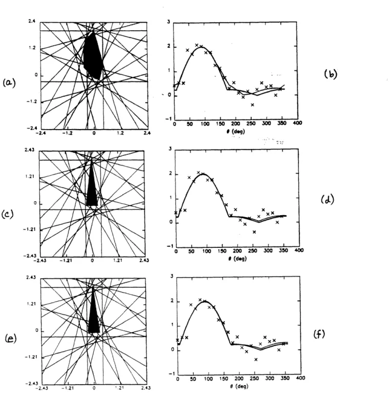
To illustrate the behavior of NUA, we consider the following example. The original object used in this example is an isosceles triangle with vertices at (2,0), (-0.25, 0), and (0.25, 0). We use this triangle throughout the paper and refer to it as the 'standard triangle.' The data consist of M = 24 uniformly-spaced noisy measurements (a = 0.25). Figures 4a,b depict the results in both object space and support function space using the estimator NUA. Figure 4a shows the bold outline of the true object (the standard triangle), the noisy support lines, and the shaded polygonal reconstruction produced by NUA. Correspondingly, Figure 4b shows the support function h(8) of the true object, the noisy support values (yi}, and the support function h(8) of the estimated object.

The quantitative measure of reconstruction error that we use throughout the paper consists of the area of the symmetric difference between the reconstructed object and the true object, normalized by the area of the true object. This error is denoted by E, and for the present example has the value E = 1.56.

3.2 Best N-gon fitting M measurements with fixed reconstruction angles

In this section, we exploit prior information as to the angles of the object's sides, in order to obtain reconstructions of higher quality than those we expect to obtain using 11U1, which utilizes no prior information. Specifically, we consider the problem of determining the N-sided polygon with prespecified face angles that best fits a set of noisy support values at M measurement angles. For example, one might wish to reconstruct the best equilateral triangle given a set of, say, twenty noisy measurements of an object known a priori to be triangular.

In formulating this problem, we let {81,02,..-.,M}, {Y,Y2,...,YM}, and {(1, 02,. .. ,4N}

de-note the M measurement angles, the measured support values at these angles, and the N recon-struction angles, respectively. Given these quantities, we wish to estimate an N-gon specified by the consistent set of support values {hb(l ), h,(q2), ... , ho(vN)} at the specified N-gon face angles which minimizes

M

J(ho,(l 1), h,(0 2), **.., h.(qN)) = (h>(oi) - yi)2, (7)

i=1

where h(O6i) denotes the value at Oi of the support function hk(.) of our estimated N-gon (see (8) and the associated explanation). Eq. (7) corresponds to finding a set of support values (i.e. finding

h,(cbi) for all i) at the reconstruction angles that minimizes the sum of the squared deviations

between the measured support values and the values of the piecewise sinusoidal support function of the reconstructed polygon at the measurement angles.

Let qLj and OR, denote the reconstruction angles immediately to the left and right of the ith measurement angle 0i, and let hLi and hRi denote the corresponding reconstructed support values. Since the support function of a polygon is piecewise sinusoidal with cusps at the face angles, we can obtain the entire support function from its values at the face angles by simply determining the appropriate sinusoid in each interval. That is, the support function of the reconstructed object evaluated at Oi is given by

sin(,Ri - Oi) sin(i - Li) h

h+(8;) = .hL; + -hR, (8)

sin(qRi - qLi) sin(qRi - qLi )

From (7) and (8), our problem is formulated as

h+(q$₁)

h = = argminch,>0(AhO - y)TAh4,, (9)

where y

l Y2

is the measurement vector, C is the consistency matrix of (5)

and sin(R, -OLti ) corresponding to the reconstruction angles qLi and ksRi on either side of Oi.

We refer to the estimator of (9) as BNGON. As before, since the cost function in (9) is quadratic in the reconstructed support values and the consistency constraint is linear, the problem can be solved by QP techniques. Incidentally, under certain conditions there may be nonunique solutions. However, this is not the generic case, and we refer the reader to Appendix B and [13] for more details.

An example of BNGON, similar to that discussed in Section 3.1, is shown in Figure 4c,d. The example consists of reconstructing the best triangle with reconstruction angles at 7.125°, 82.875°, and 270° equal to those of the standard triangle, given M = 24 uniformly-spaced noisy (a = 0.25) support measurements. The pictures in both object space and support function space are shown, with the reconstructed object incurring an error of E = 0.17 with respect to the true object.

The BNGON reconstruction in the figure originates from the same set of measurements as the NUA reconstruction in the same figure (i.e., the same noise realization was used), allowing comparison of the two. Visually, it is clear that the prior information that the true object is a triangle with known face angles allows BNGON to outperform NUA. This is also seen quantitatively by noting that

EBNGON = 0.17 while ENVI = 1.56. However, prior information as to the number of faces and the face angles of the true object may not be known precisely, and in this case one would expect some degradation in performance. Nevertheless, as we will see in Section 3.4, BNGON still outperforms

NUA even in the presence of a broad range of errors in the prior information. Furthermore, one

important source of errors leads to a natural generalization of the BNGON algorithm. Specifically, while in many cases it may be reasonable to assume that one has prior information about number of faces and their relative angles, one would typically not expect to have prior information on the absolute orientation of the object. In the next subsection we describe a generalization of BNGON

that addresses this problem.

3.3 Best N-gon with fixed relative spacing of reconstruction angles

In this subsection, we assume somewhat less prior information than in BNGON by formulating a problem in which the relative (rather than the absolute) angles of the object's sides are known. Specifically, let {81, 02,..., OM} and {Y(81), Y(02),..., Y(OM)} denote the M measurement angles and the measured support values at these angles, as before. However, unlike before, the

recon-struction angles are given by (1{ + a, 02 + a,...,O N + a}, where {q1, 02, , ... N} are known

and a E [0, 27r) serves as an unknown offset parameter fixing the absolute locations of the re-construction angles. Essentially, we wish to minimize the cost function in (9), with the excep-tion that the estimator here is free to rotate the constellaexcep-tion of reconstrucexcep-tion angles in order to achieve minimum cost in the estimate. That is, we wish to jointly estimate values of a and

({ho(l + a), ho(02 + a),..., hk(bN + a)} that minimize

M

J(,a, hk(ol + a), h.(q 2 + a),..., hb(,N + a)) =

E(h(ei)

where ho(Gi), using (8), is given by

h,(i) = sin(qRi + a - 0i) h + sin(/i - L - a)h (11)

sin( R, - OL, ) sin(R - L, )

and the {hO(Oi + a)} are constrained to be a set of consistent support values.

Note that while the criterion (10) is quadratic in the values of hk at the reconstruction angles 01 + a,... , ON + a, it is certainly not quadratic in a (see (11)). Thus, the minimization of (11) is not a simple quadratic programming problem. Nevertheless the structure of this criterion does allow us to obtain a reasonably efficient QP-based optimization algorithm, which we refer to as BNGONROT. Specifically, let Jh (a) denote the cost resulting from a best choice of support vector for

a fixed value of a:

Jh,(a) = min J(a, h0(l 1 + a), h0(02 + a),..., hk(OQN + a)) (12)

Note that solving (12) for any given value of a is simply a BNGON problem solved via a QP computation as described previously. Note also that the minimization of (10) corresponds to choosing a to minimize Jh,(a). Thus a brute force approach to minimizing (10) is to perfrom an

exhaustive search over the values of Jh,(a), where each evaluation of this function involves a QP computation. Our more efficient method involves a gradient-like search for the optimum value of a. However, the nature of the problem is such that there are two important distinctions between our algorithm and a standard gradient descent algorithm. First of all, note that

Jh,(a) = J(a, h;(l1 + a), h*;(*2 + a),,h(N + a)) (13)

where h;(Oi + a), i = 1,..., N are the optimal values of the reconstructed support vector for the given value of a. Thus,

dJh,(a)

OJ

+a)

da -- +

_{.i=, 0h~(i + )}

_Ha

The difficulty here is that computing the sensitivity of the optimal support values h;(Oi + a) with respect to a is not easily obtained (since a QP optimization is involved). Thus, instead of (14), we simply use

ot (a, h; ( 1l + a), h*(0 2 + a),..., h(N + )) = 2 Oh() (h() - y()) (15)

(( ())=l ()

where h¢,(0i) is obtained from (11) with the hLi, hR, values corresponding to the h*(i + a), and

0hj(0j) _ cos(Ri + a - )h _ cos(i - Li - a)h (16)

Oa sin(_Ri - - Li) sin((R- - ,Li)

The second key point is that Jh,(a) is, in general, a highly nonconvex function of a (see [13] for examples and discussion). Thus it is necessary to determine all of the local minima of Jh,(a) and choose the one with lowest cost. Since a is a scalar, constrained to lie between 0° _{and 360}°_, we can do this in the following manner.

We begin at a = 00 and solve the QP problem of (9). Using the estimated support values, we compute (14) and perform a gradient ascent or descent step depending on whether its sign is positive or negative, to obtain a new value of a. We are then committed to performing gradient ascent until we reach the first maximum or gradient descent until we reach the first minimum. We then perform the following steps repeatedly: (1) solve (9), (2) compute the gradient, and (3) perform a gradient step. Once an appropriate convergence criterion has been met (as discussed below), indicating that a local minimum or maximum has been found, we store this value of a. We then advance by some small amount in a, and by solving (9) and computing the the gradient, determine whether our next series of steps will consist of gradient ascent or descent steps. Performing steps (1)-(3) repeatedly, we reach our next maximum or minimum. We continue this traversal of the interval [0°, 3600) until we have located all maxima and minima, and then choose the global minimum &. Solving (9) with a = & yields the solution to our problem.

The criterion for convergence is met when either of two conditions is satisfied. The first con-dition is the usual termination rule for standard gradient ascent/descent. The need for a second convergence condition is due to the inability of standard gradient ascent/descent algorithms (and their convergence criteria) to deal with cusps (discontinuities in slope) that can occur in the cost function Jh, (a) (see [13]). To deal with this, we halve the step size A of the gradient ascent/descent every time the sign of the derivative changes (indicating that a maximum or minimum has been crossed) provided that the magnitude of the derivative is sufficiently large (assuring that we are near a discontinuity in slope rather than a smooth maximum or minimum). The second convergence condition is met when A falls below some specified value.

Because the algorithm is based on standard gradient ascent/descent methods, modified to obtain precise solutions near cusps, we expect that its limitations are similar to those associated with the standard methods. Most important is the tradeoff of speed versus accuracy as determined primarily

by the choice of A and the convergence criterion. For a given desired accuracy this algorithm is generally much more efficient than the 'brute-force' approach of solving a QP problem at each of many independently chosen values of a and choosing that value having lowest cost.

An example of a reconstruction produced by BNGONROT is shown in Figure 4e,f. The true object and measurements are the same as before. The reconstruction forms an angle of a = 86.580 with the positive x-axis. The error E equals 0.42. Not surprisingly, the reconstruction is qualitatively and quantitatively far better than that corresponding to NUA (see Figure 4a,b). Moreover, it is not much worse than the BNGON reconstruction (see Figure 4c,d), indicating that not much is sacrificed in settling for a weaker prior, i.e., knowing relative rather than absolute reconstruction angles.

3.4 Performance assessment of the estimation algorithms

We have evaluated our algorithms by computing the average normalized symmetric difference area E for a range of values of relevant parameters. In particular, this Monte Carlo analysis is

carried out versus measurement parameters and quality of the prior information.

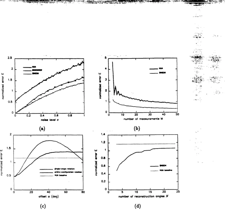
In Figure 5a, we show a plot of E versus measurement noise level Oa for each of the three algorithms, with M = 24 uniformly-spaced measurements of the standard triangle. While the error for all three algorithms increases with a as expected, the performance of BNGONROT is much better than that of NUA but only slightly worse than that of BNGON for relatively low noise levels. The difference in performance between BNGON and BNGONROT becomes more pronounced near a = 0.17. This threshold effect is exactly that characterizing standard nonlinear estimators, and is analyzed below and in more detail in [13]. However, even with this increased degradation, BNGONROT's performance is much better than that of NUA. Figure 5b shows a plot of E versus number of measurements M for NUA and BNGON, with noisy (a = 0.25) measurements of the standard triangle. Again, BNGON outperforms NUA, where both yield decreasing values of E with increasing M.

The performance of BNGON and BIGONIROT is also dependent on the quality of the prior infor-mation. For example, let us examine the sensitivity of BIGON. Specifically, we take M = 24 noisy

(oa = 0.25) measurements of the standard triangle. However, we reconstruct a triangle whose face

angles are not the same as those of the standard triangle. Errors in the reconstruction angles considered are entire-configuration errors in which all face angles are rotated by the same amount, and single-angle errors in which only the first reconstruction angle, originally at 7.125°, is in error. The angular error is denoted by a. Figure 5c depicts plots of error E versus a for the two types of errors in the prior. A dashed line denoting the baseline performance level of IUA is included for comparison. The figure indicates that for values of a less than 69°, entire-configuration errors are less damaging than corresponding single-angle errors. Moreover, on noting the intersections of the BNGON plots with the NUA baseline, we may conclude that for this particular noise level, one should tolerate single-angle errors of up to z 17° and entire-configuration errors of up to ; 290 before abandoning the BiGON algorithm and resorting to either BIGONROT or NUA.

Obviously, knowledge of the precise number of sides of the desired reconstruction is a very powerful and, in some sense, unrealistic piece of prior information. Thus, it is of interest to see how BNGON performance degrades as the number N of reconstruction angles is increased. To do this, we again use 24 uniformly-spaced noisy (a = 0.25) measurements of the standard triangle. We start with the correct triple of reconstruction angles at dl = 7.1250, q2 = 82.8750, and d3 = 2700 for

N = 3. For all values of N > 3, we choose ON such that it lies halfway between the most distant

adjacent pair of the previous N - 1 reconstruction angles. For each value of N, we solve the resulting BNGOIN problem in a Monte Carlo fashion in order to generate a data point in Figure 5d. Through this constructive process, a constellation of 24 more or less uniformly-spaced reconstruction angles is built up. The performance of BJGON for the set of reconstruction angles constructed in this manner is compared with the baseline performance of NUA, which uses the set of 24

uniformly-spaced measurement angles. From the plot, we may conclude that for a polygon of N sides, as long as the N reconstruction angles are known, adding extraneous reconstruction angles degrades performance but not to the extent that switching to NUA is better. This is particularly apparent from the fact that BNIGON performs significantly better than IUA near N = 24, indicating that the original three reconstruction angles that are not available to NUI are quite helpful to BIGON.

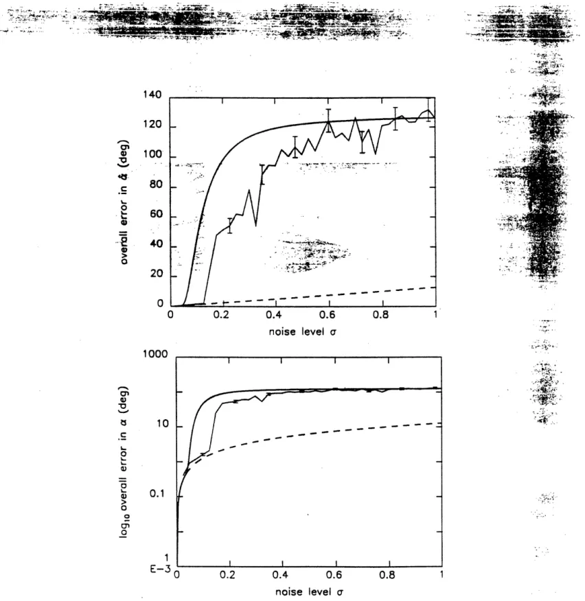
Finally, we investigate the performance of BNGONIROT in estimating the orientation parameter a. In Appendix C, we analytically determine the Cramer-Rao lower bound [16] on the orientation error variance as well as an approximate expression for the probability of obtaining anomalous orientation estimates (the 'threshold phenomenon' mentioned previously). Together, these expressions describe the orientation error variance for a range of noise levels, and is given by

var(a -

6latrue)

1

H1

--

2[

+ -exp ( 2) (180)2. (17)

where the probability Pr(A) of anomalous orientation estimate, the Cramer-Rao bound CRB, and

H are given in Appendix C.

Monte Carlo simulations supplementing this analytical error analysis were also performed. As before, we use M = 24 uniformly-spaced measurements of the standard triangle so that the true orientation, or offset parameter is given by atru = 90° . _{Figure 6 compares the analytical expression}

for the standard deviation of the orientation estimate with the Monte Carlo results, for a range of noise levels. Plots of /var(a - &l-atru) versus o are shown on both normal and logarithmic scales, with each Monte Carlo data point representing 200 noise realizations. The Monte Carlo results agree reasonably well with (17) and, as expected for a nonlinear estimator, exhibit dramatic

threshold behavior as the noise variance increases from low values, where the CRB dominates, to

higher values, where Pr(A) is significant.

4. LASER RADAR DATA AND EXTRACTION OF SUPPORT LINE MEASUREMENTS

In this section, we describe the laser radar data to be used as input to the reconstruction

algorithms (namely, range-resolved and Doppler-resolved data). We then discuss the way in which

the laser radar data can serve to provide support line information, and describe a technique to

extract such support measurements from the data. Previous work in reconstructing targets from

such laser radar data have primarily employed techniques from transmissive tomography [7, 17].

These transmissive tomographic techniques are designed to provide reconstructions of an object's

mass density given measurements of line integrals of this mass density. Although the application

of these techniques to laser radar data provide reconstructions containing some geometric qualities

of the target, it is not at all clear what the reconstructed intensities represent. Our motivation in

using convex set reconstruction techniques stems from the fact that although the laser radar data

do not convey line integral information, they do in fact provide target support information.

4.1 Laser radar data and problem scenario

By illuminating a target and receiving the reflected signal, laser radars provide information

about the surface characteristics of the target. Laser radars can be designed to resolve the return

from the target with respect to various quantities [18, 19]. In this paper, we restrict attention to

range-resolved and Doppler-resolved laser radar data. Furthermore, we consider only the case of a

monostatic radar, in which the transmitter and receiver are at the same location.

A range-resolved measurement (also called a range spectrum) is one in which the return is

distributed in range along the line of sight (LOS) of the laser radar. That is, only those parts

of the target that are a distance ro away from the laser radar (with distance measured along the

LOS) may contribute to the value of the range spectrum at range ro. Although a range-resolved measurement ideally has perfect range resolution, in practice it takes the form of a histogram with bins of finite range extent, where each bin is referred to as a range bin.

Alternatively, for a target undergoing motion, different parts of the target may have different components of velocity along the LOS. A Doppler-resolved measurement (also called a Doppler spectrum) is one in which the return is distributed with respect to these variations in velocity. As with a range spectrum, the Doppler spectrum takes the form of a histogram. The value associated with a particular Doppler bin arises from the return of all illuminated parts of the target with the corresponding component of velocity along the LOS.

The received intensity from a surface illuminated by a laser radar is dependent on the geometry and reflectance properties of the surface. The reflectance properties are commonly characterized by a function known as the bidirectional reflectance distribution function (BRDF) [20]. For the case of a monostatic radar and a surface with isotropic reflectance properties, the BRDF is given by p(t) where

4

0 = 2lr J p(,b)cos2 dA, (18) where the integration is performed over the visible (illuminated) part of the surface, denoted by S. The quantity a is referred to as the laser radar cross section (LRCS) of the target. Hence, for resolved data, the intensity value associated with a particular bin is proportional to the LRCS

arising from those portions of the target that contribute to that bin.

In this paper, we investigate some methods to reconstruct a target from a series of range-resolved or Doppler-range-resolved measurements using the algorithms described in the preceding section.

Throughout, we consider only the case in which the data is taken at aspects around a great circle, so that the lines of sight all lie in a plane. With this restriction, the entire scenario is reduced to a two-dimensional problem in the plane containing the lines of sight.

For range-resolved measurements, we can consider the data as being obtained either with a single sensor revolving around a stationary target, or with the sensor fixed and the target rotating, with known rotation rate, about an axis perpendicular to the plane in which the measurements are taken. For Doppler-resolved measurements, target motion is required to resolve the target, and so in this case we assume that the target is rotating as above with a fixed sensor.

Alternatively, in either case we may think of the data as being obtained simultaneously by a number of sensors distributed about the target. Also, as in previous work using tomographic techniques [7, 21, 17], we make several assumptions. Specifically, as we shall see, knowledge of the relative positions of the sensors is needed to reconstruct targets from both range-resolved and Doppler-resolved measurements. In addition, for Doppler-resolved measurements, we assume that the target is rotating about an axis perpendicular to the plane of aspects, with known rotation rate. Moreover, if the target is translating, the Doppler velocity of the target's center of gravity relative to each sensor must be known. Since each sensor is presumably tracking the target, we assume knowledge of the necessary quantities. In what follows, we view the problem from this multi-sensor

perspective.

4.2 Support line measurements from laser radar data

Given a range-resolved measurement, the minimum range rtin with nonzero return intensity indicates that the distance from the sensor to any part of the target is at least rmn. Under far-field assumptions, the above indicates that the target lies completely on one side of the plane perpendicular to the LOS at range rmin. Moreover, since some part of the target is at range

rsns, this plane actually grazes the target. Hence, this plane is precisely a support plane of the target. (Note that the maximum range rmax with nonzero return intensity does not necessarily provide another support line, since parts of the target at ranges greater than rmax may not be visible to the radar.) However, under our restriction that the LOS's all lie in plane, the problem is effectively reduced to a two-dimensional one, as mentioned above. That is, we need only consider the projection of the target in the plane of LOS's. The support plane information contained in the data corresponds to support line information of the target's projection. Hereafter, use of the word 'target' refers to the two-dimensional projection of the actual target.

A Doppler-resolved measurement contains similar information. For a target undergoing simple rotation with known rate w, the Doppler frequency due to a point on the target is proportional to the distance from the point to the rotation axis in a direction perpendicular to the LOS (also called the cross-range distance of the point). The minimum and maximum Doppler frequencies, Dmin and

Dmax, with nonzero return intensity correspond to the minimum and maximum cross-range of any

part of the target. Thus, from a Doppler-resolved measurement we can extract two lines parallel to the LOS that graze the target which lies between them. Hence, two support lines of the target are obtained in this case.

To identify the support value(s) associated with the support line(s) provided by a range or Doppler spectrum, a coordinate frame is needed. This frame must serve as a common reference for all of the aspects, so that the sets of data may be spatially aligned, or registered. For range-resolved measurements, the assumption that the positions of the laser radars are known relative to one another allows us to establish such a frame, say, with origin at the average of the laser radar position coordinates and 0° aspect defined by the LOS of the first laser radar. The resulting position and orientation of this coordinate frame is, of course, arbitrary. Given such a coordinate frame, the support value corresponding to the it h laser radar's range spectrum is equal to the minimum

nonzero range rmin subtracted from the distance from the laser radar to the origin along the ith LOS. The set of support values obtained in this manner for the set of laser radars forms a support vector y.

A coordinate frame for Doppler-resolved measurements is established in the same way as for

range-resolved measurements. From above, the ith sensor (at aspect Oi) gives rise to support values

at Oi + 900. Since target cross-range is proportional to Doppler frequency after shifting the Doppler spectrum by the Doppler frequency shift Di produced by the target's translational velocity relative

to the sensor, the support values are given by m - Dil and gDmax - Dil, where A is the

wavelength of the laser illumination.

Since a Doppler spectrum at aspect Oi provides two support values, at 8i + 90°, the aspects 8i

and Oi + 1800 yield duplicate support values, if the support values are free of noise. For noisy data, the duplicate values may be averaged, thereby reducing the noise in the support measurements.

In general, the resulting support vector y arising from range or Doppler data is noisy and may be invalid, due to two types of measurement errors. One type of error arises in incorrectly estimating the values of rmi, or Drain and Dmax amid noise in the range or Doppler spectra. The technique used to estimate rmin, Dmin, and Dmax from the laser radar data is briefly described in Section 4.3. Secondly, incorrect knowledge of the relative laser radar positions (and for Doppler data, incorrect knowledge of the Doppler velocity of the target's center of gravity relative to each sensor) leads to registration errors. Errors in knowing the laser radar positions may also cause angular errors (i.e., errors in knowing the aspects). However, in this paper we ignore angular errors and assume throughout that the aspects of the measurements are known perfectly.

4.3 Knot location

noisy data is a quite difficult problem in general. The most obvious method-thresholding the data-suffers greatly from its nonrobustness to noise 'spikes' in the data. As a result, we turn to a method based on a technique developed by Willsky and Jones [22] for detecting abrupt changes in dynamic systems, and later applied by Mier-Muth and Willsky [6] to spline estimation. To cast our problem in the framework of [6], we model the range or Doppler spectrum as a linear spline, or piecewise linear function. The points of discontinuity in derivative are referred to as knots. Our goal is to determine the first knot in a range spectrum and the first and last knots in a Doppler spectrum.

The basic approach consists of using a Kalman filter based on a linear ramp model for the range or Doppler spectrum. Initializing the filter with zero slope, we run the filter along the spectrum. At each bin, we use the innovations sequence to determine a set of maximum-likelihood (ML) estimates of the slope of the ramp at the current bin assuming that a knot was located at each of the previous bins in some finite window. Using the ML estimates for each bin in the window, we perform a generalized likelihood ratio (GLR) test for the two hypotheses 'knot present' and 'knot absent' in order to determine whether a knot actually exists at the locations of any of the ML estimates. The first bin for which the GLR exceeds a prespecified threshold corresponds to the first knot in the spectrum. For a Doppler spectrum, to locate the last knot, we repeat the above process running the Kalman filter backwards along the spectrum. Details concerning the implementation and performance of this algorithm may be found in [22], [6], and [5].

In concluding this section, we note that it is in general more difficult to locate knots in a Doppler spectrum than in a range spectrum. This difference is due to the properties of typical target materials combined with the viewing geometries associated with the two data types [21]. In particular, the values of the laser radar return at ranges just higher than rmin are determined by parts of the target whose surface normals roughly coincide with the LOS. As a result,

4

'

maximizing cos l in (18). Furthermore, since materials typically give high intensity return at

near-normal incidence and low intensity return at near-grazing incidence, the BRDF p(4') is near maximum. Hence, range spectra generally exhibit an abrupt increase in intensity at the knot having range rain- In contrast, the values of the laser radar return at Doppler velocities just greater than Dmin and just less than Dma, are determined by parts of the target having surface normals that

are nearly perpendicular to the LOS. Consequently, 0i/ ~ 90° giving rise to values of cos i/ and p(t/')

that are nearly zero. Hence Doppler spectra generally vary slowly in intensity near the two knots.

5. TARGET RECONSTRUCTIONS FROM LASER RADAR DATA

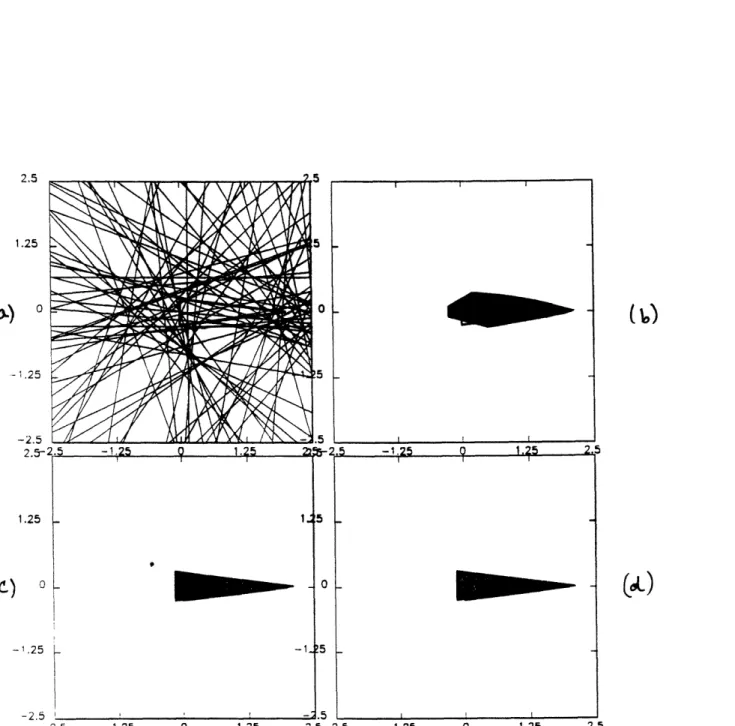
In this section, we apply the knot location technique discussed in Section 4.3 and the convex set estimation algorithms of Section 3 to laser radar measurements of several targets, in order to obtain shape estimates of the targets. The examples presented are those of reconstructions from sets of range and Doppler spectra obtained through simulated, laboratory, and field measurements. The data for the first two examples are simulated [23] range-resolved and Doppler-resolved mea-surements of a cone of height 200 cm and radius 25 cm with Lambertian reflectance characteristics. The cone is positioned with the center of its base at the origin of a coordinate frame and oriented such that its axis of symmetry lies in the xy-plane. In order to be resolved in Doppler, the cone rotates in the xy-plane about the z-axis at one revolution per second, in a manner resembling end-over-end tumble. Measurements are taken at an instant in time when the cone's axis is aligned with the frame's z-axis, at 72 aspects uniformly-spaced around the great circle of radius 10,000 in in the xy-plane, and with a resolution of 2 cm for the range data and a resolution of 3.750 KHz for

the Doppler data.

To reconstruct the targets, we first locate the knots by the Kalman filtering technique described in Section 4.3 and convert them to support values. Modelling knot location errors and registration

errors for each aspect by statistically-independent samples from zero mean Gaussian distributions with variances a2 _kI and a2 _reg, the effective measurement error is Gaussian, with variance a2 =

al + a2¢g for range-resolved data. However, for Doppler-resolved data at an even number of

uniformly-spaced aspects, (1) registration errors for aspects 1800 apart are negatives of each other, and (2) the duplicate support value measurements provided by aspects 1800 apart are averaged together. As a result, the knot location error may be modelled by drawing samples from a Gaussian distribution with variance ard/2 for each aspect. The registration error may be obtained by drawing samples from a Gaussian distribution with variance

a2eg/2

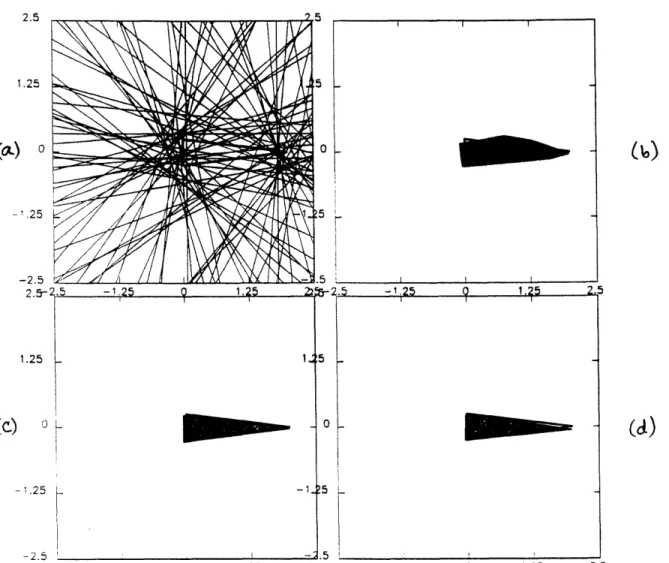
The support lines resulting from locating knots and corrupting the support values by measure-ment noise are shown in Figure 7a for range-resolved data, with noise level aeff = 0.50 m. The reconstructions produced by NUA, BIGON, and BIGONIROT from this set of noisy support line measure-ments are shown in Figures 7b-d. The display conventions of this figure will be used throughout this section. The reconstructions exhibit behavior similar to that seen for the standard triangle reconstructions of Sections 3.1-3.3. In particular, the prior knowledge of relative reconstruction angles allows BNGONROT to outperform NUA dramatically, but does not cause it to underperform BNGON significantly, which uses absolute angle information. Also, the quality of the reconstructions is rather impressive in light of the fact that the noise level is so high, having a standard deviation equal to the full width of the target. The corresponding results for the Doppler-resolved measure-ments arising from knot location error (orkl = 0.25 m) and registration error (Oreg = 0.25 m) are shown in Figure 8.

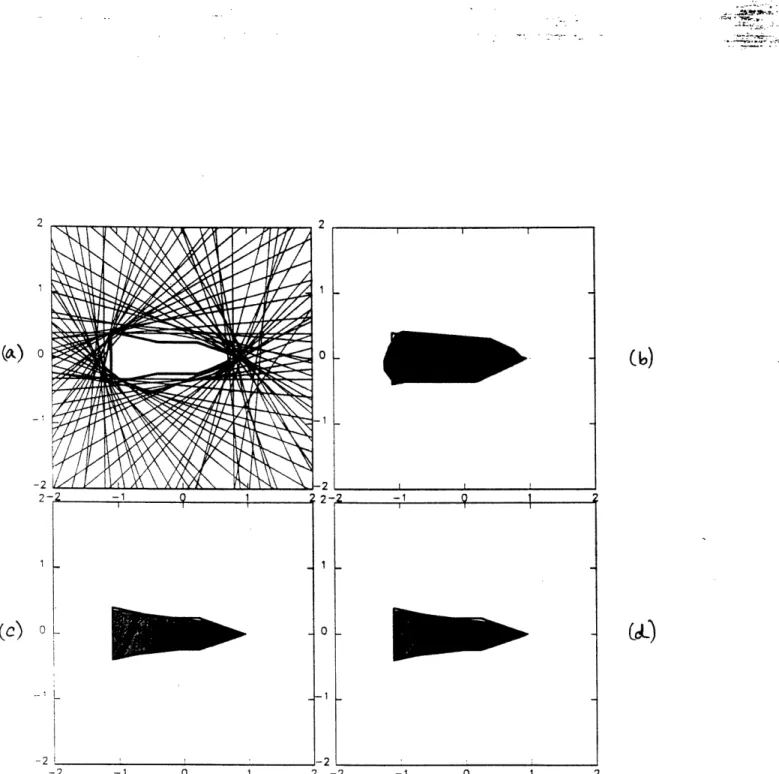
The next example is one of reconstructing a triconic target of height 203 cm and base radius 39.5 cm (shown outlined in Figure 9) given laboratory range-resolved measurements. The

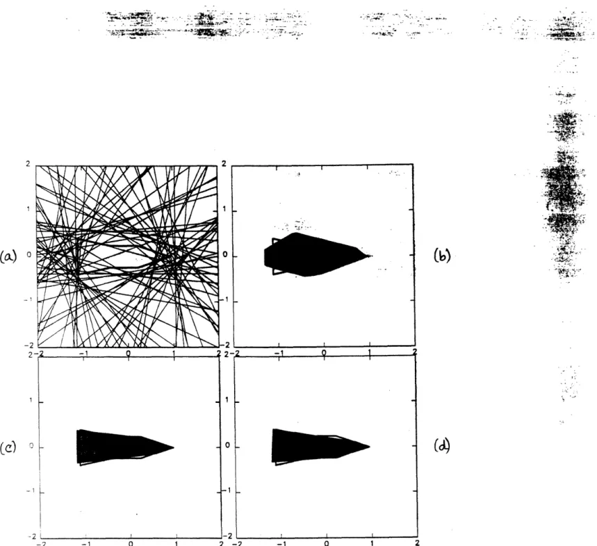
labora-tory measurements were taken on a ten meter indoor range at 72 uniformly-spaced aspects in the horizontal plane containing the target's axis of symmetry, with a range resolution of 1 cm. See [7] for details of the experimental set-up. Support lines and reconstructions using the three estimators are shown in Figure 9 for the uncorrupted laboratory data and in Figure 10 for the laboratory data corrupted with measurement noise (aoeff = 0.25 m). Note that since the target is not convex, support values using BINGON and BNGONROT are reconstructed at five angles corresponding to the sides of the convex hull of the target.

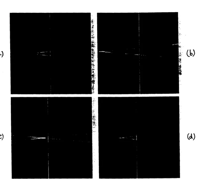
Finally, we present reconstructions from Doppler-resolved field measurements. The target, a scaled aluminum model of the Thor-Delta rocket body (shown outlined in Figure 11a), was rotated at approximately 1 rpm about an axis normal to its axis of symmetry. The measurements, taken at 72 aspects in a plane normal to the rotation axis, were made using a 10.6/Lm CO2narrowband laser radar on a 5.4 km ground range, and had a Doppler resolution of approximately 200 Hz. Details of the experiment may be found in [7]. Support lines and reconstructions produced by the three algorithms are shown in Figure 11 for the uncorrupted field data and in Figure 12 for the field data corrupted with measurement noise (o<d = 0.10 and ,reg = 0.10). Again, since the target is not convex, support values using BNGON and BNGONROT are reconstructed at eight angles corresponding to the sides of the convex hull of the target.

5.2 Comparison with and Improvements to Tomographic Imaging Methods

In previous work, standard methods of tomographic image reconstruction [241 were applied to range-resolved and Doppler-resolved laser radar data [7, 17]. In this section, we compare the convex set reconstructions of the previous section with reconstructions produced using the tomographic methods. We then examine the effect of registration errors on both methods. As we shall see, the present algorithms are quite robust to registration errors, in contrast to tomographic

recon-structions, which are rather sensitive to these errors. Finally, we show that the robustness of the present algorithms can be used to dramatically improve tomographic reconstructions from data with registration errors.

All of the tomographic reconstructions in this section were obtained using the standard method of filtered backprojection. (See [24] for methods of transmission tomography, and [7, 17] and references contained therein for the application of these methods to laser radar reflective data.) Parts (a) of Figures 13-16 show filtered backprojection reconstructions from the four data sets (free of registration errors) used in Section 5.1. It should be noted that the Doppler data sets were thresholded prior to being backprojected in order to improve the tomographic reconstructions. This is necessary since typically the high intensities are near the center of a Doppler spectrum and tend to give rise to a dominant high intensity region in the center of the reconstruction. Incidentally, we threshold the data sets prior to backprojecting rather than thresholding the reconstructed images themselves, since the former approach appears to yield better results.

Unlike the convex set reconstructions (shown in parts (b)-(d) of Figures 7-12), the tomographic reconstructions contain intensity information within the outline of the target. However, exactly what information the intensity values convey about the target's surface is not well understood. Furthermore, the tomographic images differ from their convex set counterparts in that they do not provide direct size or shape estimates of the target. While, in principle, techniques to extract edge and shape information could be used, the usual difficulties associated with image processing would be faced. This is especially true of reconstructions arising from Doppler data, where for reasons suggested in Section 4.3 and described and demonstrated in [21], reconstructed edges are not highlighted but are instead overwhelmed by the high intensities that are reconstructed in the interior of the target. Even when using thresholding as mentioned above, edges in the reconstructions from Doppler data are not sufficiently highlighted.

Like the convex set algorithms, tomographic techniques require knowledge of a common ref-erence point, without which registration errors occur. The introduction of registration errors in the data has disastrous effects on the tomographic reconstructions that result. Parts (b) of Fig-ures 13-16 show the tomographic reconstructions resulting from shifting the data in each spec-trum by an amount given by a zero-mean Gaussian random variable with standard deviation 0'reg = 0.50, 0.25, 0.25, and 0.10 m (with the shifts for the spectra being independent of one another,

except for the Doppler data sets, where shifts for aspects 1800 apart are negatives), and then using filtered backprojection. Clearly, one cannot expect any image processing algorithm to successfully extract shape information from the tomographic images in these figures.

In contrast, the convex set algorithms are rather robust to registration errors. This is seen from the reconstructions shown in parts (b)-(d) of Figures 7,8,10, and 12, obtained from data suffering from the identical registration errors as those used for the tomographic reconstructions (i.e., the same noise realizations were used), as well as knot location errors with the same standard deviations as above.

The difference in the robustness of tomographic and convex set methods to registration errors is due to the fact that the convex set algorithms attempt to register the data in the reconstruction process using implicit information as to the consistency of the measurements. That is, in adjusting the support values to achieve consistency, the algorithms are essentially shifting each range or Doppler spectrum such that the sum of the squares of the shifts is minimal and such that the set

of shifted laser radar data is registered data for some target.

In fact, we may exploit this registering property of the convex set algorithms as an aid to tomography, for data sets with registration errors. Specifically, we start with a possibly inconsistent set of measured support values {yi}, which are estimated from the laser radar data by knot location. If we have no prior information as to the target's shape, we use NUA to obtain a consistent set of

support values {hi}. If we have prior shape information, we use BIGON or BNGONROT to estimate a consistent set of support values at the reconstruction angles, and then sample the (piecewise-sinusoidal support function of the reconstructed polygon at the measurement angles to yield a consistent set of support values {hi). Then, given the {hi) and {yi), we shift the ith range or Doppler spectrum by an amount hi - yi, for all values of i. The resulting registered data set is then processed tomographically by filtered backprojection.

Parts (c) and (d) of Figures 13 and 14, parts (c)-(e) of Figure 15, and part (c) of Figure 16 show the tomographic reconstructions that result using this process. The tomographic reconstructions resulting from preprocessing by each of the three convex set algorithms are not included in some of

the figures. In the cases that the reconstruction corresponding to BNGON was omitted, it could not be distinguished from that corresponding to BNGONROT. In the case where reconstructions for both

BNGON and BIGONROT were omitted, they were indistinguishable from that corresponding to NUA.

Quite clearly, on comparing the various images within each of the Figures 13-16, the improvement obtained using the registration correction method is dramatic.

6. SUMMARY AND SUGGESTIONS FOR FURTHER WORK

In this paper, we first developed and studied several techniques for estimating convex sets from a set of noisy support line measurements. The basic approach to these methods involves reconstruct-ing a polygon close to the measurements while enforcreconstruct-ing a consistency condition and utilizreconstruct-ing prior information, if available. The algorithms are computationally feasible with two of the estimators resulting in quadratic programming problems and the third having a quadratic programming core. The performance of the algorithms was assessed with respect to several parameters. As expected, if accurate prior information is available then BNGON and BIGONROT substantially outperform JUA. A useful observation is that the performance of BIGONROT is comparable to that of BNGON while

elim-inating the need for prior orientation information. The ability of BNGONROT to provide orientation estimates may be useful in certain applications.

We also introduced the use of these methods for reconstructing targets from resolved laser radar data. The reconstruction process consists of first extracting support line measurements from the data, and then producing a shape estimate using the convex set estimation techniques. The application of these techniques to laser radar data obtained through simulated, laboratory, and field measurements was demonstrated. The reconstructions obtained were compared to those produced by tomographic imaging methods, resulting in the following observations. First, shape estimates are explicitly provided by our algorithms, as opposed to tomographic images, which can provide target shape information only after using image processing techniques with their attendant difficulties. Second, we investigated the effects of registration error on both methods and found that the tomographic methods experience substantial degradation, unlike the present methods which are rather robust. These observations motivated us to exploit the tendency of our algorithms to correct unregistered data, in an effort to improve the quality of tomographic images.

A variety of extensions to our reconstruction algorithms might be made. One such extension may consist of developing more general formulations of the best N-gon algorithm, so that the use of less stringent prior shape information could be made. For example, one might consider a formulation in which only the number but not the values of the reconstruction angles are specified. A more general formulation might leave both the number and the values of the reconstruction angles unspecified, but would penalize larger numbers of reconstruction angles. Also, it may be interesting to develop algorithms that provide smooth shape estimates of objects, as opposed to polygonal estimates. Incorporating the effects of noise in the measurement angles may be useful in some applications. Another useful generalization would be to extend the algorithms to three