A continuous approach to information-theoretic exploration with range sensors

A Continuous Approach to Information-Theoretic

Exploration with Range Sensors

by

Trevor Henderson

Submitted to the Department of Electrical Engineering and Computer

Science

in partial fulfillment of the requirements for the degree of

Master of Engineering in Computer Science

at the

MASSACHUSETTS INSTITUTE OF TECHNOLOGY

September 2019

© Massachusetts Institute of Technology 2019. All rights reserved.

Author . . . .

Department of Electrical Engineering and Computer Science

August 23, 2019

Certified by. . . .

Sertac Karaman

Associate Professor of Aeronautics and Astronautics

Thesis Supervisor

Certified by. . . .

Vivienne Sze

Associate Professor of Electrical Engineering and Computer Science

Thesis Supervisor

Accepted by . . . .

Katrina LaCurts

Chair, Master of Engineering Thesis Comittee

A Continuous Approach to Information-Theoretic Exploration

with Range Sensors

by

Trevor Henderson

Submitted to the Department of Electrical Engineering and Computer Science on August 23, 2019, in partial fulfillment of the

requirements for the degree of

Master of Engineering in Computer Science

Abstract

In this thesis we derive an algorithm that addresses the computational bottleneck of robotic exploration: computing the expected information gain — i.e. mutual informa-tion — between an occupancy map and a range sensor measurement. The algorithm we derive has a lower complexity and in practice runs 200 to 1500 times faster than the state of the art CSQMI and FSMI algorithms. The speedup is due to the real-ization that the mutual information at one cell of an occupancy map can be defined in terms of the mutual information at adjacent cells. This makes computing the mutual information at all cells in the map much faster than computing the mutual information of each cell independently.

The derivation is unique in that it models the occupancy map and range measure-ments as continuous random fields despite the fact that actual computation requires quantization. This framework is critical to the recursive definitions that provide per-formance gain. It also reveals flaws, previously obscured by discretization, in several well established concepts: the practice of initializing occupancy probabilities in an occupancy grid to 1/2 is arbitrary and in application often an overestimate; and the formula for mutual information defined by Julian et al. fails to take into account a radial volume element, which changes mutual information values dramatically. Both of these claims are supported empirically.

Finally, we investigate two heuristics that use mutual information computation to perform actual exploration tasks and provide an analysis of each heuristic’s use case. These claims are validated by synthetic exploration experiments.

Thesis Supervisor: Sertac Karaman

Title: Associate Professor of Aeronautics and Astronautics Thesis Supervisor: Vivienne Sze

Acknowledgments

My deepest gratitude to the people who made this thesis possible:

To my advisors Sertac Karaman and Vivienne Sze for their support, patience and wisdom; for giving me the freedom to let my research wander; for long nights spent together cramming for papers and demonstrations; and for their understanding when things go awry.

To Zhengdong Zhang for introducing me to the problem studied in this thesis, for his own foundational work and for his unending positivity.

To my labmates past and present for their feedback and camaraderie; to Soumya Sudhakar, Peter Li, Diana Wofk, Tien-Ju Yang, Fangchang Ma, and Amr Suleiman. To Luca Carlone for supporting me as a TA and to reset of the 6.141 staff, espe-cially to Corey Walsh for his mentorship.

To my Beaverworks colleagues; to Andrew Fishberg for making me smile, driving me home, and all of our Racecar adventures.

To my friends on Long Island for all the times they’ve welcomed me home and made it feel like I never left. To my roommates and neighbors for family dinners, movie nights, Sunday Magic, pool at The Field and making music. To Senior House and the ongoing Death House after-party. And to my radio co-host Ru and our month-long writing marathon without which this thesis would not exist.

To my grandparents for their generous support and life advice over the years. And, with love, to my parents — who I will certainly call back after I turn this in — who once told me they would take me to Legoland if I could work out how to make a Lego sphere and followed up on their promise; and most of all to my brother Dylan.

Contents

1 Introduction 11

1.1 Related Work . . . 13

1.1.1 Mapping . . . 13

1.1.2 Next Best View Exploration . . . 14

1.1.3 Next Best Path Exploration . . . 16

1.2 Thesis Contributions . . . 17

2 Definitions and Notation 19 2.1 Occupancy Maps . . . 19

2.2 Range Measurements . . . 21

2.3 Information Theory . . . 21

2.4 Information Theoretic Exploration . . . 21

3 Choosing the Next Best View: Computing Mutual Information 23 3.1 A Formula for the Mutual Information𝐼(𝑀 ; 𝑍x,Θ) . . . 24

3.2 Density Functions of Range Measurements . . . 26

3.3 A Piecewise Vacancy Assumption . . . 27

3.4 Algorithm 1: For Barely Distorted Range Measurements . . . 32

3.5 Algorithm 2: For Symmetrically Distorted Range Measurements . . . 37

4 Choosing the Next Best Path: Ask a Salesman 45 4.1 Justifying Nearest Neighbor Exploration . . . 47

4.3 A Conditional Heuristic . . . 49

4.4 Computing Conditional Mutual Information . . . 50

4.4.1 An Upper Bound . . . 54

4.4.2 A Lower Bound . . . 54

5 Experimental Evaluation 57 5.1 The Speed of Algorithm 1 . . . 58

5.2 The Accuracy of Algorithm 1 . . . 59

5.3 Empirical Justification of the Volume Element . . . 60

5.4 Empirical Verification of the Conditional Bounds . . . 62

5.5 The Effect of the Unknown Prior on Mutual Information . . . 62

5.6 The Effect of Distortion . . . 67

5.7 A Comparison of Next Best Path Heuristics . . . 69

6 Conclusion 75 6.1 Future Work . . . 76

6.1.1 Applications . . . 76

6.1.2 Complexity . . . 76

6.1.3 Guarantees and Bounds . . . 77

List of Figures

3-1 A Visualization of the Notation Presented in Lemma 3.1 . . . 28

3-2 A Visualization of the Results of Lemma 3.1 . . . 29

3-3 An Aid to Understanding Lemma 3.6 . . . 40

4-1 The Next Best Path Problem is NP-hard . . . 46

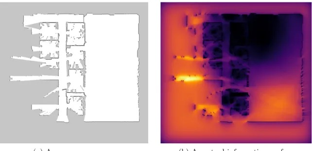
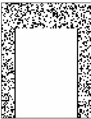
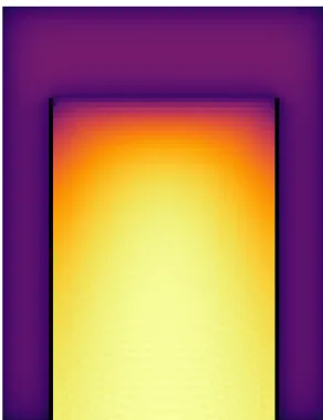
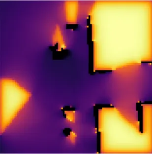
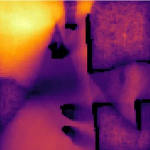
5-1 Mutual Information in an Incomplete Map of MIT’s Building 31 . . . 58

5-2 Monte Carlo Mutual Information Computation . . . 63

5-3 Mutual Information Surfaces Corresponding to Figure 5-2a . . . 64

5-4 The Effect of the Volume Element in a Real Environment . . . 65

5-5 Bounds on the Conditional Mutual Information . . . 66

5-6 The Effect of the Unknown Prior on Mutual Information Surfaces . . 68

5-7 The Map’s Entropy during Evaluation of Different Exploration Heuristics 72 5-8 The Paths Traversed by Different Exploration Heuristics . . . 73

Chapter 1

Introduction

Exploration is the task of charting an informative map of an environment under a set of resource constraints; time, energy, travel distance, etc. This is a critical component of robotic systems that are designed to navigate autonomously in unknown environments with application to space exploration, crop survey and disaster response. In this thesis we work towards an efficient exploration strategy for a range-sensing robot that equates charting an informative map to charting a map with minimal entropy.

Most notably, we derive a state of the art algorithm that computes how the map’s entropy 𝐻 is expected to change if a range measurement is made from point x with field of view Θ. Equivalently, this algorithm compute the mutual information 𝐼 between the map 𝑀 and the range measurement 𝑍x,Θ.

𝐼(𝑀 ; 𝑍x,Θ) = 𝐻(𝑀 )− 𝐻(𝑀|𝑍x,Θ) (1.1)

Computing expected information gain is necessary for most modern exploration techniques [10, 26, 44, 22, 12, 11, 5, 35, 23, 31, 6, 2, 9, 3]. For example, choosing the state (x, Θ)* _{that maximizes𝐼(𝑀 ; 𝑍}

x,Θ) is the next best view [12]; the measurement

state with the most potential to increase the information content of the map. Yet, the expected information gain, principally defined, is notoriously difficult to compute [26, 44, 10].

Considering a map divided into _{|𝑀| cells, algorithm 1 computes 𝐼(𝑀; 𝑍}x,Θ) at

every cell center x. The algorithm runs in time 𝑂(_{|Θ||𝑀|) where |Θ| is the number} of measurement beams within the field of view. This is a significant improvement over the state of the art CSQMI [10] and FSMI [44] algorithms which each take 𝑂(𝑙_{|Θ||𝑀|) to compute a similar quantity, where 𝑙 is the maximum range of the} sensor. This equates to a 200_{× to 1500× speedup in our experiments.}

The key to this performance gain is realizing that the mutual information at one cell can be defined in terms of the mutual information at an adjacent cell. This makes computing the mutual information at all cells in the map faster than computing the mutual information of each cell independently.

A unique aspect of our derivation is that it considers both the map and the range measurements to be defined continuously despite the fact that algorithm 1 eventually relies on quantization into cells and beams. This interpretation reveals a “bug” that exists in previous mutual information algorithms [26, 10, 44]: forgetting to account for the volume element in a radial integration. This bug makes a radical difference to mutual information values in 2D and 3D. The volume element is supported empirically by experiments that compute mutual information in a Monte Carlo fashion.

It also shows that the common practice of initializing occupancy values to 1/2 is misguided and can make mutual information computation a poor indicator of the actual expected information gain. This too is supported empirically.

We then turn to the more general problem of exploration problem that we call the next best path problem. The problem seeks a dynamically feasible path, with measurements made at every state along the path, that has the most potential to increase the information content of the map.

This problem is NP-hard but it is closely related to the traveling salesman problem which can be approximated in polynomial time [4]. Under this analogy, we investi-gate two heuristics for the next best path problem; one old and one new. The former, originally presented by González-Baños and Latombe, is at first glance ad hoc engi-neering but we provide insight into why it performs well and the conditions necessary for it doing so.

The latter is our own proposal, intended to work well when the González-Baños and Latombe heuristic does not. This heuristic relies on computing the conditional mutual information 𝐼(𝑀 ; 𝑍x,Θ|𝑍x0,Θ0. . . 𝑍x𝑘,Θ𝑘). While we do not provide an exact

algorithm, we provide constant time modifications to algorithm 1 that make it possible to compute upper and lower bounds of the conditional mutual information.

Chapter 2 begins by establishing the definitions and notations we use throughout the paper. Chapter 3 then derives efficient algorithms for computing 𝐼(𝑀 ; 𝑍x,Θ).

Chapter 4 shows how these algorithms can be used in two heuristics for the next best path problem. Chapter 5 details a number of experiments that verify the correctness of our algorithms, compare them to related methods and study the effect of different algorithm parameters. Chapter 6 concludes.

1.1

Related Work

1.1.1

Mapping

The problem of exploration is dependent on the ability to create a map. This work, like most others in the field, considers a system where the map is inferred through a series of range measurements. These measurements can be produced by many sensors including radar, sonar, lidar and stereo cameras. Recent advances in machine learning make it possible to accurately predict depth with a monocular camera [20, 21].

A common map representation for this sensor input is an occupancy grid [29]. The map is divided into equally sized regions and each is assigned an occupancy probability, i.e. the probability that the region contains an obstacle. Occupancy grids extend easily to 3D and data structures like Octomaps serve to make them more efficient by compressing regions with uniform occupancy probabilities [24]. To make updates to the occupancy grid tractable, the occupancy probabilities are assumed to be independent [29].

Occupancy grids are the primary choice for many exploration algorithms because they associate every region in the map with an occupancy probability. The downside

of these data structures is that they are quite large, especially in 3D [24, 40]. Many modern simultaneous localization and mapping (SLAM) algorithms for example use sparse maps like point clouds [32], meshes [16] and surfels [42]. While these maps are not probabilistic, is possible with mesh maps at least to associate every region with a state [35] — either occupied, vacant or unknown — each of which can be assigned a constant occupancy probability.

This work does not depend on the implementation details of the map so long as all regions of the map have an associated occupancy probability and the occupancy probabilities of non-overlapping regions are statistically independent. Some notable exceptions to the independence assumption are Gaussian process occupancy maps [34] and Hibert maps [36].

1.1.2

Next Best View Exploration

The earliest work on range-sensing exploration can perhaps be attributed to the art gallery problem posed in 1973 [33]. The problem asks how a minimal number of guards should be placed in an art gallery such that every point in the gallery is seen by at least one guard. One could view the solution as a minimal set of measurements a robot would need to make to produce a complete map of the gallery. The art gallery problem is, unsurprisingly, NP-hard [28].

The first practical exploration algorithm appeared in 1985 in the context of 3D modeling [12]. Rather than finding a globally optimal solution like the art gallery problem, Connolly [12] uses a local greedy strategy that at each step makes a mea-surement at the next best view, i.e. the sensor position that is expected to reveal the most information about the map.

One quality that discriminates various next best view algorithms is the metric used to quantify expected information gain. Many works, including the original, consider the information gain to be equal to the solid angle of unknown space visible from the sensor [12, 35]. Using terminology introduced in [43], this is measuring the visible area of the frontier. Other work considers information gain to be equal to the volume of unknown space that is visible to the sensor [11, 5, 22]. Both of these quantities are

computed via ray tracing.

In 2002, Bourgault et al. [6] introduced a more principled way to quantify informa-tion gain based on mutual informainforma-tion as described in equainforma-tion (1.1). In the earliest work, the mutual information was computed in a Monte Carlo fashion by averaging the resulting map entropy over random simulated range measurements [6, 2].

In 2015, Julian et al. [26] developed a non-stochastic expression for the mutual information that involves casting rays corresponding to each beam of the range mea-surement and performing a numerical integration over the cells that each beam in-tersects. The provided algorithm to compute the mutual information contribution between the map and a single measurement beam takes time 𝑂(𝑙2_𝜆

𝑧) where 𝑙 is the

maximum length of the beam and 𝜆𝑧 is an integration resolution.

By removing the numerical integration, Charrow et al. [10] produced the CSQMI algorithm which computes the mutual information between a map and a single mea-surement beam in 𝑂(𝑙2_{) and with a negligible approximation, 𝑂(𝑙). Rather than}

computing mutual information defined in terms of self-information they used an al-ternative information metric based on the Cauchy-Schwartz inequality [18]. While their metric is perceptually similar, the self-information cost function is the only local, proper and smooth cost function for an alphabet of size at least three [17, 30]. Using techniques similar to [10], Zhang et al. [44] produced the FSMI algorithm which also has an exact 𝑂(𝑙2_{) form and an approximate 𝑂(𝑙) form. The benefit of}

the algorithm is that it computes mutual information as traditionally defined rather than with a Cauchy-Schwartz cost function. It is also 2 to 3× faster than CSQMI due to its simpler form.

For context, algorithm 1 presented in this thesis computes the mutual information between the map and a single measurement beam in 𝑂(1) on average if the mutual information is computed at every cell in the map.

A separate timeline of exploration algorithms also exist that consider localization uncertainty, which is particularly useful for SLAM applications [7, 8]. Unfortunately, that history is outside the scope of this thesis, although it would be exciting for future work to consider whether the techniques presented here are applicable to such

systems.

1.1.3

Next Best Path Exploration

Any approach that seeks to maximize the information gain of each measurement will greedily minimize the total number of measurements. On modern systems however, recording and processing measurements takes a very small amount of time and energy relative to the actuation that moves the robot from place to place. We refer to the more general problem of determining a cost constrained path that maximizes expected information gain as the next best path problem.

An early next best path heuristic called frontier exploration declares a robot should move to the nearest frontier [43] where the frontier is again the boundary between free and unknown space. This heuristic is easy to describe and compute and in some cases still one of the best performing options [23].

Many of the next best view approaches listed above and otherwise augment their cost functions to prefer shorter paths. González-Banños and Latombe [22] choose the state that maximizes product of information gain and 𝑒−𝜆𝑑 where 𝑑 is the travel distance to the state. This method has subsequently been used in other work. [2, 5, 23]. Other approaches use ad hoc linear combinations of information gain, distance functions and other objectives like overlap [23, 3].

The authors of the CSQMI [10] and FSMI [44] algorithms generate shortest paths, compute mutual information along these paths and then follow the path with maxi-mal mutual information. Due to dependence between range measurements made at different points along a path, the joint mutual information between a map and all points on the path is much less than the sum of individual mutual information mea-sures. To account for this, Charrow et al. [10] introduce a method to lower bound the joint mutual information based on thresholding.

The shortest path heuristic is very computationally expensive since computing the mutual information at a single cell takes time 𝑂(𝑙|Θ|) and this must be done at every point of every path. Charrow et al. [10] and Zhang et al. [44] report downsampling the number of candidate paths, range measurement beams and measurement locations

to make this tractable. In practice this method performs only slightly better than frontier exploration [10, 44].

1.2

Thesis Contributions

1. A continuous framework describing occupancy maps and range measurements that is the basis of all of the results in this thesis.

2. An algorithm that computes the mutual information between an occupancy map and range measurements made at all cells in that occupancy map with a lower complexity and200 to 1500 times faster than the state of the art CSQMI [10] and FSMI [44] algorithms. This improvement owes to the insight that the mutual information in one cell can be defined in terms of the mutual information of its neighbors making joint computation cheaper than independent computation. 3. Several insights that violate the status quo: the occupancy probability of

un-known space is a context dependent parameter that shouldn’t be arbitrarily set to1/2; the mutual information between a map and a radial range measurement is not the sum of the mutual information between the map and 1-dimensional measurements.

4. A comparative analysis of heuristics that use mutual information to solve the more general next best path problem including a novel heuristic that uses con-ditional mutual information.

5. Empirical evidence that verifies the theoretical claims made in this paper, in-cluding a comparison of our algorithms to brute force numerical integration, a comparison between mutual information and stochastically-computed expected information gain, and synthetic exploration experiments.

6. A host of figures and qualitative analogies that explain how to interpret the results of our algorithms and their parameters in the hope that they are not treated as a black box.

Chapter 2

Definitions and Notation

2.1

Occupancy Maps

The following is a continuous generalization of occupancy grids [29] and other dense occupancy structures [35]. Aesthetically, this continuity makes deriving algorithms in chapter 3 cleaner without having to keep track of cell indices. But more importantly it makes it possible to evaluate a number of integrals analytically and brings to light of several key observations that are obscured by a discrete world.

For actual computation regular occupancy grids [29] can be used.

Definition 2.1. Given a probability space (Ω,ℱ, 𝑃 ), an occupancy map 𝑀 is a binary-valued random field indexed by points x _{∈ R}𝑛_{. The outcome of each binary}

random variable 𝑀x is either “free” or “occupied”.

Definition 2.2. Each point x_{∈ R}𝑛_{in occupancy map𝑀 has an occupancy 𝑜}

𝑀(x)∈

[0, 1] and a vacancy 𝑣𝑀(x) = 1− 𝑜𝑀(x). For any piecewise smooth curve 𝒞 ⊂ R𝑛

the probability that 𝑀𝒞 is free is equal to the continuous product of vacancies along

𝒞. 𝑃 (𝑀𝒞 is free) = ∏︁ x∈𝒞 𝑣𝑀(x)𝑑𝑠 (2.1) = exp (︂∫︁ 𝒞 log 𝑣𝑀(x) 𝑑𝑠 )︂ (2.2)

Remark 2.1. In occupancy grid mapping, works [26, 10, 44] intuitively consider the probability that a light beam passes through cells with occupancy probabilities 𝑜1. . . 𝑜𝑛 to be

𝑛

∏︁

𝑖=1

(1− 𝑜𝑖) (2.3)

Definition 2.2 directly generalizes this property to continuous space.

In this generalization however, one cannot equate the occupancy 𝑜𝑀(x) to the

probability that𝑀x is occupied. To shed some insight on the relation between

occu-pancy as we’ve defined it and occuoccu-pancy probability, consider a space with constant vacancy 𝑣. By definition 2.2,

𝑃 (𝑀𝒞 is free) = 𝑣 ∫︀

𝒞𝑑𝑠 _(2.4)

∫︀

𝒞𝑑𝑠 is simply the arc length of𝒞. If 𝒞 has unit length then the probability that 𝑀𝒞

is free is exactly equal to the vacancy. As _{𝒞 shrinks, the probability that 𝑀}𝒞 is free

grows exponentially and vice versa.

A particularly useful consequence is that occupancy and vacancy, unlike a dimen-sionless occupancy probability, are invariant to the map resolution. Dividing a region in two decreases the probability that the region is occupied, but does not effect its occupancy.

Remark 2.2. Many authors initialize their occupancy probabilities to𝑜𝑖 = 1/2 which

they claim is a state of zero information [29, 26, 10, 44, 36, 24, 34]. Using either the equation in definition 2.2 or the discrete equivalent mentioned in remark 2.1 one finds that this assumption is synonymous to the assumption that a beam of light travels through _{≈ 2 units in expectation.}

Two units is highly specific quantity and in our experiments almost always a gross underestimate of the distance a beam of light actually travels through unknown space. We explore how initial occupancy values effect information gain and consequentially robot behavior in §5.5.

2.2

Range Measurements

Similarly, the following definition generalizes the returns of many sensors including sonar, radar, and lidar.

Definition 2.3. 𝑅 is a random field consisting of range measurements 𝑅x,Θ. Each

𝑅x,Θ evaluates to a set of distances that measure from source point x ∈ R𝑛 to the

nearest occupied points of𝑀 within field of view Θ_{⊂ R}𝑛−1_{. Each angular coordinate}

𝜃 = (𝜃1. . . 𝜃𝑛−1)∈ Θ is a beam.

In this thesis we make a symbolic distinction between ground truth range measure-ments𝑅x,Θand distorted range measurements𝑍x,Θ. Two noise models are considered

in this thesis in sections 3.4 and 3.5 respectively.

Remark 2.3. Range measurements defined in definition 2.3 have no maximum range which is unrealistic for physical sensors and differs from previous exploration work [26, 44, 10, 5, 22]. Whether it is possible to achieve similar results without this assumption is left to future work. If the environment is more cluttered than the maximum range then the choice is irrelevant.

2.3

Information Theory

We make use of the information theoretic concepts mutual information, differential entropy and self-information. A thorough review of these concepts and the notation we use is found in [15].

Oftentimes we refer to the “mutual information of a state” which is an abuse of language intended to mean the “mutual information between a map and a range measurement made at a state.”

2.4

Information Theoretic Exploration

Finally, we reiterate the two important exploration problems: the next best view problem [12] and what we refer to as the next best path problem. The first approach

greedily minimizes the total the number of measurements to be made by choosing the information maximizing view at each step. The second approach also takes into account the cost of moving between states which makes it more applicable but also much harder to solve.

Definition 2.4. The next best view state (x, Θ)*

of a range sensor is the state that maximizes information gain of 𝑀 from observation 𝑍x,Θ in expectation.

(x, Θ)* = arg max

x,Θ

𝐼(𝑀 ; 𝑍x,Θ) (2.5)

Definition 2.5. The next best path 𝑄* _{is the path (a set of states (x, Θ) that can}

be connected dynamically), that maximizes information gain of 𝑀 from observation 𝑍𝑄 in expectation, subject to constraint 𝐷 on path cost 𝑑(𝑄).

𝑄* = arg max

𝑄

𝐼(𝑀 ; 𝑍𝑄) (2.6)

Chapter 3

Choosing the Next Best View:

Computing Mutual Information

This chapter derives efficient algorithms that compute the mutual information𝐼(𝑀 ; 𝑍x,Θ)

between a map𝑀 and distorted range measurement 𝑍x,Θ. These algorithms are

moti-vated by the fact that mutual information is necessary to solve the next best view [12] and next best path problems posed in definitions 2.4 and 2.5 which encapsulate the goals of autonomous exploration. Both algorithms have a lower complexity than the state of the art CSQMI [10] and FSMI [44] algorithms.

We establish a general formula for 𝐼(𝑀 ; 𝑍x,Θ) in §3.1. §3.2 completes the formula

by deriving an expression for the probability density function of a range measurement. With the goal of making the formula computationally tractable, §3.3 introduces a piecewise assumption about the map that makes it possible to evaluate many relevant expressions in closed-form. One particularly useful result shows that components of 𝐼(𝑀 ; 𝑍x,Θ) can be recursively defined in terms of components of 𝐼(𝑀 ; 𝑍y,Θ) for points

y adjacent to x. This result is key to producing algorithms with a lower complexity than CSQMI [10] and FSMI [44].

§3.4 and §3.5 use the results from §3.3 to produce two algorithms that compute 𝐼(𝑀 ; 𝑍x,Θ). The first computes the mutual information when the distortion in range

measurements 𝑍x,Θ is practically zero. The second computes mutual information

The distortionless algorithm is more practical and the one used in the rest of this thesis with the exception of a small discussion in §5.6.

3.1

A Formula for the Mutual Information

𝐼(𝑀 ; 𝑍

)

Theorem 3.1. Suppose measurements 𝑍x,Θ are range measurements 𝑅x,Θ with

dis-tances distorted by additive, independent, identically distributed noise𝑁 . The mutual information between map 𝑀 and 𝑍x,Θ is the sum of the mutual information between

𝑀 and individual measurement distances 𝑍x,𝜃 for beams 𝜃 ∈ Θ.

𝐼(𝑀 ; 𝑍x,Θ) =

∫︁

𝜃∈Θ

𝐼(𝑀 ; 𝑍x,𝜃) (3.1)

Additionally, 𝐼(𝑀 ; 𝑍x,𝜃) is equal to the difference of differential entropies,

𝐼(𝑀 ; 𝑍x,𝜃) = ℎ(𝑍x,𝜃)− ℎ(𝑍x,𝜃|𝑀) (3.2)

which can be defined in terms of probability density functions 𝑓𝑍x,𝜃(𝑟) and 𝑓𝑅x,𝜃(𝑟) of

the distorted and ground truth distances.

ℎ(𝑍x,𝜃) = − ∫︁ 𝑟∈R 𝑓𝑍x,𝜃(𝑟) log 𝑓𝑍x,𝜃(𝑟) 𝑑𝑉 (3.3) ℎ(𝑍x,𝜃|𝑀) = − ∫︁ 𝜌∈R 𝑓𝑅x,𝜃(𝜌) ∫︁ 𝑟∈R 𝑓𝑁(𝑟− 𝜌) log 𝑓𝑁(𝑟− 𝜌) 𝑑𝑉 𝑑𝜌 (3.4)

Proof. According to definition 2.2, the probability that any two disjoint curves are free is equal to the product of probabilities that each is free. This implies that range measurement distances𝑅x,𝜃 are independent across beams𝜃∈ Θ. Additionally, since

the noise𝑁 is independent, the distorted range measurement distances 𝑍q,𝜃 must also

be independent across beams𝜃 _{∈ Θ.}

Because of this independence, equation (3.1) follows directly from the definition of mutual information [15]. Equations (3.2) and (3.3) then follow from the definition of differential entropy [15]. Note that the volume element is 𝑑𝑉 = 𝑟𝑛−1_{𝑑𝑟𝑑𝜃.}

Other than it’s relation to 𝑅x,𝜃,𝑍x,𝜃 is independent of 𝑀 , so we can write

ℎ(𝑍x,𝜃|𝑀) = ℎ(𝑍x,𝜃|𝑅x,𝜃) (3.5)

For a fixed, known range measurement distance 𝜌, the differential entropy of 𝑍x,𝜃 is

equal to the entropy of the noise distribution translated by 𝜌.

ℎ(𝑍x,𝜃|𝑅x,𝜃 = 𝜌) = ℎ(𝑁 + 𝜌) (3.6)

Like equation (3.3), the differential entropy of 𝑁 + 𝜌 is

ℎ(𝑁 + 𝜌) =₋ ∫︁

𝑟∈R

𝑓𝑁(𝑟− 𝜌) log 𝑓𝑁(𝑟− 𝜌) 𝑑𝑉 (3.7)

Performing the expected value ofℎ(𝑁 + 𝜌) over 𝜌_{∼ 𝑅}x,𝜃 provides equation (3.4).

Remark 3.1. Other than being defined in a continuous setting, theorem 3.1 differs from the mutual information presented by Julian et al. [26] in two ways.

First of all Julian et al. assumes an explicit form of the inverse sensor model from [41]. However, the assumption overconstrains the problem; the inverse sensor model is already well defined via definitions of occupancy, range measurements and noise.

Secondly, Julian et al. does not account for the volume element. They assume that the mutual information between the map and a radial range measurement is equal to the sum of mutual information between the map and 1-dimensional measurements. The addition of 𝑑𝑉 makes an enormous difference in the information surfaces. The use of a volume element is supported empirically by experiments in §5.3.

Despite these differences, the mutual information as presented by Julian et. al is equivalent to that of theorem 3.1 in a limiting case: in 1-dimension with their inverse sensor model parameters 𝑟𝑜𝑐𝑐 → ∞ and 𝑟𝑒𝑚𝑝 → 0 and cell sizes infinitesimally small.

Even well beneath the limit the results are perceptually similar when the volume element is not accounted for as shown in figure 5-3a.

3.2

Density Functions of Range Measurements

Evaluating equations (3.3) and (3.4) from theorem 3.1 depends on knowledge of the probability density functions 𝑓𝑍x,𝜃, 𝑓𝑅x,𝜃, and 𝑓𝑁. Since the noise is additive and

independent, the distorted distribution is a convolution of the other two, 𝑓𝑍x,𝜃 =

𝑓𝑅x,𝜃 ⋆ 𝑓𝑁.

We assume that the noise distribution is given which leaves the distribution of the range measurement distance 𝑓𝑅x,𝜃 as the only unknown. In this section we develop

an expression for 𝑓𝑅x,𝜃.

Throughout this section and those that follow we consider probability distributions associated with a single beam 𝜃 ∈ Θ. With a slight abuse of notation, we index the map and measurement fields by real numbers with the intent of indicating points along the line defined by 𝜃 and some arbitrary translation t. I.e.,

𝑣𝑀(𝑥) = 𝑣𝑀(𝑥ˆu(𝜃) + t) and 𝑅𝑥= 𝑅𝑥^u(𝜃)+t,𝜃 (3.8)

where u(𝜃) is a unit vector pointing in the 𝜃 direction.ˆ

Theorem 3.2. The probability density function of the range measurement distance 𝑅𝑥 is the following for 𝑟≥ 0.

𝑓𝑅𝑥(𝑟) =− exp (︂∫︁ 𝑥+𝑟 𝑥 log 𝑣𝑀(𝑠) 𝑑𝑠 )︂ log 𝑣𝑀(𝑥 + 𝑟) (3.9)

Proof. For the range measurement to be larger than 𝑟, 𝑀𝒞 must be free for 𝒞 =

[𝑥, 𝑥 + 𝑟]. By definition 2.2, 𝑃 (𝑅(𝑥) > 𝑟) = 𝑃 (𝑀𝒞 is free) (3.10) = exp (︂∫︁ 𝑥+𝑟 𝑥 log 𝑣𝑀(𝑠) 𝑑𝑠 )︂ (3.11)

The cumulative distribution is then simply 𝐹𝑅𝑥(𝑟) = Pr(𝑅(𝑥) ≤ 𝑟) (3.12) = 1− exp (︂∫︁ 𝑥+𝑟 𝑥 log 𝑣𝑀(𝑠) 𝑑𝑠 )︂ (3.13)

Taking the derivative of the cumulative distribution gives the desired probability density function.

3.3

A Piecewise Vacancy Assumption

Applying the result of theorem 3.2 to the equations in theorem 3.1 forms a com-plete expression for the mutual information 𝐼(𝑀 ; 𝑍x,Θ). However, it is by no means

practical to perform a quadruple integration numerically.

In this section we make the assumption that vacancies in the map are piecewise constant. This gives rise to a recursive closed-form expression for𝑓𝑅𝑎 as well as

recur-sive closed-form expressions for a number of integrals involving 𝑓𝑅𝑎. These solutions

are critical to the efficiency of the algorithms presented in §3.4 and §3.5.

Throughout this section and those that follow we use notation to be introduced in lemma 3.1 to describe a piecewise region and its vacancy. This notation is visualized in figure 3-1.

Lemma 3.1. Suppose that 𝑣𝑀(𝑥) = 𝑒−𝜆, a constant for 𝑎 ≤ 𝑥 < 𝑏 with 𝜆 ≥ 0. Let

𝑤 = 𝑏− 𝑎 be the width of this constant region. 𝑓𝑅𝑎(𝑟) has the following recursive

form. 𝑓𝑅𝑎(𝑟) = ⎧ ⎪ ⎪ ⎪ ⎪ ⎪ ⎨ ⎪ ⎪ ⎪ ⎪ ⎪ ⎩ 0 𝑟 < 0 𝜆𝑒−𝜆𝑟 ₀ ≤ 𝑟 < 𝑤 𝑒−𝜆𝑤_𝑓 𝑅𝑏(𝑟− 𝑤) 𝑟 ≥ 𝑤 (3.14)

a

b

dθ

constant vacancy e

w = b

_{− a}

Figure 3-1: A Visualization of the Notation Presented in Lemma 3.1

A range measurement, shown in red, is at made from point 𝑎 and passes through point 𝑏. The region in between 𝑎 and 𝑏 shown in grey has width 𝑤 and constant vacancy 𝑒−𝜆

.

presented in theorem 3.2. This allows for the integral to be evaluated analytically:

𝑓𝑅𝑎(𝑟) =− exp (︂∫︁ 𝑎+𝑟 𝑎 log 𝑒−𝜆 𝑑𝑠 )︂ log 𝑒−𝜆 (3.15)

=_{− exp}(︀𝑟 log 𝑒−𝜆_{)︀ log 𝑒}−𝜆

(3.16)

= 𝜆𝑒−𝜆𝑟 (3.17)

When 𝑟 _{≥ 𝑤 then the constant portion of the integral in theorem 3.2 can be} factored out. ∫︁ 𝑎+𝑟 𝑎 log 𝑣𝑀(𝑠) 𝑑𝑠 = ∫︁ 𝑏 𝑎 −𝜆 𝑑𝑠 + ∫︁ 𝑎+𝑟 𝑏 log 𝑣𝑀(𝑠) 𝑑𝑠 (3.18) =_{−𝜆𝑤 +} ∫︁ 𝑏+𝑟−𝑤 𝑏 log 𝑣𝑀(𝑠) 𝑑𝑠 (3.19)

Plugging equation (3.19) into the formula in theorem 3.2 gives the desired result.

The results of lemma 3.1 are visualized in figure 3-2.

Using lemma 3.1 we conclude corollaries 3.1 through 3.4, which together provide recursive closed-form solutions to the following expected values.

E[𝑅𝑘𝑎] = ∫︁ ∞ 0 𝑓𝑅𝑎(𝑟)𝑟 𝑘_{𝑑𝑟 (3.20)} E[𝑅𝑘𝑎𝐼(𝑅𝑎)] =− ∫︁ ∞ 0 𝑓𝑅𝑎(𝑟)𝑟 𝑘_{log 𝑓} 𝑅𝑎(𝑟) 𝑑𝑟 (3.21)

0

f

(r

)

0

f

(r

)

0

f

(r

)

0

f

(r

)

a

b

c

d

0.2

0.7

0.4

0.2

Figure 3-2: A Visualization of the Results of Lemma 3.1

This figure visualizes the probability density functions of range measurements made in a 1-dimensional map pictured on the bottom. The map consists of 4 constant-vacancy regions labeled within. The probability density functions are made at each labeled point in the map and aim towards the right.

As shown in lemma 3.1, each probability density function is exponentially dis-tributed within the constant vacancy region at the start of the beam. Regions with low vacancy are more peaked because intuitively a range measurement is likely to hit an obstacle close to its source in areas with low vacancy.

Additionally, outside of their local constant vacancy regions, each probability den-sity function is recursively defined in terms of the probability denden-sity function above it. For example, when 𝑟 > 𝑏_{− 𝑎, 𝑓}𝑅𝑎(𝑟) is equal to 𝑓𝑅𝑏(𝑟− 𝑏 + 𝑎) scaled by 0.2

These values will be essential to providing algorithms that compute mutual infor-mation. Note that the function 𝐼(_{·) of a single variable denotes the self-information} function [15]:

𝐼(𝑋) = − log 𝑓𝑋(𝑋) (3.22)

Before presenting these corollaries we recall a special function that will appear in our results.

Definition 3.1. The lower incomplete gamma function is defined as [1]:

𝛾(𝑘 + 1, 𝑥) = ∫︁ 𝑥

0

𝑡𝑘_𝑒−𝑡

𝑑𝑡 (3.23)

The following recurrence relation gives the function a closed-form expression for any 𝑘 _{∈ Z}≥0

𝛾(𝑘 + 1, 𝑥) = 𝑘𝛾𝑎(𝑘)− 𝑥𝑘𝑒−𝑥 (3.24)

with base case 𝛾(1, 𝑥) = 1− 𝑒−𝑥_.

Corollary 3.1. The 𝑅𝑎< 𝑤 contribution to E[𝑅𝑘𝑎] is

∫︁ 𝑤

0

𝑓𝑅𝑎(𝑟)𝑟

𝑘 _{𝑑𝑟 = 𝜆}−𝑘

𝛾(𝑘 + 1, 𝜆𝑤) (3.25)

Corollary 3.2. The 𝑅𝑎< 𝑤 contribution to E[𝑅𝑘𝑎𝐼(𝑅𝑎)] is

− ∫︁ 𝑤 0 𝑓𝑅𝑎(𝑟)𝑟 𝑘_{log 𝑓} 𝑅𝑎 𝑑𝑟 = 𝜆−𝑘(𝛾(𝑘 + 2, 𝜆𝑤)_{− 𝛾(𝑘 + 1, 𝜆𝑤) log 𝜆)} (3.26)

Proofs of corollaries 3.1 and 3.2 are almost identical so proof of 3.2 is left to the reader while proof of 3.1 follows.

Proof. According to lemma 3.1 for 0_{≤ 𝑟 < 𝑤,} ∫︁ 𝑤 0 𝑓𝑅𝑎(𝑟)𝑟 𝑘_{𝑑𝑟 =} ∫︁ 𝑤 0 𝜆𝑒−𝜆𝑟𝑟𝑘 _{𝑑𝑟 (3.27)} Substituting 𝑡 = 𝜆𝑟, ∫︁ 𝑤 0 𝜆𝑒−𝜆𝑟𝑟𝑘𝑑𝑟 = ∫︁ 𝜆𝑤 0 𝑒−𝑡(𝑡/𝜆)𝑘 𝑑𝑡 (3.28)

Factoring out𝜆−𝑘 _{reveals 𝛾(𝑘 + 1, 𝜆𝑤).}

Corollary 3.3. The 𝑅𝑎> 𝑤 contribution to E[𝑅𝑘𝑎] is

∫︁ ∞ 𝑤 𝑓𝑅𝑎(𝑟)𝑟 𝑘 _{𝑑𝑟 = 𝑒}−𝜆𝑤 𝑘 ∑︁ 𝑖=0 (︂𝑘 𝑖 )︂ 𝑤𝑘−𝑖 E[𝑅𝑖𝑏] (3.29)

Corollary 3.4. The 𝑅𝑎> 𝑤 contribution to E[𝑅𝑘𝑎𝐼(𝑅𝑎)] is

− ∫︁ ∞ 𝑤 𝑓𝑅𝑎(𝑟)𝑟 𝑘_{log 𝑓} 𝑅𝑎(𝑟) 𝑑𝑟 = 𝑒−𝜆𝑤 𝑘 ∑︁ 𝑖=0 (︂𝑘 𝑖 )︂ 𝑤𝑘−𝑖(E[𝑅𝑖𝑏𝐼(𝑅𝑏)] + 𝜆𝑤E[𝑅𝑖𝑏]) (3.30)

Again, the proofs of corollaries 3.3 and 3.4 are almost identical so only proof of 3.3 follows.

Proof. According to lemma 3.1 for 𝑟_{≥ 𝑤,} ∫︁ ∞ 𝑤 𝑓𝑅𝑎(𝑟)𝑟 𝑘 𝑑𝑟 = 𝑒−𝜆𝑤 ∫︁ ∞ 𝑤 𝑓𝑅𝑏(𝑟− 𝑤)𝑟 𝑘 𝑑𝑟 (3.31)

Translating the limits of the integral,

𝑒−𝜆𝑤 ∫︁ ∞ 0 𝑓𝑅𝑏(𝑟)(𝑟 + 𝑤) 𝑘 _{𝑑𝑟 = 𝑒}−𝜆𝑤 E[(𝑅𝑏+ 𝑤)𝑘] (3.32)

(𝑅𝑏+ 𝑤)𝑘 can be expanded by the binomial theorem. (𝑅𝑏+ 𝑤)𝑘= 𝑘 ∑︁ 𝑖=0 (︂𝑘 𝑖 )︂ 𝑤𝑘−𝑖_𝑅𝑘 𝑏 (3.33)

The expected value is moved inside the sum by linearity, providing equation (3.29).

3.4

Algorithm 1:

For Barely Distorted Range Measurements

Armed with a handful of recursive closed-form solutions to necessary integrals, we now tackle the problem of computing the mutual information between the map and distortionless range measurements 𝑅x,𝜃. Unfortunately, in the absence of any noise

ℎ(𝑅x,𝜃|𝑀) = −∞, a bizarre caveat of information in a continuous setting [15].

To solve this we consider range measurements that are barely distorted as follows. Lemma 3.2. Suppose the measurement noise 𝑁 has the following probability density function

𝑓𝑁(𝑟) = Λ𝑒−Λ𝑟 (3.34)

for 𝑟_{≥ 0 and 𝑓}𝑛(𝑟) = 0 otherwise.

If Λ_{≫ 𝜆 then 𝑓}𝑍𝑎(𝑟) approximates 𝑓𝑅𝑎(𝑟) for 𝑟≤ 𝑤.

lim

Λ/𝜆→∞𝑓𝑍𝑎(𝑟) = 𝑓𝑅𝑎(𝑟) (3.35)

If 𝜆≫ Λ then 𝑓𝑍𝑎(𝑟) approximates 𝑓𝑁(𝑟) for 𝑟≤ 𝑤.

lim

𝜆/Λ→∞𝑓𝑍𝑎(𝑟) = 𝑓𝑁(𝑟) (3.36)

mea-surement density𝑓𝑍𝑎 is the convolution of densities𝑓𝑅𝑎 and𝑓𝑁. Using the result from

lemma 1 and the fact that 𝑓𝑁 and 𝑓𝑅𝑎 are supported only on [0,∞) the convolution

is the following for 𝑟_{≤ 𝑤.}

𝑓𝑍𝑎(𝑟) = (𝑓𝑅𝑎 ⋆ 𝑓𝑁)(𝑟) (3.37) = ∫︁ 𝑟 0 (︀𝜆𝑒−𝜆(𝑟−𝑠)_{)︀ (︀Λ𝑒}−Λ𝑠)︀ 𝑑𝑠 (3.38) =₋(︀𝑒−𝜆𝑟 − 𝑒−Λ𝑠)︀ 𝜆Λ Λ_{− 𝜆} (3.39) = 𝑓𝑍𝑎(𝑟) (︂ Λ Λ_{− 𝜆} )︂ + 𝑓𝑁(𝑟) (︂ 𝜆 𝜆_{− Λ} )︂ (3.40)

As Λ/𝜆_{→ ∞ the first fraction approaches one and the second approaches zero. The} opposite happens as 𝜆/Λ→ ∞.

We approximate the barely distorted measurement 𝑓𝑍𝑎 by clipping values of 𝜆

larger than Λ to Λ and then apply the formula for 𝑓𝑅𝑎 given by lemma 3.1. This

ensures the that limits (3.35) and (3.36) hold. AsΛ grows, the range of vacancies 𝑒−𝜆

that are not well approximated shrinks exponentially.

A large value ofΛ also lets one simplify equation equation (3.4) from theorem 3.1.

Lemma 3.3. If 𝑍x,𝜃 is barely distorted with sufficiently large Λ then the following

approximation holds.

ℎ(𝑍x,𝜃|𝑀) ≈ (1 − log Λ)E[𝑅𝑛−1x,𝜃 ]𝑑𝜃 (3.41)

Proof. Expanding the volume element and translating the bounds of the integral, equation (3.7) can be rewritten,

ℎ(𝑁 + 𝜌) =− ∫︁

𝑟∈R

𝑓𝑁(𝑟) log 𝑓𝑁(𝑟)(𝑟 + 𝜌)𝑛−1 𝑑𝑟𝑑𝜃 (3.42)

If Λ is sufficiently large, 𝑓𝑁(𝑟) is only nonzero when 𝑟≈ 0 and so (𝑟 + 𝜌)𝑛−1 ≈ 𝜌𝑛−1.

analyti-cally. ℎ(𝑁 + 𝜌)≈ −𝜌𝑛−1 ∫︁ 𝑟∈R 𝑓𝑁(𝑟) log 𝑓𝑁(𝑟) 𝑑𝑟𝑑𝜃 (3.43) = 𝜌𝑛−1(1− log Λ)𝑑𝜃 (3.44)

Taking the expected value over all 𝜌_{∼ 𝑅}x,𝜃 produces the claimed result.

With that, it is possible to efficiently compute the mutual information𝐼(𝑀 ; 𝑍x,Θ).

In doing so we use the recursive nature of corollaries 3.3 and 3.4 to our advan-tage; computation of 𝐼(𝑀 ; 𝑍𝑎) reuses computation from 𝐼(𝑀 ; 𝑍𝑏), computation of

𝐼(𝑀 ; 𝑍𝑏) reuses computation from 𝐼(𝑀 ; 𝑍𝑐), etc. As a result the algorithm

com-putes𝐼(𝑀 ; 𝑍x,Θ) for every cell x in map with less computation than it would take to

compute all 𝐼(𝑀 ; 𝑍x,Θ) individually.

Theorem 3.3. Suppose map 𝑀 contains _{|𝑀| cells that each have constant vacancy} and all other space occupied.

Algorithm 1 approximates the mutual information 𝐼(𝑀 ; 𝑍x,Θ) between the map

and barely distorted range measurements 𝑍x,Θ made from every cell center x. The

field of view Θ is constant and quantized into _{|Θ| beams with width 𝑑𝜃.}

The algorithm runs in 𝑂(𝑛2_{|Θ||𝑀|). 𝑛 is the dimension of the of the space and}

for physical exploration 𝑛 _{≤ 3.}

Proof. Lines 1-3 initialize 𝐼x to zero and in each loop 4-26 an approximation of

𝐼(𝑀 ; 𝑍x,𝜃) is added to 𝐼xfor all cells x. After looping over all𝜃 ∈ Θ, 𝐼xapproximates

𝐼(𝑀 ; 𝑍x,Θ) according to equation (3.1) in theorem 3.1.

𝛼𝑘 and 𝛽𝑘 approximate E[𝑍x,𝜃𝑘 𝐼(𝑍x,𝜃)] and E[𝑍x,𝜃𝑘 ] respectively. In lines 8-11 the

expected values are initialized to the values of beams at the boundary of the map, i.e. aimed into occupied space where the vacancy is zero. These values E[𝑁𝑘𝐼(𝑁 )] and E[𝑁𝑘] are determined by taking the limits as 𝑤 → ∞ of the expressions in corollaries 3.2 and 3.1 producing exactly lines 9 and 10.

Line 15 performs clipping to approximate the barely distorted distribution of lemma 3.2. In lines 17-20 𝛼𝑘 and 𝛽𝑘 are updated to reflect the value of the current

cell x in accordance with corollaries 3.4, 3.2, 3.3 and 3.1 respectively.

Line 22 approximately accumulates the ℎ(𝑍x,𝜃) contribution to 𝐼(𝑀 ; 𝑍x,𝜃) from

equation (3.2) of theorem 3.1 according to equation (3.3) of theorem 3.1.

ℎ(𝑍x,𝜃) = E[𝑍x,𝜃𝑛−1𝐼(𝑍x,𝜃)]𝑑𝜃 (3.45)

≈ 𝛼𝑛−1𝑑𝜃 (3.46)

Line 23 approximately accumulates the _−ℎ(𝑍x,𝜃|𝑀) contribution to 𝐼(𝑀; 𝑍x,𝜃)

from equation (3.2) of theorem 3.1 according to lemma 3.3.

ℎ(𝑍x,𝜃|𝑀) ≈ (1 − log Λ)E[𝑅𝑛−1x,𝜃 ]𝑑𝜃 (3.47)

≈ (1 − log Λ)𝛽𝑛−1𝑑𝜃 (3.48)

The gamma functions and sums in lines 16-19 each take𝑂(𝑛) to compute, so loop 15-20 takes 𝑂(𝑛2_{). Performing this loop once for each of the |𝑀| cells and each of}

the _{|Θ| beams gives the claimed runtime.}

Remark 3.2. Algorithm 1 is approximate for three reasons; the barely distorted approximation, the finite cell size and the discrete beams.

The parameter Λ can be made arbitrarily large without effecting computation time, so in practice the barely distorted approximation is imperceptible up to numer-ical accuracy.

More subtly, the beams used to compute the mutual information at each cell center x are not truly radial. The beams contributing to mutual information at cell center x start at the boundary of x’s cell and point through it. This approximates a truly radial scan if the cells are small.

Finally, the field of view must be discrete to compute algorithm 1. We believe quantization is unavoidable, although we reserve some doubt inspired by the fact that intuitively radial quantities like distance transforms can be computed with no such dependence [19].

Algorithm 1 Barely Distorted 𝐼(𝑀 ; 𝑍x,Θ) For All Cells x

Require: 𝑛-dimensional occupancy map 𝑀 containing |𝑀| constant vacancy cells and all other space occupied; field of view Θ; distortion parameter Λ

Initialize the mutual information to zero

1: for each cell center x in map 𝑀 do

2: 𝐼_x← 0 3: end for

4: for 𝜃 ∈ Θ do

5: Trace rays at angle 𝜃 that start and end in occupied

6: space such that each cell in 𝑀 is hit exactly once.

7: for each ray 𝑇 do

Initialize the expected values

8: for 𝑘 = 0 to 𝑛− 1 do

9: 𝛼𝑘 ← Λ−𝑘((𝑘 + 1)!− 𝑘! log Λ) 10: 𝛽_𝑘← Λ−𝑘𝑘!

11: end for

12: for each cell center x that𝑇 intersects in reverse do

13: 𝑤← the width of 𝑇 passing through cell x 14: 𝑒−𝜆 ← the constant vacancy of cell x

Clip to approximate small distortion

15: 𝜆← min(𝜆, Λ)

Update the expected values

16: for 𝑘 = 𝑛− 1 to 0 do 17: 𝛼_𝑘 ← 𝑒−𝜆𝑤∑︀𝑘_𝑖=0(︀𝑘 𝑖)︀𝑤 𝑘−𝑖_(𝛼 𝑖+ 𝜆𝑤𝛽𝑖) 18: 𝛼_𝑘 ← 𝛼_𝑘+ 𝜆−𝑘(𝛾(𝑘 + 2, 𝜆𝑤)− 𝛾(𝑘 + 1, 𝜆𝑤) log 𝜆) 19: 𝛽𝑘 ← 𝑒−𝜆𝑤∑︀𝑘_𝑖=0 (︀𝑘 𝑖)︀𝑤 𝑘−𝑖_𝛽 𝑖 20: 𝛽_𝑘 ← 𝛽_𝑘+ 𝜆−𝑘𝛾(𝑘 + 1, 𝜆𝑤) 21: end for

Accumulate mutual information

22: 𝐼_x← 𝐼_x+ 𝛼_𝑛−1𝑑𝜃

23: 𝐼x← 𝐼x− (1 − log Λ)𝛽𝑛−1𝑑𝜃

24: end for

25: end for

Remark 3.3. Algorithm 1 as presented computes 𝐼(𝑀 ; 𝑍x,Θ) with a constant field

of view Θ. However in many cases it is valuable to have a variable Θ to account for different orientations of the sensor. In some cases algorithm 1 can be augmented to this end with no change to complexity.

For example, consider a planar sensor that has field of viewΘ = [0, 𝑑𝜃 . . . 𝜋] in one particular orientation. Algorithm 1 can compute𝐼(𝑀 ; 𝑍x,Θ) at all cells from this fixed

orientation in 𝑂(_{|Θ||𝑀|). Then to compute 𝐼(𝑀; 𝑍}x,Θ+𝑑𝜃), the mutual information

between the map and measurements with a slightly rotated field of view, one can add 𝐼(𝑀 ; 𝑍x,𝜋+𝑑𝜃) and subtract 𝐼(𝑀 ; 𝑍x,0) from all cells. This can be done by in

𝑂(_{|𝑀|) via two iterations of lines 5-25. A sweep of all quantized orientations still} takes 𝑂(_|Θ||𝑀|).

3.5

Algorithm 2: For Symmetrically Distorted Range

Measurements

Finally, we consider the case where range measurements are actually distorted in the particular case of symmetrically distributed noise. The overall structure of the resulting algorithm will be very similar to algorithm 1, but the presence of noise changes computation of ℎ(𝑍x,𝜃|𝑀), E[𝑍x,𝜃𝑘 ] and E[𝑍x,𝜃𝑘 𝐼(𝑍x,𝜃)].

We show that the first two terms, ℎ(𝑍x,𝜃) and E[𝑍x,𝜃] can be computed exactly

via constant time modifications to their distortionless equivalents. The latter term, E[𝑍x,𝜃𝑘 𝐼(𝑍x,𝜃)] is not as easy to deal with and must be evaluated via numerical

in-tegration. But like corollaries 3.3 and 3.4, it can be defined recursively so that the numerical integration is of a constant size.

Recall that in lemma 3.3 we were able to derive a simplified expression forℎ(𝑍x,𝜃|𝑀)

because the noise was small. We can make similar simplifications when the noise is symmetrically distributed and the dimension of the space is low.

its other assumed properties. When the dimension is 𝑛 = 1 or 𝑛 = 2,

ℎ(𝑍x,𝜃|𝑀) = E[𝐼(𝑁)]E[𝑅𝑛−1x,𝜃 ]𝑑𝜃 (3.49)

and when the dimension is 𝑛 = 3,

ℎ(𝑍x,𝜃|𝑀) =E[𝐼(𝑁)]E[𝑅2x,𝜃]𝑑𝜃 + E[𝑁 2

𝐼(𝑁 )]𝑑𝜃 (3.50)

Proof. Expanding equation (3.7) as in the proof of lemma 3.3 and accounting for the symmetry of the noise,

ℎ(𝑁 + 𝜌) =− ∫︁ ∞ 0 𝑓𝑁(𝑟) log 𝑓𝑁(𝑟)((𝜌 + 𝑟)𝑛−1+ (𝜌− 𝑟)𝑛−1) 𝑑𝑟𝑑𝜃 (3.51) When 𝑛 = 1 or 𝑛 = 2, (𝜌 + 𝑟)𝑛−1+ (𝜌− 𝑟)𝑛−1 = 2𝜌𝑛−1 (3.52) When 𝑛 = 3, (𝜌 + 𝑟)𝑛−1+ (𝜌− 𝑟)𝑛−1 = 2𝜌𝑛−1+ 2𝑟𝑛−1 (3.53)

Pulling 𝜌 out of the integral and taking the expected value of 𝜌∼ 𝑅x,𝜃 produces the

claimed results.

Similarly, we can make claims about the expected values E[𝑍x,𝜃𝑘 ].

Lemma 3.5. If the noise is symmetrically distributed and 𝑘 = 0 or 𝑘 = 1,

E[𝑍x,𝜃𝑘 ] = E[𝑅 𝑘

x,𝜃] (3.54)

If 𝑘 = 2,

Proof. Since the noise is additive and independent, the probability density function of the distorted measurement is

𝑓𝑍x,𝜃(𝑟) = (𝑓𝑅x,𝜃 ⋆ 𝑓𝑁)(𝑟) (3.56)

= ∫︁

𝜌∈R

𝑓𝑅x,𝜃(𝑟− 𝜌)𝑓𝑁(𝜌) 𝑑𝜌 (3.57)

Therefore the expected value is

E[𝑍x,𝜃𝑘 ] = ∫︁ 𝑟∈R 𝑟𝑘 ∫︁ 𝜌∈R 𝑓𝑅𝑎(𝑟− 𝜌)𝑓𝑁(𝜌) 𝑑𝜌𝑑𝑟 (3.58)

Reordering the integrals and translating the bounds of the integral over 𝑟,

E[𝑍x,𝜃𝑘 ] = ∫︁ 𝜌∈R 𝑓𝑁(𝜌) ∫︁ 𝑟∈R 𝑓𝑅𝑎(𝑟)(𝑟 + 𝜌) 𝑘 _{𝑑𝑟𝑑𝜌 (3.59)}

Applying symmetry leads to terms identical to those in the proof of lemma 3.4 and the result follows.

Remark 3.4. The expected values involving 𝑁 in lemmas 3.4 and 3.5 are constant for all measurements. For example, a normal distribution with variance 𝜎2 _{has the}

following values: E[𝑁2] = 𝜎2 (3.60) E[𝐼(𝑁 )] = log(𝜎√2𝜋𝑒) (3.61) E[𝑁2𝐼(𝑁 )] = 𝜎2log(𝜎 √ 2𝜋𝑒3_{) (3.62)}

As mentioned, we can’t prove a claim similar to lemma 3.5 about E[𝑍x,𝜃𝑘 𝐼(𝑍x,𝜃)]. In

the end, this expected value will need to be evaluated via numerical integration. But by invoking a recursive formula in the following lemma, the bounds of the numerical integration is reduced to a constant size.

Just like [10] and [44] we assume the noise has a bounded width. The result of the following lemma 3.6 is visualized in figure 3-3.

−∆

0

w + ∆

f

(r

)

−∆

0

∆

f

(r

)

Figure 3-3: An Aid to Understanding Lemma 3.6

This figure visualizes the probability density functions of range measurements𝑍𝑎=

𝑅𝑎 + 𝑁 and 𝑍𝑏 = 𝑅𝑏+ 𝑁 where 𝑅𝑎 and 𝑅𝑏 are ground truth range measurements

from figure 3-2. The noise𝑁 has a normal distribution truncated to width ∆. Computing E[𝑍𝑘

𝑎𝐼(𝑍𝑎)] requires integrating 𝑓𝑍𝑎(𝑟)𝑟

𝑘_{log 𝑓}

𝑍𝑎(𝑟) over all possible

values of 𝑟. Looking at the plot of 𝑓𝑍𝑎(𝑟) displayed on the top, this integral can be

broken up into the sum of integrals over the light and dark grey regions. The integral over the light grey region is the first of the three terms in lemma 3.6.

The dark grey region of 𝑓𝑍𝑎(𝑟) is equivalent to the dark grey region of 𝑓𝑍𝑏(𝑟)

scaled by a known factor according to lemma 3.1. The integral over all of 𝑓𝑍𝑏(𝑟) is

also known — it is simply E[𝑍𝑘

𝑏𝐼(𝑍𝑏)]. So to get the dark grey region of 𝑓𝑍𝑏(𝑟) one

can subtract the light grey region of 𝑓𝑍𝑏(𝑟) from E[𝑍

𝑘

𝑏𝐼(𝑍𝑏)]. This subtracted portion

Lemma 3.6. Assume constant vacancy as in lemma 3.1. Suppose the measurement noise 𝑁 has a bounded width _{|𝑁| ≤ ∆. The expected value of 𝑍}𝑘

𝑎𝐼(𝑍𝑎) is as follows. E[𝑍𝑎𝑘𝐼(𝑍𝑎)] = − ∫︁ 𝑤+Δ −Δ 𝑓𝑍𝑎(𝑟)𝑟 𝑘_{log 𝑓} 𝑍𝑎(𝑟) 𝑑𝑟 + 𝑒−𝜆𝑤 𝑘 ∑︁ 𝑖=0 (︂𝑘 𝑖 )︂ 𝑤𝑘−𝑖 (E[𝑍𝑖 𝑏𝐼(𝑍𝑏)] + 𝜆𝑤E[𝑍𝑏𝑖]) + 𝑒−𝜆𝑤 ∫︁ Δ −Δ 𝑓𝑍𝑏(𝑟)(𝑟 + 𝑤) 𝑘_{(log 𝑓} 𝑍𝑏(𝑟)− 𝜆𝑤) 𝑑𝑟 (3.63)

Proof. Since the noise is additive, independent and bounded by ∆, the probability density function of the distorted measurement is

𝑓𝑍𝑎(𝑟) =

∫︁ Δ

−Δ

𝑓𝑅𝑎(𝑟− 𝜌)𝑓𝑁(𝜌)𝑑𝜌 (3.64)

So for a given 𝑟, 𝑓𝑍𝑎(𝑧) depends on a range 𝑟± ∆ of 𝑓𝑅𝑎.

When 𝑟 <−∆ a range 𝑟 ± ∆ of 𝑓𝑅𝑎(𝑟) is zero, so 𝑓𝑍𝑎(𝑟) is zero. So the expected

value has the bounds,

E[𝑍𝑎𝑘𝐼(𝑍𝑎)] =− ∫︁ ∞ −Δ 𝑓𝑍𝑎(𝑟)𝑟 𝑘_{log 𝑓} 𝑍𝑎(𝑟) 𝑑𝑟 (3.65)

When 𝑟 _{≥ 𝑤 + ∆ a range 𝑟 ± ∆ of 𝑓}𝑅𝑎(𝑟) falls into the recursive case of lemma

3.1. Scalar multiplication is associative in a convolution so when 𝑟 ≥ 𝑤 + ∆,

𝑓𝑍𝑎(𝑧) = (𝑒

−𝜆𝑤

𝑓𝑅𝑏 ⋆ 𝑓𝑁)(𝑧− 𝑤) = 𝑒

−𝜆𝑤

𝑓𝑍𝑏(𝑧− 𝑤) (3.66)

Splitting equation (3.65) at this boundary and factoring out 𝑒−𝜆𝑤_,

E[𝑍𝑎𝑘𝐼(𝑍𝑎)] = − ∫︁ 𝑤+Δ −Δ 𝑓𝑍𝑎(𝑟)𝑟 𝑘_{log 𝑓} 𝑍𝑎(𝑟) 𝑑𝑟 − 𝑒−𝜆𝑤 ∫︁ ∞ 𝑤+Δ 𝑓𝑍𝑏(𝑟− 𝑤)𝑟 𝑘_{(log 𝑓} 𝑍𝑏(𝑟− 𝑤) − 𝜆𝑤) 𝑑𝑟 (3.67)

Translating the bounds of the second integral by 𝑤 then subtracting an integral over the range [_{−∆, ∆] reveals E[(𝑍}𝑎+ 𝑤)𝑘(𝐼(𝑍𝑎) + 𝜆𝑤)]. This can be calculated exactly

as in corollary 3.4.

The following algorithm 2 updates algorithm 1 for distorted range measurements with the results of lemmas 3.4, 3.5 and 3.6.

Theorem 3.4. Consider a quantized map 𝑀 and field of view Θ as in theorem 3.3. Algorithm 2 approximates the mutual information between the map and distorted range measurements 𝑍x,𝜃 made at every cell x. The distortion is additive,

indepen-dent, identically and symmetrically distributed and bounded by _{|𝑁| ≤ ∆.} The algorithm runs in time

𝑂(∆(𝑑𝑟)−1log(∆(𝑑𝑟)−1)𝑛2

|Θ||𝑀|) (3.68)

where 𝑑𝑟 is integration resolution of numerical integrations within.

Proof. Like algorithm 1,𝛼𝑘approximates E[𝑍x,𝜃𝑘 𝐼(𝑍x,𝜃)] and 𝛽𝑘approximates E[𝑅𝑘x,𝜃].

Line 3 of algorithm 2 initializes 𝛼𝑘 to E[𝑁𝑘𝐼(𝑁 )] just like line 9 of algorithm 1.

Lines 4 initializes 𝛽𝑘 to the 𝑘th moment of a beam traveling into a solid wall which

is 0 for all 𝑘 except 𝑘 = 0. This is identical to line 10 of algorithm 1 as Λ_{→ ∞.} Lines 11-14 compute the recursive component of 𝛼𝑘 given by lemma 3.1. Lemma

3.5 allows for the use of 𝛽𝑘 as E[𝑍x,𝜃𝑘 ], with an addition of E[𝑁2] in the 𝑘 = 2 case.

Lines 15 and 16 compute the other components of 𝛼𝑘 according to lemma 3.5.

Lines 17 and 18 update𝛽𝑘 according to corollaries 3.3 and 3.1 like lines 19 and 20 of

algorithm 1.

Line 20 adds the ℎ(𝑍x,𝜃) contribution to 𝐼(𝑍x,𝜃) as in theorem 3.1, equivalent to

line 22 of algorithm 1. Lines 21-25 subtract theℎ(𝑍x,𝜃|𝑀) contribution to 𝐼(𝑍x,𝜃) as

in theorem 3.1. Lemma 3.4 makes it possible to compute ℎ(𝑍x,𝜃|𝑀) in terms of 𝛽𝑘.

Computing the numerical integrations in lines 15 and 16 relies on the probability density functions of distorted range measurements 𝑓𝑍x,𝜃 and 𝑓𝑍y,𝜃. These probability

If 𝑤 < ∆ the range of the convolution is 𝑂(∆). If the step size is 𝑑𝑟 the range consists of ∆(𝑑𝑟)−1 _{steps. A fast Fourier transform [13] can perform the convolution}

in𝑂(∆(𝑑𝑟)−1_{log(∆(𝑑𝑟)}−1_)).

Multiplying this time complexity with the complexity of algorithm 1 gives the claimed runtime.

Algorithm 2 Symmetrically Distorted 𝐼(𝑀 ; 𝑍x,Θ) For All Cells x

Require: 𝑛-dimensional occupancy map 𝑀 containing 𝑁 constant vacancy cells and all other space occupied; field of view Θ; symmetrically distributed noise 𝑁

1: Perform lines 1-7 of algorithm 1. Initialize the expected values

2: for 𝑘 = 0 to 𝑛_{− 1 do}

3: 𝛼_𝑘 ← E[𝑁𝑘𝐼(𝑁 )] 4: 𝛽𝑘 ← (𝑘 > 0) ? 0 : 1 5: end for

6: for each cell center x that 𝑇 intersects in reverse do 7: 𝑤← the width of 𝑇 passing through cell x 8: 𝑒−𝜆 ← the constant vacancy of cell x

y is the cell in front of x along beam 𝜃

9: y_{← x + 𝑤ˆu(𝜃)}

Update the expected values

10: for 𝑘 = 𝑛− 1 to 0 do 11: 𝛼𝑘← 𝑒−𝜆𝑤∑︀𝑘_𝑖=0 (︀𝑘 𝑖)︀𝑤 𝑘−𝑖_(𝛼 𝑖+ 𝜆𝑤𝛽𝑖) 12: if 𝑘 = 2 then 13: 𝛼_𝑘 ← 𝛼_𝑘+ 𝑒−𝜆𝑤∑︀_𝑖=0𝑘 (︀𝑘_𝑖)︀𝑤𝑘−𝑖𝜆𝑤E[𝑁2] 14: end if 15: 𝛼_𝑘← 𝛼_𝑘−∫︀_−Δ𝑤+Δ𝑓_𝑍x,𝜃(𝑟)𝑟𝑘log 𝑓_𝑍x,𝜃(𝑟) 𝑑𝑟 16: 𝛼𝑘← 𝛼𝑘+ 𝑒−𝜆𝑘 ∫︀Δ −Δ𝑓𝑍y,𝜃(𝑟)(𝑟 + 𝑤) 𝑘_{(log 𝑓} 𝑍y,𝜃(𝑟)− 𝜆𝑤)𝑑𝑟 17: 𝛽_𝑘 ← 𝑒−𝜆𝑤∑︀𝑘_𝑖=0(︀𝑘_𝑖)︀𝑤𝑘−𝑖𝛽_𝑖 18: 𝛽𝑘 ← 𝛽𝑘+ 𝜆−𝑘𝛾(𝑘 + 1, 𝜆𝑤) 19: end for

Accumulate mutual information

20: 𝐼_x← 𝐼_x+ 𝛼_𝑛−1𝑑𝜃 21: if 𝑛 = 1 or 𝑛 = 2 then 22: 𝐼x ← 𝐼x− E[𝐼(𝑁)]𝛽𝑛−1𝑑𝜃 23: else if 𝑛 = 3 then 24: 𝐼_x ← 𝐼_x− E[𝐼(𝑁)]𝛽₂𝑑𝜃− E[𝑁2𝐼(𝑁 )]𝑑𝜃 25: end if 26: end for

Chapter 4

Choosing the Next Best Path:

Ask a Salesman

So far we have developed efficient algorithms for computing 𝐼(𝑀 ; 𝑍x,Θ), the mutual

information between the map and measurements made at states (x, Θ). Choosing the maximizing state produces the next best view according to definition 2.4. But it does not readily solve the more applicable problem of finding the next best path problem which by definition 2.5 relies on maximizing mutual between the map and measurements made along paths. This section studies how algorithm 1 developed in chapter 3 can be used as a subroutine in solutions to the more general problem.

The next best path problem is NP-hard and so the solutions we consider in the fol-lowing sections are at best approximations of the optimal solution. The NP-hardness of the next best path problem can be realized in several ways. For example, the next best path problem generalizes the art gallery problem discussed in §1.1.2 with the addition of imperfect information and dynamics. It also generalizes the planar traveling salesman problem [37]. A proof-by-picture of the generalization is shown in figure 4-1.

It is the traveling salesman problem that motivates our arguments for two heuris-tics in §4.1. Both heurisheuris-tics use a nearest neighbor approach which is a well studied and often good approximation of the optimal traveling salesman path.

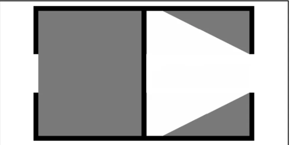
Figure 4-1: The Next Best Path Problem is NP-hard

Consider an occupancy map consisting pockets of unknown space (gray). Paths through free space (white) exist between these pockets but a direct line of sight is blocked by kinks. The unknown pockets and path kinks are enlarged for the pur-poses of visualization, but assume they are negligible compared to distances between pockets.

According to definition 2.5 a next best path will try to visit as many pockets as possible to maximize the its information gain. Therefore if a next best path with a bound 𝐷 on the total travel distance does not return a path between all pockets, a traveling salesman path [37] on the equivalent graph does not exist and vice versa.

Latombe [22]. At first glance this heuristic is ad hoc engineering, but by investi-gating its limits it is apparent that the heuristic effectively interpolates between two intuitive techniques; one detail oriented and the other anxious to keep moving. Based on the reasoning in §4.1, we claim this strategy works well in environments where un-known space is sparse.

The second heuristic studied in §4.3 is our own creation, constructed to perform well when the González-Banños and Latombe heuristic does not. This heuristic re-quires computing conditional mutual information. Since computing the conditional mutual information exactly is suspected to be hard [10], we provide efficient algo-rithms for computing upper and lower bounds in §4.4.

4.1

Justifying Nearest Neighbor Exploration

While real world environments are never as extreme as the one shown in figure 4-1, many still exhibit a nodal structure; there are a number of key locations that need to be visited to form a pretty complete map of the space. Leaving the formation of the set of key states to sections 4.2 and 4.3, the problem that remains to be solved is the traveling salesman problem.

Fortunately, the traveling salesman problem is a well studied problem with many polynomial time approximations schemes [4]. For example, if it is possible to compute travel costs between all states then one can construct a minimum spanning tree. Traversing this tree produces a path that is no more than twice the cost of the optimal path [4]. However, computing shortest paths between all pairs of states can be computationally expensive, especially for a system with nonlinear dynamics. One simple mantra requires computing shortest paths from only the current location: move to the nearest neighbor.

Traveling to the nearest neighbor is the oldest proposed heuristic for the traveling salesman problem [39]. In a graph satisfying the triangle inequality the heuristic in worst case produces a path that is Ω(log_{|𝑉 |) times the optimal path length where} |𝑉 | is the number of states [38]. But when planar graphs are random rather than adverserially constructed, the nearest neighbor path is on average only 25% longer than the length of the optimal path [25].

The cost functions of real systems may in fact be approximately planar if the robot has well behaved dynamics and navigates in a sparse 2D environment. Other scenarios involving strange system dynamics, maze-like obstacles, and travel in 3D may not obey this property. Still, we conjecture that in most practical cases the nearest neighbor path is on average not much worse than the optimal path.

4.2

The González-Baños and Latombe Heuristic

The González-Baños and Latombe heuristic [22] states that the next best path is the shortest path to the state maximizing

(x, Θ)* = arg max

x,Θ

exp(_{−𝜂𝑑(x, Θ))𝐼(𝑀; 𝑍}x,Θ) (4.1)

where 𝑑(x, Θ) is cost of the shortest path to state (x, Θ) and 𝜂 ≥ 0 is an algorithm parameter. The original presentation of the heuristic is brief, so here we give a more extended explanation of why and when it works.

A clear benefit of this heuristic is that it is easy to compute. One application of algorithm 1 produces 𝐼(𝑀 ; 𝑍x,Θ) for all cells x and all Θ by the advice of

re-mark 3.3. One application of a single source shortest path algorithm like Dijkstra’s algorithm [14] or RRT* [27] produces 𝑑(x, Θ) for all x and Θ.

To evaluate the heuristic’s performance at solving the next best path problem we consider a limiting case. When 𝜂 is large, equation (4.1) returns the nearest state with nonzero information. This is because the exponential term prioritizing nearby states dominates the mutual information term so long as the mutual information is nonzero.

Fitting this case to the template described in §4.1, it equivalently chooses all states with nonzero mutual information to be the key states that need to be visited and then applies a nearest neighbor strategy. In maps where range measurements made at opposing locations have overlapping views of unknown space then this set of states dramatically overestimates the actual sets of states that, when visited, form a complete map of the environment. But if unknown regions are small and occluded from each other the divergence between the sets decreases and the heuristic becomes a good fit.

The limiting case is also similar to frontier exploration [43]. But rather than moving to the nearest frontier, the heuristic declares the robot should move to the nearest state where a frontier is visible. This small change has the potential to save the cost of moving all the way to a frontier that turns out to be occupied by instead

viewing that frontier from a distance.

In practice the limiting case is not useful because in a noisy system the mutual information will never be exactly zero and so the robot will never move. Plus, like frontier exploration the heuristic is detail-oriented; a large𝜂 leads a robot to continue to tour one area of the map until it is entirely explored before moving on. This is desirable if the goal is to form a complete map of the entire space but not if the goal is to form a pretty good map of the space at lower cost.

Choosing a smaller 𝜂 smooths out both of these problems by mixing the exacting behavior with a restless one. In particular when 𝜂 = 0 the heuristic chooses to move to the next best view state; the robot will greedily travel to the most informative parts of the map disregarding travel distance.

4.3

A Conditional Heuristic

We claimed in §4.2 that the González-Baños and Latombe Heuristic works best when the set of states with nonzero mutual information is similar to the possible sets of states that, when visited, form a complete map of the environment. This requisite does not hold when measurements made in differing locations have a large dependence on each other.

This is why we propose another heuristic that takes the dependence between different measurements into account when forming a set of key states. Once this set is formed the nearest neighbor approach defended in §4.1 is applied to choose the best state to travel to.

This heuristic works by greedily choosing the most informative states one by one and for each choice accounting for its dependence on all previous choices. Specifically, choose the maximum over all x and Θ of 𝐼(𝑀 ; 𝑍x,Θ), i.e. the next best view. Then

choose the maximum over all x and Θ of 𝐼(𝑀 ; 𝑍x,Θ) conditioned on a measurement

made at the first location. Then choose the maximum conditioned on a measurement made at the first and second locations. Etc. The algorithm terminates when the maximizing mutual information is less than a factor 𝑒−𝜂 _{of next best view’s mutual}