HAL Id: inserm-00939284
https://www.hal.inserm.fr/inserm-00939284
Submitted on 24 Oct 2014
HAL is a multi-disciplinary open access
archive for the deposit and dissemination of
sci-entific research documents, whether they are
pub-lished or not. The documents may come from
teaching and research institutions in France or
abroad, or from public or private research centers.
L’archive ouverte pluridisciplinaire HAL, est
destinée au dépôt et à la diffusion de documents
scientifiques de niveau recherche, publiés ou non,
émanant des établissements d’enseignement et de
recherche français ou étrangers, des laboratoires
publics ou privés.
Evaluation of bootstrap methods for estimating
uncertainty of parameters in nonlinear mixed-effects
models: a simulation study in population
pharmacokinetics
Hoai-Thu Thai, France Mentré, Nick Holford, Christine Veyrat-Follet,
Emmanuelle Comets
To cite this version:
Hoai-Thu Thai, France Mentré, Nick Holford, Christine Veyrat-Follet, Emmanuelle Comets.
Evalua-tion of bootstrap methods for estimating uncertainty of parameters in nonlinear mixed-effects models:
a simulation study in population pharmacokinetics. Journal of Pharmacokinetics and
Pharmacody-namics, Springer Verlag, 2014, 41 (1), pp.15 - 33. �10.1007/s10928-013-9343-z�. �inserm-00939284�
(will be inserted by the editor)
Evaluation of bootstrap methods for estimating uncertainty of parameters
in nonlinear mixed-effects models: a simulation study in population
pharmacokinetics
Hoai-Thu Thai · France Mentré · Nicholas H.G. Holford · Christine Veyrat-Follet · Emmanuelle Comets
Received: date / Accepted: date
Abstract Bootstrap methods are used in many disciplines to estimate the uncertainty of parameters, in-cluding multi-level or linear mixed-effects models. Residual-based bootstrap methods which resample both random effects and residuals are an alternative approach to case bootstrap, which resamples the individuals. Most PKPD applications use the case bootstrap, for which software is available. In this study, we evaluated the performance of three bootstrap methods (case bootstrap, nonparametric residual bootstrap and para-metric bootstrap) by a simulation study and compared them to that of an asymptotic method in estimating uncertainty of parameters in nonlinear mixed-effects models (NLMEM) with heteroscedastic error. This simulation was conducted using as an example of the PK model for aflibercept, an anti-angiogenic drug. As expected, we found that the bootstrap methods provided better estimates of uncertainty for parameters in NLMEM with high nonlinearity and having balanced designs compared to the asymptotic method, as implemented in MONOLIX. Overall, the parametric bootstrap performed better than the case bootstrap as the true model and variance distribution were used. However, the case bootstrap is faster and simpler as it makes no assumptions on the model and preserves both between subject and residual variability in one resampling step. The performance of the nonparametric residual bootstrap was found to be limited when ap-plying to NLMEM due to its failure to reflate the variance before resampling in unbalanced designs where the asymptotic method and the parametric bootstrap performed well and better than case bootstrap even with stratification.
Keywords Bootstrap· Nonlinear mixed-effects models · Pharmacokinetics · Uncertainty of parameters ·
MONOLIX
1 Introduction
Nonlinear mixed-effects models (NLMEM) have been widely used in the field of pharmacokinetics (PK) and pharmacodynamics (PD) to characterize the profile of drug concentrations or treatment response over time for a population. NLMEM not only provides the estimates of fixed-effect parameters in the studied population but also describes their variability quantified by the variance of the random effects in a single estimation step. This approach was introduced by Lewis Sheiner and Stuart Beal and has now become an
H.T. Thai · E. Comets · F. Mentré
INSERM, UMR 738, F-75018 Paris, France; Univ Paris Diderot, Sorbonne Paris Cité, UMR 738, F-75018 Paris, France E-mail: [email protected]
N.H.G. Holford
Department of Pharmacology and Clinical Pharmacology, University of Auckland, Auckland, New Zealand H.T. Thai · C. Veyrat-Follet
integral part of drug development since the first application of NLMEM in population PKPD in the late 1970s [1]. The parameters of NLMEM are often estimated by the maximum likelihood (ML) method.
These models are complex, not only structurally but also statistically, with a number of assumptions about the model structure and variability distributions. The uncertainty of parameters in NLMEM is usu-ally quantified by the standard errors (SE) obtained asymptoticusu-ally by the inverse of the Fisher information
matrix (MF) and by the asymptotic confidence intervals (CI) which are assumed to be normal and
symmet-ric. However, this uncertainty might be biased when the assumption of asymptotic normality for parameter estimates and their SE is incorrect, for example when the sample-size is small or the model is more than trivially nonlinear. Sometimes, they cannot be even obtained due to the over-parameterization of the model
or numerical problems when evaluating the inverse of the MF.
The bootstrap is an alternative method to assess the uncertainty of parameters without making strong distributional assumptions. It was first introduced by Efron (1979) for independent and identically dis-tributed (iid) observations. The principal idea behind the bootstrap is to repeatedly resample the observed data with replacement to create new datasets having the same size as the original dataset, then fit each boot-strap dataset to construct the distribution of an estimator or a statistic of interest [2, 3]. In standard linear regression, the most simple and intuitive method is the case bootstrap which consists of resampling the pairs of observations with replacement. However, other bootstrap methods exist; for example the residual bootstrap and the parametric bootstrap [4, 5, 6, 7]. The residual bootstrap resamples the observed residuals obtained after model fitting then constructs the bootstrap samples. The parametric bootstrap adopts the prin-ciple of the residual bootstrap but simulates the residuals from the estimated distribution obtained by the fitting of the original data, e.g the normal distribution. In the mixed-effects models setting, the case boot-strap consists of resampling the whole vector of observations in one subject with replacement. Classical bootstrap methods used in linear regression with just one level of variability have been extended to take into account the characteristics of mixed-effects models with two levels of variability (between-subject and residual variability) [8]. Resampling random effects was proposed to be coupled with resampling residuals [8, 9, 10, 11].
In a previous study [12], we conducted a simulation study to evaluate different bootstrap methods that could be used for linear mixed-effects models (LMEM) with homoscedastic residual error, a simple case before moving to NLMEM. The study demonstrated the adequate performance of the nonparamet-ric/parametric random effect and residual bootstrap which resamples directly two levels of variability and the case bootstrap which is considered to preserve both of them in all evaluated designs. On the other hand, the bootstrap methods which resample only the residuals performed poorly with a large underestimation of the SE of parameters and poor estimates of coverage rates. This is because the between-subject variability of parameters in the evaluated designs were not taken into account. The worse performance was also ob-tained for the bootstraps combining case and residual, in which the residual variability is considered already resampled in the case bootstrap.
In order to understand the use of bootstrap in the field of population PKPD, we conducted a literature re-search in PUBMED with the keywords "bootstrap AND population AND (pharmacokinetics OR pharmaco-dynamics OR pharmacokinetic-pharmacodynamic OR pharmacokinetic/pharmacodynamic) AND (NON-MEM OR MONOLIX OR nonlinear mixed effects)" and recovered 90 papers up to November 2012. All of them used the case bootstrap as a model evaluation tool, and only one of them used the parametric bootstrap, as a complement to the case bootstrap. The purpose of using bootstrap in PKPD was mainly for comparing the parameter estimates obtained from the bootstrap datasets with those obtained in the original dataset and estimating SE and/or constructing CI (in 90% papers). It was less frequently used for covariate selection (in 6.7% papers) and structural model selection (in 3.3% papers). Both nonparametric case bootstrap and para-metric bootstrap are implemented in programs, Wings for NONMEM and Pearl-speaks-NONMEM (PsN) [13, 14]. While the case bootstrap has been mostly used in population PKPD, there have been very few stud-ies in the literature to evaluate its performance, especially in comparison with the nonparametric/parametric random effect and residual bootstrap which may better approach the "true" data generating process.
In the present paper, we evaluated the performance of different bootstrap methods by a simulation study and compared them to that of the asymptotic method in estimating uncertainty of parameters in NLMEM with heteroscedastic error. This simulation design was based on real PK data collected from two clinical trials of aflibercept, an anti-VEGF drug, in cancer patients.
2 METHODS 2.1 Statistical models
Letyijdenote the observationj of subject i at time tij, wherei = 1, ..., N ; j = 1, ..., ni, yi = (yi1, yi2, ..., yini)
T
regroups the (ni×1) vector of measurements in subject i, ξi= (ti1, ti2, ..., tini)
T
presents the design vector
of subjecti, y = (y1, ..., yN) regroups all the measurements from N subjects, ntot=∑Ni=1nidenotes the
total number of observations. We define an NLMEM as follows: yi= f (ξi, ϕi) + g(ξi, ϕi, σ)ϵi ϕi= h(µ, ηi) ηi∼ N (0, Ω) ϵi∼ N (0, 1) (1)
wheref is the structural model, g is the residual error model, σ is the vector of parameters in the residual
error model, ϵi= (ϵi1, ..., ϵini) are standardized errors which are normally distributed with mean zero and
variance 1, ϕiis the (p×1) vector of individual regression parameters, µ is the (p×1) vector of fixed effects,
h is the function of individual parameters ϕi, ηiis the (q × 1) vector containing the random effects and Ω
is the (q × q) covariance matrix of the random effects. The random effects ηiand the residual errors ϵiare
assumed to be independent for different subjects and to be independent of each other for the same subject.
The individual PK parameters are often assumed to follow log-normal distribution ϕi = µ exp(ηi). Special
cases forg include g = σa(constant/homoscedastic error model) andg = σpf (ξi, ϕi) (proportional error
model).
2.2 Estimation methods
The parameters of NLMEM are estimated by maximizing the log-likelihood functionL(y|θ) of the response
y, with θ = (µ, Ω, σ) the (l × 1) vector of all parameters of the model. This function is given by:
L(y|θ) = N ∑ i=1 L(yi|θ) = N ∑ i=1 log (∫ p(yi, ϕi; θ)dϕi ) = N ∑ i=1 log (∫ p(yi|ϕi; θ)p(ϕi; θ)dϕi ) (2)
wherep(yi|ϕi; θ) is the conditional density of the observations given the random effects, p(ϕi; θ) is
the density of the individual parameters andp(yi, ϕi; θ) is the likelihood of the complete data (yi, ϕi) of
subjecti.
As the random effects are unobservable and the regression function is nonlinear, the likelihood of NLMEM has no closed form and cannot be evaluated analytically. The likelihood is usually approximated
by linearisation of the functionf , such as First Order (FO) and First Order Conditional Estimation (FOCE)
methods implemented in NONMEM [15]. These methods linearise the structural model either around the expectation of the random effects (FO) or around the individual predictions of the random effects (FOCE). Although the linearisation methods are numerically efficient, they have the potential of producing inconsis-tent estimates when the between-subject variability is high [16, 17]. An alternative method to linearisation is to use the Stochastic Approximation Expectation-Maximization (SAEM) algorithm as an exact ML com-putation [18]. This algorithm consists, at each iteration, in successively simulating the random effects with the conditional distribution (E step) using Markov Chain Monte-Carlo procedure and updating the unknown parameters of the model (M step). In this simulation study, we used the SAEM algorithm implemented in MONOLIX 4.1.2 (Matlab version) as the estimation method.
The ML estimate ˆθ of θ is asymptotically normally distributed with mean θ and asymptotic
estima-tion covariance matrix given by the inverse of MF. MF is computed as the negative Hessian of the
log-likelihood in all the model parameters:
MF= N ∑ i=1 −∂2L(y i|θ) ∂θ∂θ′
As the likelihood has no closed form, a linearisation of the model around the conditional expectation
of the individual Gaussian parameters has been proposed to derive an approximate expression of the MF,
computed as the expectancy of the derivative of minus twice the log-likelihood with respect to the
parame-ters. This approach is implemented in MONOLIX where the MFof this Gaussian model is a block matrix
with no correlations between estimated fixed-effects and the estimated variances. The gradient off is
nu-merically computed. This method, called MFby linearisation, was used in this simulation study to calculate
the SE of parameters.
The asymptotic SE of parameters are then estimated as the square root of the diagonal element of the estimated covariance matrix.
When the parameters of the model have been estimated, empirical Bayes estimates (EBEs) of the
indi-vidual parameters ϕican be obtained as the mode of the posterior distribution of ϕi:
m(ϕi|yi; ˆθ) = Argmaxφip(ϕi|yi; ˆθ)
2.3 Bootstrap methods
The principle of the bootstrap is to repeatedly generate pseudo datasets by resampling with replacement from the original sample. The unknown original distribution of parameters may be replaced by the empirical distribution of the sample, which refers to the nonparametric bootstrap [19] or simulated from a parametric distribution, which refers to the parametric bootstrap. In this study, we are interested in bootstrap methods in regression.
Let B be the number of bootstrap samples to be drawn from the original dataset, a general bootstrap algorithm in regression is:
1. Generate a bootstrap sample by resampling from the data and/or from the estimated model 2. Obtain the estimates for all parameters of the model for the bootstrap sample
3. Repeat steps 1 & 2 B times to obtain the bootstrap distribution of parameter estimates and then compute mean, standard deviation, and 95% CI of this distribution as described below
Let ˆθ∗
b be the vector of parameters estimated for thebthbootstrap sample. The bootstrap parameter
estimate ˆθBis calculated as the median of the parameter estimates from the B bootstrap samples.
The bootstrap standard error of thelthcomponent of ˆθ
B is obtained as the standard deviation of the
estimated parameters from the B bootstrap samples:
c SE(l)B = v u u t 1 B − 1 B ∑ b=1 (ˆθ∗(l) b − ˆθ (l) B )2 (3)
A 95% bootstrap confidence interval of thelthcomponent ofθ can be constructed by calculating the
2.5thand 97.5thpercentiles of the bootstrap distribution. The bootstrap samples are first sorted into
ascend-ing order and these percentiles are respectively given by the(B + 1)αthand(B + 1)(1 − α)thelements of
the ordered bootstrap samples whereα=0.025. When (B + 1)α does not equal a whole number,
An alternative approach is to use a normal approximation to construct a bootstrap confidence interval
(CI), using the estimated cSEB:
[ˆθ(l)B − cSE (l) B · z1−α/2; ˆθ (l) B + cSE (l) B · z1−α/2] (4)
z1−α/2denotes the1 − α/2 quantile of the standard normal distribution (z0.975 = 1.96). However, it is
preferable to use bootstrap percentile CI rather than the normal approximation CI using the bootstrap SD. [5, 20]. In this study, we used empirical percentiles, but other methods dealing with skewed distributions, such as the bias-corrected percentile method [5], could also be investigated.
In the present study, we evaluated the three bootstrap methods which showed a good performance in
LMEM [12]: the case bootstrap Bcase, the nonparametric bootstrap of random effects and global residuals
Bη,GRand the parametric bootstrap BPη,PR. The individual residual bootstrap was not evaluated in this
study because this method appeared not to be consistent with the non-correlated structure of residuals, although it had provided similar results to the global residual bootstraps in the LMEM. All the bootstrap methods which did not perform well in LMEM were not evaluated in this NLMEM study.
The detailed algorithms of the evaluated bootstrap methods to obtain a bootstrap sample (bootstrap generating process) are presented below.
2.3.1 Case bootstrap (Bcase)
This method consists of resampling with replacement the entire subjects, that is the joint vector of design
variables and corresponding responses (ξi, yi) from the original data before modeling. It is also called the
paired bootstrap. It is the most obvious way to do bootstrapping and makes no assumptions on the model.
2.3.2 Nonparametric random effect and residual bootstrap (Bη,GR)
This method consists of resampling with replacement the random effects obtained after model fitting, as well as the residuals globally. The bootstrap sample is obtained as follows:
1. Fit the model to the data then estimate the random effectsηˆifrom { ˆϕi} and the standardized residuals
ˆ
ϵij = (yi− f (tij, ˆϕi))/g(tij, ˆϕi, ˆσ)
2. Draw a sample {η∗
i} of sizeN with replacement from { ˆηi} by assigning an equal probabilityN1 to each
value
3. Draw a sample {ϵ∗}={ˆϵi∗j∗} of sizentotwith replacement globally from {ˆϵij}
4. Generate the bootstrap responses y∗
i = f (ξi, ˆµ, η∗i) + g(ξi, ˆµ, η∗i, ˆσ)ϵ∗i
Note that in mixed-effects modeling, the raw random effects and residuals do not necessarily have a zero mean, and their variance/ covariance matrix does not match the model-estimated residual vari-ance/covariance matrices. That’s why the nonparametric bootstrap of the raw residuals yields downwardly biased variance parameter estimates [5, 6, 21]. Therefore, they both must be rescaled by being centred and then transformed to have empirical variance/covariance matrices equal to those estimated by the model. In linear mixed-effects models, Carpenter et al. proposed to center the random effects and residuals and then transform them using correction matrices accounting for the differences between their corresponding estimated and empirical variance-covariance matrices (shrinkage) [21, 22]. The correction matrices were calculated using the Cholesky decomposition of both estimated and empirical variance-covariance matri-ces.
In this study, we extended the correction of Carpenter et al. for NLMEM by using Eigen Value De-composition (EVD), a special case of Singular Value DeDe-composition (SVD) for square symmetric matrices [23], instead of the Cholesky decomposition. This extension was done to deal with the numeric problems sometimes seen in nonlinear models where some eigenvalues of the variance-covariance matrix are very close to zero. The detailed transformation of random effects and residuals is presented in Appendix.
2.3.3 Parametric random effect and residual bootstrap (BPη,PR)
This method resamples both random effects and residuals by simulating from the estimated distributions after model fitting. The bootstrap sample is obtained as follows:
1. Fit the model to the data
2. Draw a sample {η∗
i} of sizeN from a multivariate normal distribution with mean zero and covariance
matrix ˆΩ
3. DrawN samples {ϵ∗
i} of sizenifrom a normal distribution with mean zero and variance one
4. Generate the bootstrap responses y∗
i = f (ξi, ˆµ, η∗i) + g(ξi, ˆµ, η∗i, ˆσ)ϵ∗i
Of note that, the simulation of random effects from a multivariate normal distribution can raise problem
when ˆΩ contains one or some eigenvalues close to zero. We proposed to construct pseudo matrix of ˆΩ using
EVD: ˆΩ′ = V
ˆ
ΩDΩˆ′VΩˆ
T
whereVΩˆ is the orthogonal matrix resulting from EVD of ˆΩ, DΩˆ′is the diagonal
matrix containing eigenvalues of ˆΩ in diagonal entries, of which eigenvalues smaller than a tolerance (10−6)
was set to zero.
2.4 Bootstrap methods with stratification
The nonparametric bootstrap methods described above preserve the structure and the characteristics of the original data when the data is homogenous. In the case of unbalanced designs, different groups in the original data should be defined and resampling in each group should be done to maintain a similar structure of the original data in the bootstrap sample [14]. For example when a study includes different numbers of observations in each subject, the case bootstrap will generate the bootstrap samples having different total number of observations. The nonparametric residual bootstrap preserves the same structure of the original data but does not take in to account the different shrinkages of random effects and residuals for groups with different designs. Bootstrap with stratification can be done for these two methods in this example as follows:
Case stratified bootstrap(Bstrat
case). This method consists in resampling the entire subjects in each group.
Nonparametric residual stratified bootstrap (Bstratη,GR). This method applies the correction for
shrink-age and bootstrapping the random effects and the residuals separately in each group. An example of the correction for shrinkage with two data groups with different designs is presented in Appendix.
3 SIMULATION STUDIES 3.1 Motivating example
As an illustrative example, data from two clinical trials of aflibercept, an anti-angiogenic drug for cancer patients were used. The first trial was a phase I dose-escalation study of aflibercept in combination with docetaxel and cisplatin in patients with advanced solid tumors [24]. The second trial was a randomised con-trolled phase III study of aflibercept and docetaxel versus docetaxel alone after platinum failure in patients with advanced or metastatic non-small-cell lung cancer [25]. Aflibercept was administered intravenously every 3 weeks in combination with docetaxel at dose levels ranging from 2 to 9 mg/kg in the phase I trial and at dose of 6 mg/kg in the phase III trial. In the phase I trial, blood samples were collected at 1, 2, 4, 8, 24, 48, 168, 336 hours after the start of aflibercept administration and before the administration of all subsequent cycles. In the second trial, blood samples were taken pre-dose and at the end of aflibercept infu-sion on day 1 (cycle 1) and every odd cycles before treatment administration and at approximately 30 and 90 days after the last aflibercept treatment. The free plasma aflibercept concentrations were measured in all samples using enzyme-linked immunosorbent assay (ELISA) method. The limit of quantification (LOQ) for free aflibercept in plasma was 15.6 ng/ml and data below LOQ for both studies (6.3% for the phase I trial and 9.1% for the phase III trial) were omitted.
For this simulation study, we focused mainly on the data after the first dose of the phase I trial and the data after the two first doses of the phase III trial disregarding potential interoccasion variability. All the patients having at least two observations were included in this analysis. This subset contains 344 patients including 53 patients from the phase I trial with an average of 9 observations per patient (rich design group) and 291 patients from the phase III trial with 2 observations per patient (sparse design group).
To describe the PK of free aflibercept, we analysed jointly the data of all patients using MONOLIX 4.1.2 (Matlab version) and the SAEM algorithm for estimating parameters. A two-compartment infusion PK model with first-order linear elimination described the aflibercept concentrations in this subset. The between-subject variability was modeled using an exponential model. The residual variability was chosen among the additive, proportional or combined models using the log-likelihood (LL) test. We examined the SAEM convergence graph and the goodness-of-fit plots to evaluate the chosen model.
The proportional error model was the best residual model. With respect to the model of random effects,
there was a high correlation betweenCL and Q (0.9), which decreased 47 point in -2LL, compared to
the model without this correlation. The variability ofV2was small so it was fixed to zero to have a better
convergence of parameters. This did not change significantly the log-likelihood. The parameter estimates of this model are presented in first column of Table 3. All the parameters were estimated with good precision
(RSE < 15%) obtained by the asymptotic MF method. With the chosen model, the goodness-of-fit was
satisfactory.
3.2 Simulation settings
In this simulation, we aimed to evaluate the performance of bootstrap in different designs using the first-order elimination PK model and their parameter estimates developed in the real data (section 3.1): a frequent sampling design, a sparse sampling design and an unbalanced design with mixing of the frequent and the sparse observation designs during resampling. We also aimed to evaluate the bootstraps in models with higher nonlinearity; a mixed-order (Michaelis-Menten) elimination model was used to illustrate this case.
For the balanced designs, the sampling times were identical for all subjects.
First-order elimination frequent sampling design. We simulated N=30 subjects with n=9 observations per subject at 1, 2, 4, 8, 24, 48, 168, 336, 503 hours after administration of aflibercept. In this design, we
used the same model developed for the real data, except for a smaller correlation betweenCL and Q (0.5
instead of 0.9) to avoid the convergence problems.
First-order elimination sparse sampling design. We simulated N=70 subjects with n=4 observations per subject at 1, 24, 48, 503 hours after administration of aflibercept. These 4 sampling times were selected among those in the frequent sampling design using D-optimality with PFIM software [26]. In this design,
we removed the correlation betweenCL and Q as well as the variability for Q (which created convergence
problems) and the variability onV2could then be estimated. The variability of other parameters was set to
30%.
Mixed-order (Michaelis-Menten) elimination frequent sampling design. We simulated N=30 subjects with n=9 observations per subject at 1, 2, 4, 8, 24, 48, 168, 336, 503 hours after administration of aflibercept. In this design, we used the same model of the linear sparse design but replaced first-order elimination
(CL=0.04 (l/h)) by mixed-order elimination (Vmax=2 (mg/h) with ωVmax=30% and Km=20 mg/l with
ωKm=0%) to increase the nonlinearity of the model. The values ofVmaxandKmwere chosen based on the
changes in the partial derivatives with respect to these parameters, to increase nonlinearity of the function f while providing similar concentration profiles compared with those in the first-order frequent design.
For the unbalanced design, we used the first-order elimination model in the sparse balanced design and
simulated two groups of patients:N1=15 withn1=9 observations per subject at 1, 2, 4, 8, 24, 48, 168, 336,
503 hours after administration of aflibercept, andN2=75 withn2=2 observations per subject at 1, 503 hours
after administration of aflibercept. The ratio of patients with frequent and sparse sampling was similar to that in the real data (16.7% subjects have rich sampling times with an average of 9 observations and 83.3% subjects have only 2 observations).
For each design, we simulated K=100 replications. The SAEM algorithm implemented in the MONO-LIX 4.1.2 was used to fit the data. The fixed-effects parameters were estimated with no transformation and the variability terms were estimated as standard deviations (SD). The asymptotic SE of parameters were
obtained by the inverse of MF, computed as the negative Hessian of log-likelihood (described previously
in Methods section). The bootstrap algorithms were implemented inR 2.14.1. All the bootstrap datasets
were fitted with the initial values obtained from estimates from the original data. Examples of simulated data for each given design are illustrated in Figure 1.
3.3 Evaluation of bootstrap methods
We drew B= 999 bootstrap samples for each replication of simulated data and for each bootstrap method. B=999 was chosen to directly estimate the quantiles for 95% CI without interpolation [5, 20]. For each
method, we therefore performed 99900 fits (100 simulated datasets× 999 bootstrap datasets).
For thekthsimulated dataset and for a given bootstrap method, we computed the bootstrap parameter
estimate ˆθB;k(l) as the median of parameter estimates from 999 bootstrap samples, and the bootstrap SE
estimate cSE(l)B;k as in equation (3) as well the CI, for thelthcomponent ofθ. The relative bootstrap bias
(RBBias) of thelthcomponent of bootstrap estimate ˆθ
Bwas obtained by comparing the bootstrap estimate
ˆ
θ(l)B;kand the estimate ˆθ
(l) k as follows: RBBias(ˆθ(l)B ) = 1 K K ∑ k=1 ( ˆθ(l)B;k− ˆθ (l) k ˆ θk(l) × 100 ) (5)
The average bootstrap SE was obtained by averaging the SE from equation (3) over the K=100 datasets. The true SE is unknown, but we can get an empirical estimate from the standard deviation of the estimated parameters over the K simulated datasets:
d SE(l)empirical= v u u t 1 K − 1 K ∑ k=1 (ˆθk(l)−θ¯ˆ(l))2 (6)
where¯ˆθ(l)is the mean of K values for thelthcomponent of the estimate ˆθ.
The relative bias (RBias) on SE of thelthcomponent of ˆθ
Bwas then obtained by comparing the average
SE to the empirical SE:
RBias(dSE(l)B ) = 1 K ∑K k=1dSE (l) B;k− dSE (l) empirical d SE(l)empirical × 100 (7)
The coverage rate of the 95% bootstrap confidence interval (CI) was defined as the percentage of the K=100 datasets in which the bootstrap CI contains the true value of the parameter.
The bootstrap approaches were compared in terms of the Rbias on the bootstrap parameter estimates, the Rbias on SE, and the coverage rate of the 95% CI of all parameter estimates from all bootstrap samples. The performance of the bootstrap methods were also compared to the performance of the asymptotic method (Asym) in terms of the Rbias on SE and the coverage rate of the 95% CI. The relative bias of asymptotic
SE estimate was defined in the same way as equation (7), but with respect to dSE(l)k being the asymptotic
SE of ˆθk(l)instead of dSE(l)B;k. The coverage rate of the 95% asymptotic CI was defined as the percentage of
datasets in which the asymptotic CI contains the true value of the parameter.
The relative estimation bias (REBias) of thelthcomponent of the estimate ˆθ was obtained by comparing
REBias(ˆθ(l)) = 1 K K ∑ k=1 ( ˆθ(l) k − θ (l) 0 θ(l)0 × 100 ) (8)
The bootstrap parameters estimates and their SE were defined as unbiased when relative bias was within ±10%, moderately biased (relative bias from ±10% to ±20%) or strongly biased (relative bias > ±20%).
The coverage rate of the 95% CI was considered to be good (from90% to 100%), low (from 80% to 90%) or
poor (< 80%). A good bootstrap was defined as a method providing unbiased estimates for the parameters and their corresponding SE, and ensuring a good coverage rate of the 95% CI. The same criteria were used to evaluate the performance of the asymptotic method.
3.4 Application to real data
All the bootstrap methods evaluated in the simulations studies were then applied to the real data with B=999 replications. The parameter and SE estimates obtained by the bootstrap methods were compared to those obtained by the asymptotic approach.
4 RESULTS
4.1 Simulation studies
Performance of bootstrap in balanced designs
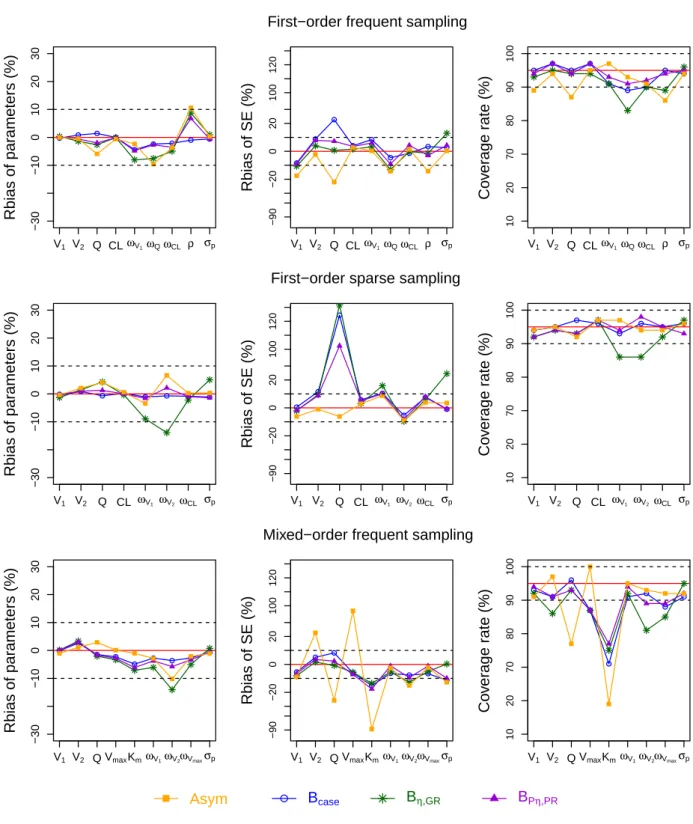
The performance of the three bootstrap methods as well as the asymptotic method regarding the relative bias of parameters, their SE and the coverage rate of 95% CI are presented in Figure 2 and Table 1. In the frequent sampling setting with first-order elimination, all bootstrap methods showed essentially no bias
for all parameters. In terms of SE estimation, the case bootstrap (Bcase) yielded moderate bias for SE of
Q (22.1%); the nonparametric random effect and residual bootstrap (Bη,GR) showed a small bias for SE
ofωQ andσp (< 13.2%) while the parametric random effect and residual bootstrap (BPη,PR) estimated
correctly all the SE. In terms of coverage rate, all the bootstrap methods provide good coverage rate for
all parameters, except for low coverage rate of the correlation betweenCL and Q (ρ) (83%) observed for
Bη,GR. The asymptotic method performed however less well than the bootstrap methods with a greater bias
for SE of several parameters (V1,Q, ωQ,ρ) and poorer coverage rates for V1,Q, and ρ.
In the first-order elimination sparse sampling setting where the correlation betweenCL and Q was
omitted and the variability of parameters was set to 30%, the Bcase and the BPη,PR showed no bias in
parameter estimates, SE and provided good coverage rates for all parameters except for a large bias for SE
ofQ (> 100%). The Bη,GRnot only provided large bias for SE ofQ, but also gave a bias for SE of ωV1
andσ and poor coverage rates for ωV1andωV2. The asymptotic method, however, performed very well and
better than the bootstrap methods.
Higher nonlinearity was evaluated in the mixed-order elimination frequent sampling setting. In this
design, all bootstrap methods estimate correctly all the parameters except for a moderate bias onωV2
ob-served for Bη,GR. In terms of SE estimation, the bootstrap methods provided good estimates for the SE
of all parameters, with the exception for underestimation of SE ofKmobserved for all methods (-17.6 to
-13.6%). In addition, the Bcaseunderestimated SE ofσpand Bη,GRunderestimated SE ofωV2. In terms of
coverage rate, the bootstrap methods provided good coverage rates for first-order elimination parameters
but gave poor to low coverage rates for more highly nonlinear parameters (87% forVmaxand 71-77% for
Km). Compared to the bootstrap methods, the asymptotic method showed higher bias for SE of almost all
parameters, especially for nonlinear parameters, e.gKm(-89.3%); which leads to extremely poor coverage
rate forKm(19%). However, the CI of Km was very narrow and distance from the CI to the true value was
small across all the simulated data. This bias may therefore be considered as negligible in practical terms.
The boxplots of the relative error of SE of all parameter estimates obtained by the bootstrap methods and the asymptotic method in all evaluated designs are shown in Figure 3. The range of relative errors of boot-strap SE across the K=100 replications did not show any practically relevant differences across the bootboot-strap methods. The range of relative errors was however different between the asymptotic method and the boot-strap methods. In the sparse sampling design, the estimates of SE obtained by the asymptotic method were
more accurate and precise, especially forQ. On the contrary, the asymptotic method performed less well
than the bootstrap methods in frequent sampling designs with underestimation of SE of several parameters,
especially SE ofKmin the mixed-order design where SE ofV2andVmaxwere also overestimated.
Performance of bootstrap in the unbalanced design
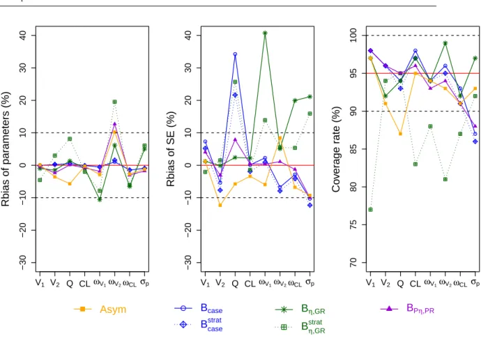
In the fourth simulation setting, we considered a highly unbalanced design where 16.7% subjects have rich sampling times with average 9 observations and 83.3% subjects have only 2 observations. Figure 4 and Table 2 present the results of the bootstrap methods with and without stratification and the asymptotic method in this simulation. All the non-stratified bootstrap methods estimated correctly the parameters,
ex-cept for a slight overestimation ofωV2observed in the BPη,PR. In terms of SE estimation, the case bootstrap
did not estimate well the SE ofQ with a bias of 34.3%; there were also a high bias on SE of ωV1(40.8%),
ωCL (20%),σp (21.1%) for the Bη,GR. In terms of coverage rates, the nonparametric bootstrap methods
provided overly wide CI (coverage rates over 97%) for the parameters whose SE were over-estimated,
ex-cept forωCL in the Bη,GR. The overly wide confidence intervals could be due to more extreme values in
the parameter estimates than expected for bootstrapped datasets because the 50% CI retained a reasonably good coverage rate (Table S1 in Appendix). On the other hand, the parametric bootstrap provided good
coverage rates for most parameters, except for overly wide CI for V1 and lower coverage rate ofσpwhich
was also seen in Bcase. The asymptotic method performed reasonably well in this unbalanced design with
only a small bias on SE ofV2and lower coverage rate ofQ.
The stratified bootstrap methods were also evaluated in this unbalanced design in order to maintain the
same structure of the original dataset. The stratified case bootstrap Bstratcase reduced the bias in SE ofQ but
this bias was still high (21.7 vs 34.3%). The stratified residual bootstrap Bstratη,GRreduced the bias in SE of
ωV1 andσpbut overestimated SE ofQ and gave lower coverage rates for almost all parameters compared
to the non-stratified version.
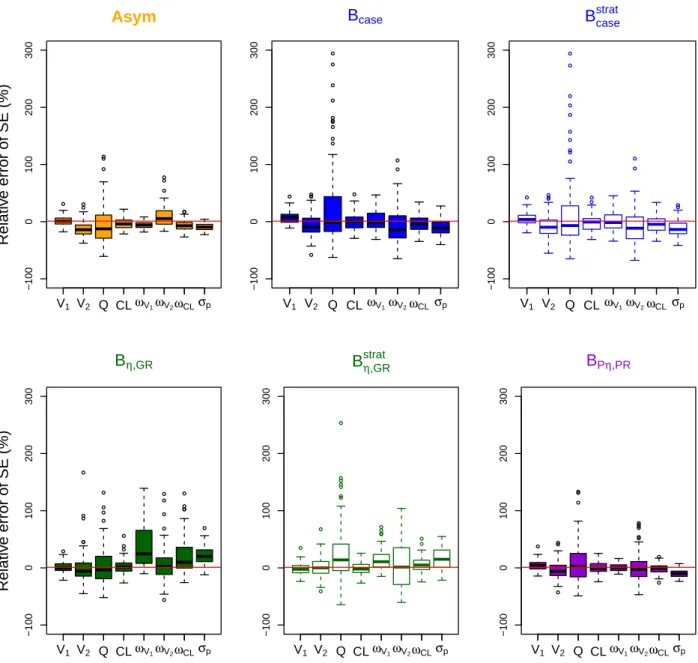
Figure 5 presents the boxplots of the relative error of SE of all parameter estimates obtained by the
bootstrap methods and the asymptotic method in the unbalanced design. The Bcase and Bstratcase estimated
with less precision the SE ofQ with a very large variability compared to other bootstrap methods. The
BPη,PRand the asymptotic method estimate most correctly and precisely the SE of all parameter estimates.
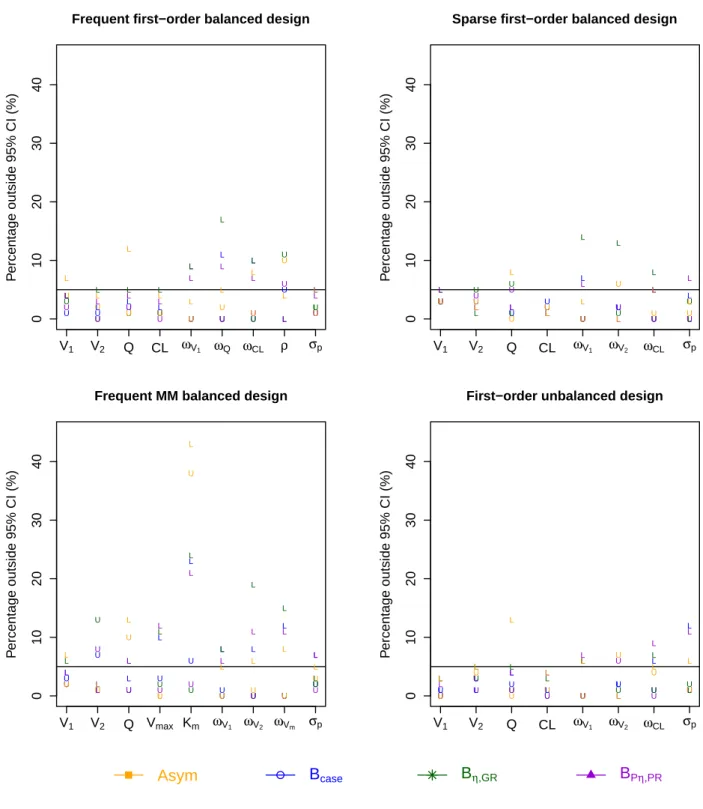
More information on whether the confidence intervals provided by the asymptotic method and the boot-strap methods (non-stratified version) missed on the lower (L) or upper (U) side of the true value for each
parameter and for 4 evaluated designs is shown in Figure S1 in Appendix. For theKmparameter in the
MM balanced design, the CI provided by the asymptotic method missed on both the lower and upper sides of the true value; while those of the bootstrap methods missed on the lower side.
Of note that, 100% simulated and bootstrap datasets converged in all evaluated designs.
4.2 Application to real data
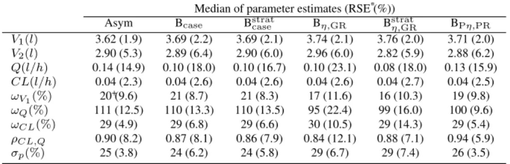
Table 3 presents the median of the parameter estimates obtained by the bootstrap methods for the real dataset and the bootstrap relative standard errors with respect to the original parameter estimates. We found
that all the bootstrap methods had similar medians of parameter estimates, except forQ with the difference
between BPη,PRand the other methods. In terms of precision estimation, the bootstrap methods provided
good RSE for all parameters (<24%). However, there were some differences for the estimation of RSE of
Q and variance parameters. Similar to the simulation results in the unbalanced design, Bη,GRand Bstratη,GR
gave higher RSE for the variance parameters compared to the other methods. The asymptotic method and
BPη,PRhad very similar estimates for almost all parameters in terms of both parameter and RSE estimation,
including RSE ofσpwhich was larger for other methods.
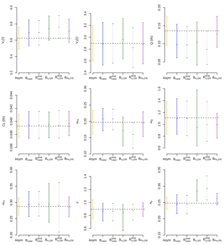
The bootstrap confidence intervals for each parameter are shown in Figure 6. The parameter estimates
which lay outside the CI of Bη,GRand Bstratη,GR. For Bstratη,GR, the estimates ofV1,Q, ωV1were located on the
boundary of the bootstrap CI. Compared to the asymptotic CI, the CI of Bcaseand Bstratcase for all parameters
were similar except forQ while the CI of Bη,GR and Bstratη,GR were different, especially for the stratified
version.
5 DISCUSSION
In the present paper, we evaluated the performance of the case bootstrap and the nonparametric/parametric bootstrap of random effects and residuals by a simulation study and compared them to that of the asymptotic method in estimating uncertainty of parameters in NLMEM with heteroscedastic error. This simulation was based on a real PK data collected from two clinical trials of aflibercept, a novel anti-angiogenic drug, in cancer patients.
When dealing with NMLEM, we should consider other factors which influence the bootstrap, such as the nonlinearity of the model and the heteroscedasticity. It should be noted that bootstrapping nonlinear models is done in the same manner as bootstrapping linear models. However, the nonlinearity makes the estimation process much more difficult and laborious. The bootstrap becomes time consuming because we need to perform a nonlinear estimation for each bootstrap sample. The complexity increases when the residual error model is heteroscedastic (the variance of residuals errors is not constant) because the residuals can not be interchangeable. The algorithm for bootstrapping the residuals will not be valid because the bootstrapped dataset might not have the same variance model as the original data. To overcome this issue, the residuals errors need to be standardized to have the same variance before bootstrapping [27]. However, heteroscedasticity is not a problem for the case bootstrap because heteroscedasticity will be preserved after bootstrapping.
Another issue which is very important when applying the nonparametric residual bootstrap in NLMEM is the transformation of the raw residuals to avoid the underestimation in variance parameter estimates [5, 6, 21]. The shrinkage correction using the ratio matrix between the empirical and the estimated variance covariance matrices was proposed by Carpenter et al., using the Cholesky decomposition for a positive definite matrix [21, 22]. This correction performed very well for LMEM [12]. In NLMEM, the numerical problems make the empirical and/or estimated variance-covariance matrices sometimes closer to a semi-positive definite matrix with one or several eigenvalues close to zero. We used the EVD, a special case of SVD for square symmetric matrices [23], to obtain the ratio matrix by creating the pseudoinverse matrices if the variance-covariance matrices are not strictly positive definite.
Our simulation study evaluated the bootstrap methods in both balanced and unbalanced designs, with first-order or mixed-order elimination PK models, representing low and higher degrees of nonlinearity. In the frequent sampling balanced designs with first-order or mixed-order elimination with a small number of patients (30 subjects), the studied bootstraps improved the description of uncertainty of some parameters compared to the asymptotic method, particularly for parameters which enter the model most non-linearly
such asVmaxandKm. The case bootstrap and the parametric bootstrap performed similarly, except for a
higher bias on SE ofQ observed for the case bootstrap. The nonparametric bootstrap of random effects and
residuals, however, performed less well with higher bias for some variance parameters and their SE, leading to poorer coverage rates for these parameters. In the sparse sampling design with first-order elimination, the bootstrap methods performed less well than the asymptotic method because they yielded very high bias for
SE ofQ (>100%). This may due to the skewed distributions of estimates of Q obtained by all the bootstrap
methods and the sensitivity of bootstrap methods to extreme values. One strategy for dealing with this problem is to bootstrap with Winsorization by giving less weight to values in the tails of distribution and paying more attention to those near the center [28]. The Winsorization approach set all outliers to a specified percentile of the data before computing the statistics. Note that, it is not equivalent to simply throwing some of the data away. This approach, however, was not evaluated in this study.
Compared to the results in LMEM, the performance of the evaluated bootstrap methods are shown to be more different in NLMEM: the case bootstrap is more sensitive to the skewed distribution in parameter estimates, the nonparametric residual bootstrap yields more bias for the uncertainty of variance parameters while the parametric bootstrap has the best performance in estimating uncertainty of all parameters in a setting where simulation and resampling distributions were identical and the true model was used, but the robustness in the case of random effect/residual variance misspecification should be investigated.
The large bias in the estimate of the SE forKmin the mixed-order design does not appear to be due
to the linearisation method used to compute MF, since we obtained similarly poor asymptotic SE results
using the stochastic estimation method in MONOLIX (results not shown).
In the unbalanced design with first-order elimination (containing 83.3% subjects with only 2
observa-tions), the case bootstrap was more sensitive to extreme values, giving highest bias for SE ofQ and had
poorer coverage rates forσp. The stratification on the design with the case bootstrap reduced the bias on
SE but it was still high. The nonparametric residual bootstrap was less sensitive to the extreme values, but overestimated SE of variance parameters, leading to overly wide CI with the coverage rate over 97%. As the shrinkages for random effects in the frequent and the sparse sampling groups are different, the global correction of random effects may not be a good solution. We tested the most simple stratification, first in the correction step in which we correct the empirical variance matrix in each group with respect to the estimated variance matrix, and second in the resampling step. This stratification did not improve much the bias on SE of parameters; in addition, it provided low to poor coverage rates of almost all parameters. Compare to the nonparametric bootstrap methods, a better performance was observed for the parametric residual bootstrap
and the asymptotic method with only a slight lower coverage rate ofσpin BPη,PRand lower coverage rate
ofQ for the asymptotic method.
In this study, we expected that the random effect and residual bootstrap would have good performance in NLMEM, especially in real-life unbalanced designs because they maintain the original data structure. However, the performance of this method was poor compared to other methods. One of the reasons could be the apparent correlation between the individual random effects obtained in the empirical Bayes estimation step. This correlation is more important in unbalanced design with rich and sparse data and may not be sufficiently accounted for by the transformation. Stratification in each group, besides being difficult to implement in heterogenous designs, did not prove a good option and did not show a benefit of this novel method over the case bootstrap. Moreover, the real-life data in the PKPD field often contains more than two groups and had other factors to be considered (e.g gender, continuous covariate). Stratifying these types of data before resampling in both the case bootstrap and the nonparametric residual bootstrap is then impractical. This problem is more obvious for small sample size data when there are very few data in a given group. It is less noticeable for larger sample size data but the asymptotic method often works well in this case.
The bootstrap methods were applied to real PK data of aflibercept from two clinical trials in cancer patients. The medians of parameter estimates obtained by all bootstrap methods were generally in agreement
with the original parameter estimates using the chosen PK model, except for lower values ofQ estimated
with almost all bootstrap methods. This difference may be related to the high correlation betweenCL and Q
in the original data, which was reduced or omitted in the simulation study. The results of the nonparametric bootstrap of random effects and residuals in the real dataset were similar to the simulation findings in the unbalanced design, the larger SE of variance parameters and the failure of the simple stratification for this method based on rich/sparse design in both correction and resampling steps. Similarly, the case bootstrap
with and without stratification provided different confidence intervals forQ, the parameter having the largest
RSE, compared to the asymptotic and the parametric bootstrap method. Also, they gave higher RSE for the residual variance, which may be the results of large amount of the sparse data in the real dataset.
In conclusion, our simulation study showed that the asymptotic method performed well in most cases while the bootstrap methods provided better estimates of uncertainty for parameters with high nonlinearity. Overall, the parametric bootstrap performed better than the case bootstrap, although it should be noted that our simulation is a best-case scenario for this method since the true model and variance distribution were used for both simulation and resampling. On the other hand, the case bootstrap is faster and simpler as it makes no assumptions on the model and preserves both between subject and residual variability in one resampling step. The performance of the nonparametric residual bootstrap was found to be limited when applying to NLMEM due to its failure to correct for variance shrinkage before resampling in unbalanced designs. However, the bootstrap methods may face several problems. They can generate a wrong estimate of SE of a parameter with a skewed distribution when the estimation is poor. In addition, nonparametric bootstrap in unbalanced designs is much more challenging, and stratification may be insufficient to correct for heterogeneity especially in very unbalanced designs. This study gave us a clearer picture about the statistical properties of bootstrap methods in NLMEM for estimating the uncertainty of parameters in case of small size datasets where the asymptotic approximation may not be good. The bootstrap behaviour for large dataset should indeed be better but then will not have advantages over the asymptotic method. However,
some issues raised through our results will need to be addressed in further studies, such as bootstrapping in presence of extreme values for providing more robust SE and performance of bootstraps in case of misspecification in model structure or parameter distributions.
Acknowledgements The authors would like to thank Drug Disposition Department, Sanofi, Paris which supported Hoai-Thu Thai by a research grant during this work. We would like to thank Alan Maloney for a careful review and insightful comments that helped us to improve the manuscript. We would like to thank Dr. Robert Bauer for helpful discussions and Dr. Thien-Phu Le for his suggestion on using Eigen Value Decomposition. We also thank IFR02 and Hervé Le Nagard for the use of the "centre de biomodélisation".
References
1. Sheiner LB, Rosenberg B, Marathe VV (1977) Estimation of population characteristics of pharmacokinetic parameters from routine clinical data. J Pharmacokinet Biopharm 5:445–479.
2. Efron B (1979) Bootstrap methods: Another look at the jacknife. Annal Stat 7:1–26. 3. Efron B, Tibshirani RJ (1994) An Introduction to the Bootstrap Chapman & Hall.New York. 4. Shao J, Tu D (1995) The Jacknife and Bootstrap Springer.New York.
5. Davison AC, Hinkley DV (1997) Bootstrap Methods and their Application Cambridge University Press.Cambridge. 6. MacKinnon JB (2006) Bootstrap methods in econometrics. Econ Rec 82:S2–S18.
7. Wehrens R, Putter H, Buydens LMC (2000) The bootstrap: a tutorial. Chemom Intell Lab Syst 54:35–52.
8. Das S, Krishen A (1999) Some bootstrap methods in nonlinear mixed-effect models. J Stat Plan Inference 75:237–245. 9. Halimi R (2005) Nonlinear Mixed-effects Models and Bootstrap resampling: Analysis of Non-normal Repeated Measures in
Biostatistical Practice VDM Verlag.Berlin.
10. Van der Leeden R, Busing FMTA, Meijer E (1997) Bootstrap methods for two-level models. Technical Report PRM 97-04. Leiden University, Department of Psychology, Leiden.
11. Wu H, Zhang JT (2002) The study of long-term hiv dynamics using semi-parametric non-linear mixed-effects models. Stat Med 21:3655–3675.
12. Thai HT, Mentre F, Holford NH, Veyrat-Follet C, Comets E (2013) A comparison of bootstrap approaches for estimating uncer-tainty of parameters in linear mixed-effects models. Pharm Stat. Doi: 10.1002/pst.1561.
13. Parke J, Holford NH, Charles BG (1999) A procedure for generating bootstrap samples for the validation of nonlinear mixed-effects population models. Comput Methods Programs Biomed 59:19 – 29.
14. Lindbom L, Pihlgren P, Jonsson EN (2005) PsN-Toolkit–A collection of computer intensive statistical methods for non-linear mixed effect modeling using NONMEM. Comput Methods Programs Biomed 79:241–257.
15. Beal S, Sheiner LB (1989) NONMEM User’s Guide-Part i. User Basic Guide., (University of California, San Francisco), Techni-cal report.
16. Vonesh EF, Chinchilli VM (1997) Linear and Nonlinear Models for the Analysis of Repeated Measurements Marcel Dekker, New York.
17. Ge Z, Bickel P, Rice J (2004) An approximate likelihood approach to nonlinear mixed effects models via spline approximation. Comput Stat Data Anal 46:747–776.
18. Delyon B, Lavielle M, Moulines E (1999) Convergence of a stochastic approximation version of the em algo. Annal Stat 27:94–128.
19. Ette EI (1997) Stability and performance of a population pharmacokinetic model. J Clin Pharmacol 37:486–495.
20. Carpenter J, Bithell J (2000) Bootstrap confidence intervals: when, which, what? a practical guide for medical statisticians. Stat Med 19:1141–1164.
21. Carpenter JR, Goldstein H, Rasbash J (2003) A novel bootstrap procedure for assessing the relationship between class size and achievement. Appl Statist 52:431–443.
22. Wang J, Carpenter JR, Kepler MA (2006) Using SAS to conduct nonparametric residual bootstrap multilevel modeling with a small number of groups. Comput Methods Programs Biomed 82:130–143.
23. Kalman D (1996) A singularly valuable decomposition: The SVD of a matrix. College Math J 27:1–23.
24. Freyer G, Isambert N, You B, Zanetta S, Falandry C, Favier L, Trillet-Lenoir V, Assadourian S, Soussan-Lazard K, Ziti-Ljajic S, Fumoleau P (2012) Phase I dose-escalation study of aflibercept in combination with docetaxel and cisplatin in patients with advanced solid tumours. Br J Cancer 107:598–603.
25. Ramlau R, Gorbunova V, Ciuleanu TE, Novello S, Ozguroglu M, Goksel T, Baldotto C, Bennouna J, Shepherd FA, Le-Guennec S, Rey A, Miller V, Thatcher N, Scagliotti G (2012) Aflibercept and docetaxel versus docetaxel alone after platinum failure in patients with advanced or metastatic non-small-cell lung cancer: a randomized, controlled phase III trial. J Clin Oncol 30:3640– 3647.
26. Retout S, Duffull S, Mentré F (2001) Development and implementation of the population fisher information matrix for the evaluation of population pharmacokinetic designs. Comput Methods Programs Biomed 65:141 – 151.
27. Bonate PL (2011) Pharmacokinetic-pharmacodynamic modeling and simulation Springer.New-York, Second edn.
28. Ette EI, Onyiah LC (2002) Estimating inestimable standard errors in population pharmacokinetic studies: the bootstrap with winsorization. Eur J Drug Metab Pharmacokinet 27:213–24.
methods in nonlinear mix ed-ef fects models 15
Table 1: Relative estimation bias, relative bootstrap bias, relative bias of standard error (SE) estimates and coverage rate obtained by the asymptotic method (Asym) via the MFand the three bootstrap methods for the studied balanced designs
Design Parameters Relative estimation bias (%) Relative bootstrap bias (%) Relative bias of SE (%) Coverage rate (%) Bcase Bη,GR BPη,PR Asym Bcase Bη,GR BPη,PR Asym Bcase Bη,GR BPη,PR
V1 -0.0 -0.3 0.3 0.0 -17.5 -8.4 -10.7 -8.9 89 95 93 94 V2 -0.6 0.8 -1.4 -0.6 -2.3 8.8 4.0 7.9 94 97 95 97 Q -5.9 1.4 -2.6 -2.0 -22.1 22.7 0.7 7.3 87 95 94 94 CL -0.6 -0.0 -0.1 -0.1 2.8 4.0 1.5 3.5 95 97 94 97 First-order ωV1 -2.4 -4.4 -8.1 -4.8 0.4 8.4 3.3 6.0 97 91 91 93 frequent ωQ -9.6 -2.4 -7.6 -2.7 -14.3 -4.5 -13.2 -9.1 93 89 83 91 ωCL -3.7 -2.1 -4.9 -3.5 1.5 -1.4 -0.2 4.3 91 90 90 92 ρ 10.6 -1.0 8.7 6.8 -14.2 3.4 -1.4 -3.0 86 95 89 94 σp 0.3 -0.6 0.9 -0.6 0.3 2.6 13.0 4.3 94 94 96 95 V1 -0.4 -0.1 -1.3 -0.6 -6.2 0.5 -2.1 -1.8 94 94 92 92 V2 2.1 0.9 1.5 1.0 -1.0 11.5 9.5 8.8 95 95 94 94 Q 4.1 -0.7 4.3 1.3 -6.2 124.4 131.7 102.5 92 97 93 93 CL 0.6 0.2 -0.3 -0.0 3.0 5.8 3.0 5.1 97 96 97 97 First-order ωV1 -3.4 -1.1 -9.0 -1.6 8.7 10.4 15.9 10.0 97 93 86 94 sparse ωV2 6.7 -0.7 -13.9 2.2 -8.9 -5.4 -9.7 -8.3 94 96 86 98 ωCL 0.3 -0.8 -2.2 -1.0 3.8 7.5 6.0 8.0 94 95 92 95 σp 0.4 -1.1 5.1 -1.4 3.5 -1.0 24.5 -0.8 96 96 97 93 V1 -1.1 -0.1 0.1 0.1 -8.9 -5.5 -8.2 -6.6 91 93 92 94 V2 1.1 2.6 3.4 3.0 22.7 5.1 1.7 3.5 97 91 86 91 Q 2.9 -1.5 -2.1 -1.7 -25.8 8.3 -0.8 2.3 77 96 93 93 Vmax 0.1 -2.3 -3.3 -2.8 38.4 -6.1 -5.6 -7.2 100 87 87 87 Km -1.0 -4.9 -7.1 -6.1 -89.3 -15.2 -13.6 -17.6 19 71 75 77 Mixed-order ωV1 -2.9 -2.8 -6.1 -3.7 -2.4 -6.4 -5.4 -1.1 95 91 92 94 frequent ωV2 -10.2 -3.6 -14.1 -5.8 -15.1 -7.6 -12.8 -9.5 93 92 81 89 ωVmax -2.1 -2.7 -5.0 -3.3 -2.1 -6.6 -5.1 -1.1 92 88 85 89 σp -1.1 -0.6 0.8 -0.7 -12.8 -11.4 0.3 -9.9 92 91 95 92
Hoai-Thu
Thai
et
al.
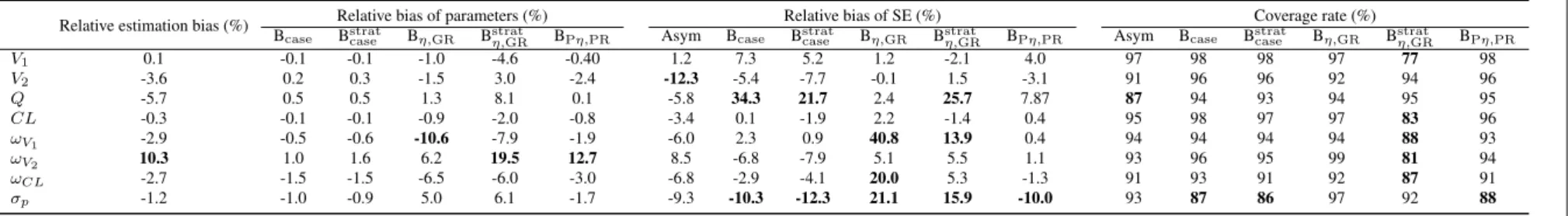
Table 2: Relative estimation bias, relative bootstrap bias, relative bias of standard error (SE) estimates and coverage rate obtained by the asymptotic method (Asym) via the MFand the three bootstrap methods for the unbalanced design with first-order elimination
Relative estimation bias (%) Relative bias of parameters (%) Relative bias of SE (%) Coverage rate (%)
Bcase Bstratcase Bη,GR Bη,GRstrat BPη,PR Asym Bcase Bstratcase Bη,GR Bstratη,GR BPη,PR Asym Bcase Bstratcase Bη,GR Bstratη,GR BPη,PR
V1 0.1 -0.1 -0.1 -1.0 -4.6 -0.40 1.2 7.3 5.2 1.2 -2.1 4.0 97 98 98 97 77 98 V2 -3.6 0.2 0.3 -1.5 3.0 -2.4 -12.3 -5.4 -7.7 -0.1 1.5 -3.1 91 96 96 92 94 96 Q -5.7 0.5 0.5 1.3 8.1 0.1 -5.8 34.3 21.7 2.4 25.7 7.87 87 94 93 94 95 95 CL -0.3 -0.1 -0.1 -0.9 -2.0 -0.8 -3.4 0.1 -1.9 2.2 -1.4 0.4 95 98 97 97 83 96 ωV1 -2.9 -0.5 -0.6 -10.6 -7.9 -1.9 -6.0 2.3 0.9 40.8 13.9 0.4 94 94 94 94 88 93 ωV2 10.3 1.0 1.6 6.2 19.5 12.7 8.5 -6.8 -7.9 5.1 5.5 1.1 93 96 95 99 81 94 ωCL -2.7 -1.5 -1.5 -6.5 -6.0 -3.0 -6.8 -2.9 -4.1 20.0 5.3 -1.3 91 93 91 92 87 91 σp -1.2 -1.0 -0.9 5.0 6.1 -1.7 -9.3 -10.3 -12.3 21.1 15.9 -10.0 93 87 86 97 92 88 Relative bias> 10% and < -10% and coverage < 0.9 are typeset in bold font
Table 3: Parameter estimates and their relative standard errors (RSE) obtained by the asymptotic method (Asym) via the MFand the
bootstrap methods (B=999 samples) for the real dataset
Median of parameter estimates (RSE*(%))
Asym Bcase Bstratcase Bη,GR Bstratη,GR BPη,PR
V1(l) 3.62 (1.9) 3.69 (2.2) 3.69 (2.1) 3.74 (2.1) 3.76 (2.0) 3.71 (2.0) V2(l) 2.90 (5.3) 2.89 (6.4) 2.90 (6.0) 2.96 (6.0) 2.82 (5.9) 2.88 (6.2) Q(l/h) 0.14 (14.9) 0.10 (18.0) 0.10 (16.7) 0.10 (23.1) 0.08 (18.0) 0.13 (15.9) CL(l/h) 0.04 (2.3) 0.04 (2.6) 0.04 (2.6) 0.04 (2.6) 0.04 (2.7) 0.04 (2.5) ωV1(%) 20 +(9.6) 21 (8.7) 21 (8.3) 17 (11.6) 16 (10.3) 19 (9.8) ωQ(%) 111 (12.5) 110 (13.3) 110 (13.5) 95 (22.4) 99 (16.0) 100 (9.6) ωCL(%) 29 (4.9) 29 (6.8) 29 (6.6) 30 (10.5) 29 (14.3) 29 (5.4) ρCL,Q 0.90 (8.2) 0.87 (8.1) 0.86 (7.9) 0.84 (12.1) 0.88 (7.1) 0.94 (5.9) σp(%) 25 (3.8) 24 (6.2) 24 (5.8) 29 (6.7) 29 (7.4) 26 (3.5)
*RSE=SE/asymptotic parameter estimates*100
+The values forω are presented in %, by multiplying the value in SD scale with 100, for example
7 FIGURES
First−order frequent balanced
First−order sparse balanced
0 100 200 300 400 500 Time (h) CONC (µg/ml) 0.01 0.1 1 10 1000 0 100 200 300 400 500 Time (h) CONC (µg/ml) 0.01 0.1 1 10 1000
Mixed−order frequent balanced
First−order frequent unbalanced
0 100 200 300 400 500 Time (h) CONC (µg/ml) 0.01 0.1 1 10 1000 0 100 200 300 400 500 Time (h) CONC (µg/ml) 0.01 0.1 1 10 1000
Fig. 1: Spaghetti plot of examples of simulated data for 4 studied designs: first-order frequent sampling balanced design (N = 30/n = 9) (top left), first-order sparse sampling balanced design (N = 70/n = 4) (top right), mixed-order frequent sampling design (N = 30/n = 9) (bottom left) and first-order frequent sampling unbalanced design (N1= 15/n1= 9; N2= 75/n2= 2) (bottom
First−order frequent sampling −30 −10 0 10 20 30 Rbias of par ameters (%) V1 V2 Q CLωV1ωQωCL ρ σp Rbias of SE (%) V1 V2 Q CLωV1ωQωCL ρ σp −90 −20 0 20 100 120 Co v er age r ate (%) V1 V2 Q CLωV1ωQωCL ρ σp 10 20 70 80 90 100
First−order sparse sampling
−30 −10 0 10 20 30 Rbias of par ameters (%) V1 V2 Q CL ωV1 ωV2ωCL σp Rbias of SE (%) V1 V2 Q CL ωV1 ωV2ωCL σp −90 −20 0 20 100 120 Co v er age r ate (%) V1 V2 Q CL ωV1ωV2ωCL σp 10 20 70 80 90 100
Mixed−order frequent sampling
−30 −10 0 10 20 30 Rbias of par ameters (%) V1 V2 Q VmaxKmωV1ωV2ωVmaxσp Rbias of SE (%) V1 V2 Q VmaxKmωV1ωV2ωVmaxσp −90 −20 0 20 100 120 Co v er age r ate (%) V1 V2 Q VmaxKmωV1ωV2ωVmaxσp 10 20 70 80 90 100 Asym Bcase Bη,GR BPη,PR
Fig. 2: Relative bias of parameter estimates (relative estimation bias and relative bootstrap bias) (left) , relative bias of standard error (SE) estimates (middle) and coverage rate of 95% CI (right), for the asymptotic method (Asym) and the bootstrap methods in the three balanced designs: first-order frequent sampling design (N = 30/n = 9) (top), first-order sparse sampling design (N = 70/n = 4) (middle), mixed-order frequent sampling design (N = 30/n = 9) (bottom).
First−order frequent sampling −100 −50 0 50 100 150 V1V2Q CLωV1ωQωCLρ σp Asym Relativ e error of SE (%) −100 −50 0 50 100 150 V1V2Q CLωV1ωQωCLρ σp Bcase −100 −50 0 50 100 150 V1V2Q CLωV1ωQωCLρ σp Bη,GR −100 −50 0 50 100 150 V1V2Q CLωV1ωQωCLρ σp BPη,PR
First−order sparse sampling
−100 −50 0 50 100 150 V1V2CLωV1ωV2ωCLσp Q −400 −200 0 200 400 600 Asym Relativ e error of SE (%) −100 −50 0 50 100 150 V1V2CLωV1ωV2ωCLσpQ −400 −200 0 200 400 600 Bcase Relativ e error of SE (%) −100 −50 0 50 100 150 V1V2CLωV1ωV2ωCLσpQ −400 −200 0 200 400 600 Bη,GR −100 −50 0 50 100 150 V1V2CLωV1ωV2ωCLσpQ −400 −200 0 200 400 600 BPη,PR
Mixed−order frequent sampling
−100 −50 0 50 100 150 V1V2Q VmaxKmωV1ωV2ωVmσp Asym Relativ e error of SE (%) −100 −50 0 50 100 150 V1V2Q VmaxKmωV1ωV2ωVmaxσp Bcase −100 −50 0 50 100 150 V1V2Q VmaxKmωV1ωV2ωVmaxσp Bη,GR −100 −50 0 50 100 150 V1V2Q VmaxKmωV1ωV2ωVmaxσp BPη,PR
Fig. 3: Boxplot of relative error of standard error (SE) estimates obtained by the asymptotic method (Asym) and the bootstrap methods in the three studied balanced designs: first-order frequent sampling design (N = 30/n = 9) (top), first-order sparse sampling design (N = 70/n = 4) (middle), mixed-order frequent sampling design (N = 30/n = 9) (bottom)
−30 −20 −10 0 10 20 30 40 Rbias of par ameters (%) V1 V2 Q CLωV1ωV2ωCL σp −30 −20 −10 0 10 20 30 40 Rbias of SE (%) V1 V2 Q CLωV1ωV2ωCLσp 70 75 80 85 90 95 100 Co v er age r ate (%) V1 V2 Q CLωV1ωV2ωCL σp Asym Bcase Bcasestrat Bη,GR Bηstrat,GR BPη,PR
Fig. 4: Relative bias of parameter estimates (relative estimation bias and relative bootstrap bias) (left), relative bias of standard error (SE) estimates (middle) and coverage rate of 95% CI (right), for the asymptotic method (Asym) and the bootstrap methods in the unbalanced design (N1= 15/n1= 9; N2= 75/n2= 2) with first-order elimination
−100 0 100 200 300 V1 V2 Q CLωV1ωV2ωCLσp
Asym
Relativ e error of SE (%) −100 0 100 200 300 V1 V2 Q CLωV1ωV2ωCL σpB
case −100 0 100 200 300 V1 V2 Q CLωV1ωV2ωCLσpB
casestrat −100 0 100 200 300 V1 V2 Q CLωV1ωV2ωCLσpB
η,GR Relativ e error of SE (%) −100 0 100 200 300 V1 V2 Q CLωV1ωV2ωCLσpB
ηstrat,GR −100 0 100 200 300 V1 V2 Q CLωV1ωV2ωCLσpB
Pη,PRFig. 5: Boxplot of relative error of standard error (SE) estimates obtained by the asymptotic method (Asym) and the bootstrap methods in the unbalanced design (N1= 15/n1= 9; N2= 75/n2= 2) with first-order elimination
3.2 3.4 3.6 3.8 4.0 V1 ( l )
Asym Bcase Bcasestrat Bη,GR Bη,GR strat BPη,PR 2.4 2.6 2.8 3.0 3.2 3.4 V2 ( l )
Asym Bcase Bcasestrat Bη,GR Bη,GR strat BPη,PR 0.05 0.10 0.15 0.20 Q (l/h)
Asym Bcase Bcasestrat Bη,GR Bη,GR strat BPη,PR 0.036 0.038 0.040 0.042 0.044 CL (l/h)
Asym Bcase Bcasestrat Bη,GR Bη,GR strat BPη,PR 0.10 0.15 0.20 0.25 0.30 ωV 1
Asym Bcase Bcasestrat Bη,GR Bη,GR strat BPη,PR 0.6 0.8 1.0 1.2 1.4 1.6 ωQ
Asym Bcase Bcasestrat Bη,GR Bη,GR strat BPη,PR 0.20 0.25 0.30 0.35 0.40 ωC L
Asym Bcase Bcasestrat Bη,GR Bη,GR strat BPη,PR 0.6 0.8 1.0 1.2 1.4 ρ
Asym Bcase Bcasestrat Bη,GR Bη,GR strat BPη,PR 0.15 0.20 0.25 0.30 0.35 σp
Asym Bcase Bcasestrat Bη,GR Bη,GR strat
BPη,PR
Fig. 6: Plot of median values and 95% confidence intervals of parameter estimates obtained by the asymptotic method (Asym) and the bootstrap methods (B=999 samples) for all parameters of the real dataset. The broken line in each plot represents the value of the parameter estimate obtained with the real dataset. The bootstrap confidence intervals are shown as lines in the plots.
APPENDIX
Appendix A: Transformations of random effects using Eigen Value Decomposition (EVD)
LetS and ˆΩ denote respectively the square symmetric empirical and estimated variance covariance
matri-ces. Let ˆU denote the matrix of rescaled raw estimated random effects (by centrering to ensure to have zero
mean) with the column entries corresponding to the random effects of each parameter. The empirical matrix
S of ˆU is then defined as:
S = Uˆ
TUˆ
N − 1 (A.1)
whereN is the number of subjects
The transformed matrix of random effects ˆU′is defined using the correction matrixAη:
ˆ
U′ = ˆU A
η (A.2)
The matrixAηis formed using the Eigen Value Decomposition (EVD) of the matrixS and the matrix ˆΩ.
Since any square symmetric matrixM can be decomposed by EVD in an expression involving a diagonal
matrix (D) containing the eigenvalues of M in diagonal entries and a orthogonal matrix (V ) (V VT = I, I
is identity matrix) as follows:M = V DVT, we can write the EVD decomposition ofS and ˆΩ as:
S = VSDSVST (A.3)
ˆ
Ω = VΩˆDΩˆVΩˆT (A.4)
whereVΩˆandVS are respectively the orthogonal matrices of ˆΩ and S; DΩˆ andDSare respectively the
diagonal matrices of ˆΩ and S, where theirs diagonal entries are respectively the eigenvalues of ˆΩ and S.
We propose the following solution ofA which makes the variance covariance matrix of the transformed
matrix of random effects ˆU′equal to ˆΩ:
Aη = VSDS−1/2DΩˆ 1/2V ˆ Ω T (A.5) whereDΩˆ 1/2
andDS−1/2 are respectively the diagonal matrices where theirs diagonal entries are
respectively the root square of eigenvalues of ˆΩ and the inverse of root square of eigenvalues of S.
The transposed form of A is:
AηT = VΩˆDΩ1/2ˆ DS−1/2VST (A.6)
Indeed, the variance covariance matrix of ˆU′is equal to ˆΩ, based on the following development:
ˆ U′TUˆ′ N − 1 = ( ˆU Aη)TU Aˆ η N − 1 = AT ηUˆTU Aˆ η N − 1 = A T ηSAη = VΩˆD1/2Ωˆ DS−1/2VSTVSDSVSTVSDS−1/2DΩˆ1/2VΩˆT = VΩˆD 1/2 ˆ Ω [DS −1/2(V STVS)DS(VSTVS)DS−1/2]DΩˆ 1/2V ˆ Ω T = VΩˆD 1/2 ˆ Ω [DS −1/2D SDS−1/2]DΩˆ 1/2V ˆ Ω T = VΩˆD1/2Ωˆ DΩˆ1/2VΩˆT = VΩˆDΩˆVΩˆT = ˆΩ (A.7)
In caseDS−1/2is not invertible (singular) due to some eigenvalues ofDS are close to zero, a
pseudo-inverse matrix is used by inverting only the positive eigenvalues greater than a tolerance of10−6and setting
those lower to zero.
In balanced designs, the transformation of random effects was carried out in the following steps:
1. Center the raw estimated random effects:η˜i= ˆηi− ¯η
2. Calculate the correction matrixAη. Let ˆΩ be the model estimated variance-covariance matrix of
ran-dom effects andS denote the empirical variance-covariance matrix of the centered random effects. The
correction matrix is formed using EVD of these two matrices:Aη= VSDS−1/2DΩˆ
1/2V
ˆ Ω T
3. Transform the centered random effects using the ratioAη:ηˆ
′
i = ˜ηiAη
In unbalanced designs, for example with two groups containing rich and sparse data, the transformation of random effects was carried out in the following steps:
1. Center the raw estimated random effects:η˜i = ˆηi− ¯η and divide them into two groups ˜ηG1 andη˜G2
presenting the centered random effects in group 1 (G1) and group 2 (G2).
2. Calculate the correction matricesAη;G1 andAη;G2. Let ˆΩ be the model estimated variance-covariance
matrix of random effects,S1andS2denote the empirical variance-covariance matrix of the centered
random effectsη˜G1 andη˜G2 respectively. The correction matrices Aη;G1 andAη;G2 using EVD are
formed as follows: Aη;G1 = VS1DS1 −1/2D ˆ Ω 1/2V ˆ Ω T Aη;G2 = VS2DS2−1/2DΩˆ 1/2V ˆ Ω T
whereVS1andVS2are respectively the orthogonal matrices ofS1andS2;DS1andDS2are respectively
the diagonal matrices ofS1andS2.
3. Transform the centered random effects in each group: ˆ
η′i;G1= ˜ηi;G1Aη;G1
ˆ
η′i;G2= ˜ηi;G2Aη;G2
Appendix B: Transformations of residuals
In balanced designs, the transformation of residuals was carried out in the following steps:
1. Center the raw estimated standardized residuals:˜ϵij= ˆϵij− ¯ϵ
2. Calculate the correction factorAσ
Aσ= 1/σemp
whereσempis simply the empirical standard deviation of the raw standardized residuals
3. Transform the centered residuals using the ratioAσ:ˆϵ
′
ij = ˜ϵijAσ
In unbalanced designs, for example with two groups containing rich and sparse data, the transformation of residuals was carried out in the following steps:
1. Center the raw estimated standardized residuals:˜ϵij= ˆϵij− ¯ϵ and divide them into two groups ˜ϵG1and
˜ϵG2 presenting the centered residuals in group 1 (G1) and group 2 (G2).
2. Calculate the correction factorsAσ;G1andAσ;G2.
Aσ;G1 = 1 σemp;G1 Aσ;G2 = 1 σemp;G2
whereσemp;G1 andσemp;G2 are respectively the empirical standard deviation of the raw standardized
3. Transform the centered residuals in each group:
ˆ
ϵ′ij;G1 = ˜ϵij;G1Aσ;G1
ˆ
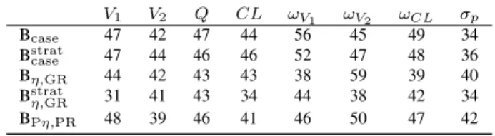
Supplementary tables
Table S1: Coverage rates of 50% CI of parameters in the unbalanced design
V1 V2 Q CL ωV1 ωV2 ωCL σp Bcase 47 42 47 44 56 45 49 34 Bstrat case 47 44 46 46 52 47 48 36 Bη,GR 44 42 43 43 38 59 39 40 Bstratη,GR 31 41 43 34 44 38 42 34 BPη,PR 48 39 46 41 46 50 47 42