Research Article
Giulia Bianco and Elisa Gorla*
Compression for trace zero points on twisted
Edwards curves
DOI: 10.1515/jmc-2015-0039
Received July 27, 2015; revised January 6, 2016; accepted January 14, 2016
Abstract: We propose two optimal representations for the elements of trace zero subgroups of twisted Edwards
curves. For both representations, we provide efficient compression and decompression algorithms. The effi-ciency of the algorithm is compared with the effieffi-ciency of similar algorithms on elliptic curves in Weierstrass form.
Keywords: Trace zero subgroup, Edwards curve, compression, decompression MSC 2010: 14G50, 94A60
||
Communicated by: Alfred Menezes
Introduction
Trace zero subgroups are subgroups of the groups of points of an elliptic curve over extension fields. They were first proposed for use in public key cryptography by Frey in [11]. A main advantage of trace zero sub-groups is that they offer a better scalar multiplication performance than the whole group of points of an elliptic curve of approximately the same cardinality. This allows a fast arithmetic, which can speed up the calculations by 30% compared with elliptic curves groups (see, e.g., [14] for the case of hyperelliptic curves, [3, 8] for elliptic curves over fields of even characteristic). In addition, computing the cardinality of a trace zero subgroup is more efficient than for the group of points of an elliptic curve of approximately the same cardinality. Moreover, even if the trace zero subgroup is a proper subgroup of the group of rational points of the curve over an extension field, the Discrete Logarithm Problem (DLP) in the two groups has the same complexity. Hence, when working over non-prime fields, we may restrict to the trace zero subgroup to gain a more efficient arithmetic without compromising the security. Finally, in the context of pairings trace zero subgroups of supersingular elliptic curves offer higher security than supersingular elliptic curves of the same bit-size, as shown in [16].
The problem of how to compress the elements of the trace zero subgroup of an elliptic or hyperelliptic curve is the analogue of torus-based cryptography in finite fields. For elliptic and hyperelliptic curves this problem has been studied by many authors, see [12–16, 18].
Edwards curves were first introduced by Edwards in [9] as a normal form for elliptic curves. They were proposed for use in elliptic curve cryptography by Bernstein and Lange in [4]. Twisted Edwards curves were introduced shortly after in [6]. They are relevant from a cryptographic point of view since the group operation can be computed very efficiently and via strongly unified formulas, i.e., formulas that do not distinguish between addition and doubling. This makes them more resistant to side-channel attacks. We refer to [4–6] for a detailed discussion on the advantages of Edwards curves.
Giulia Bianco: Institut de Mathématiques, Université de Neuchâtel, Rue Emile-Argand 11, CH-2000 Neuchâtel, Switzerland,
e-mail: [email protected]
*Corresponding author: Elisa Gorla: Institut de Mathématiques, Université de Neuchâtel, Rue Emile-Argand 11,
In this paper, we provide two efficient representations for the elements of the trace zero subgroups of twisted Edwards curves. The first one follows ideas from [12] and it is based on Weil restriction of scalars and Semaev’s summation polynomials. The second one follows ideas from [13] and it makes use of rational func-tions on the curve. Some obstacles have to be overcome in adapting these ideas to Edwards curves, especially for adapting the method from [13].
Given a twisted Edwards curve defined over a finite field 𝔽qof odd characteristic and a field extension of odd prime degree 𝔽q⊂ 𝔽qn, we consider the trace zero subgroupTnof the group of 𝔽qn-rational points of
the curve. We give two efficiently computable maps fromTnto 𝔽nq−1, such that inverse images can also be efficiently computed. One of our maps identifies Frobenius conjugates, while the other identifies Frobenius conjugates and opposites of points. SinceTn has orderO(qn−1), our maps are optimal representations of Tnmodulo Frobenius equivalence. For both representations we provide efficient algorithms to compute the image and the preimage of an element, that is, to compress and decompress points. We also compare with the corresponding algorithms for trace zero subgroups of elliptic curves in short Weierstrass form.
The article is organized as follows. In Section 1 we give some preliminaries on twisted Edwards curves, finite fields, trace zero subgroups, and representations. In Section 2 we present our first optimal representa-tion based on Weil restricrepresenta-tion and summarepresenta-tions polynomials, and give compression and decompression algo-rithms. We then make explicit computations for the cases n = 3 and n = 5, and compare execution times of our Magma implementation with those of the corresponding algorithms for elliptic curves in short Weierstrass form. In Section 3 we propose another representation based on rational functions, with the corresponding algorithms, computations and efficiency comparison.
1 Preliminaries and notations
Let 𝔽qbe a finite field of odd characteristic and let 𝔽q ⊂ 𝔽qnbe a field extension of odd prime degree. Choose a
normal basis {α, αq, . . . , αqn−1} of 𝔽qnover 𝔽q. If n|q − 1, let 𝔽qn= 𝔽q[ξ ]/(ξn− μ), where μ is not a nth-power
in 𝔽q, and choose the basis {1, ξ, . . . , ξn−1} of 𝔽qnover 𝔽q. Either of these choices is suitable for computation,
since it produces sparse equations. When writing explicit formulas, we always assume that we are in the latter situation.
When counting the number of operations in our computations, we denote respectively by M, S, and I mul-tiplications, squarings, and inversions in the field. We do not take into account additions and multiplications by constants. The timings for the implementation of our algorithms in Magma refer to version V2.20-7 of the software, running on a single 3 GHz core.
1.1 Twisted Edwards curves
Definition 1.1. A twisted Edwards curve over 𝔽qis a plane curve of equation
Ea,d: ax2+ y2= 1 + dx2y2,
where a, d ∈ 𝔽q\ {0} and a ̸= d. An Edwards curve is a twisted Edwards curve with a = 1.
Twisted Edwards curves are curves of geometric genus one with two ordinary multiple points, namely the two points at infinity. Since Ea,dis birationally equivalent to a smooth elliptic curve, one can define a group law on the set of points of Ea,d, called the twisted Edwards addition law.
Definition 1.2. The sum of two points P1= (x1, y1) and P2= (x2, y2) of Ea,dis defined as
P1+ P2= (x1, y1) + (x2, y2) = (
x1y2+ x2y1
1 + dx1x2y1y2
, y1y2− ax1x2 1 − dx1x2y1y2).
We refer to [4, Section 3] and [6, Section 6] for a detailed discussion on the formulas and a proof of correctness. The pointO = (0, 1) ∈ Ea,dis the neutral element of the addition, and we denote by −P the additive inverse
of P. If P = (x, y), then −P = (−x, y). We let O= (0, −1) ∈ Ea,d, and denote by Ω1= [1, 0, 0] and Ω2= [0, 1, 0]
the two points at infinity of Ea,d.
Edwards curves were introduced in [9] as a convenient normal form for elliptic curves. Over an alge-braically closed field, every elliptic curve in Weierstrass form is birationally equivalent to an Edwards curve, and vice versa. This is however not the case over 𝔽q, where Edwards curves represent only a fraction of ellip-tic curves in Weierstrass form. In [6, Theorem 3.2] it is shown that a twisted Edwards curve defined over 𝔽q is birationally equivalent over 𝔽qto an elliptic curve in Montgomery form, and conversely, an elliptic curve in Montgomery form defined over 𝔽qis birationally equivalent over 𝔽qto a twisted Edwards curve.
Proposition 1.3. The twisted Edwards curve Ea,ddefined over 𝔽qis birationally equivalent over 𝔽qto the elliptic
curve in Montgomery form EA,B: By2= x3+ Ax2+ x, where A = 2aa+d−dand B = a4−d. Let Ea,dand EA,Bbe the
projective closures of Ea,dand EA,B, respectively. The birational isomorphism Φ : EA,B→ Ea,dis defined via
ϕ([x, y, z]) ={{
{
[x(x + z), y(x − z), y(x + z)] if [x, y, z] ̸∈ {Ω2, (0, 0)},
[By(x + z), By2− x2− Axz − z2, By2+ x2+ Axz + z2] if [x, y, z] ̸∈ {Q1, Q2, Q3, Q4},
where
Q1= (√d + √a
√d − √a, 0), Q2= (
√d − √a
√d + √a, 0), Q3= (−1, √d), Q4= (−1, −√d) ∈ EA,B.
Proof. It is easy to check that Φ is well defined and Φ(Q1) = Φ(Q2) = Ω1and Φ(Q3) = Φ(Q4) = Ω2. Moreover,
Φ is injective on EA,B\ {Q1, Q2, Q3, Q4}, and its birational inverse is Ψ : Ea,d\ {Ω1, Ω2} → EA,Bgiven by Ψ([x, y, z]) ={{
{
[x(z + y), z(z + y), x(z − y)] if [x, y, z] ̸= O, [z(z + y)(z − y), x(az2− dy2), z(z − y)2] if [x, y, z] ̸= O.
Moreover, the twisted Edwards addition law corresponds to the usual addition law on the birationally isomor-phic elliptic curve in Montgomery form, as shown in [4, Theorem 3.2]. Similarly to elliptic curves in Mont-gomery or Weierstrass form, the twisted Edwards addition law has a geometric interpretation.
Proposition 1.4 ([1, Section 4]). Let P1, P2∈ Ea,d, and let C be the projective conic passing through P1, P2, Ω1,
Ω2, andO. Then, the point P1+ P2is the symmetric with respect to the y-axis of the eighth point of intersection
between Ea,dand C.
1.2 Trace zero subgroups
Let Ea,dbe a twisted Edwards curve defined over 𝔽q. We denote by Ea,d(𝔽qn) the group of 𝔽qn-rational points
of Ea,d, by P∞any point at infinity of Ea,d, and by φ the Frobenius endomorphism on Ea,ddefined as follows:
φ : Ea,d→ Ea,d, (x, y) → (xq, yq), P∞→ P∞.
Definition 1.5. The trace zero subgroupTnof Ea,d(𝔽qn) is the kernel of the trace map
Tr : Ea,d(𝔽qn) → Ea,d(𝔽q), P → P + φ(P) + φ2(P) + ⋅ ⋅ ⋅ + φn−1(P).
We can viewTnas the 𝔽q-rational points of an abelian variety of dimension n − 1 defined over 𝔽q, called the trace zero variety. We refer to [2] for a construction and the basic properties of the trace zero variety. The following result is an easy consequence of [2, Proposition 7.13].
Proposition 1.6. The sequence
0 → Ea,d(𝔽q) → Ea,d(𝔽qn)
φ−id
→ Tn→ 0
1.3 Representations
Definition 1.7. A representation of size ℓ for the elements of a finite set G is a map
R: G → 𝔽ℓ 2.
Notice that, in our setup, a representationR is not necessarily injective. Nevertheless, any representation induces an injective representation
R: G/∼ → 𝔽ℓ2,
where g ∼ h if and only if R(g) = R(h) for any g, h ∈ G.
Definition 1.8. LetA be a family of abelian varieties of fixed dimension d. An optimal representation for A is
a family of representationsR: A(𝔽q) → 𝔽ℓ2for all finite fields 𝔽qand for all A ∈ A defined over 𝔽q, with the property that
ℓ = ℓ(q) = ⌈log2|A(𝔽q)|⌉ + O(1) = d⌈log2q⌉ + O(1).
We also say that eachR is an optimal representation for the elements of A(𝔽q).
Given g ∈ A(𝔽q), x ∈ Im R, we refer to computing R(g) as compression and R−1(x) as decompression. Intuitively, a representation is optimal if ℓ(q) is the smallest possible length of a binary representation of the elements of A(𝔽q), up to an additive constant. In particular, the length of a representation is regarded as a function of q, while the dimension d of the varieties is assumed to be constant. Notice moreover that, if |R−1(x)| ∈ O(1) as a function of q, then
ℓ(q) = ⌈log2|A(𝔽q)|⌉ = ⌈log2|A(𝔽q)/∼|⌉ + O(1).
In particular, optimality of a representation does not depend on the number of elements that are identified, under the assumption that this number is upper bounded by a constant in q. Therefore, Definition 1.8 is well-posed.
Remark 1.9. The problem of representing the elements of 𝔽qvia binary strings of length ⌈log2q⌉ is well
stud-ied. Therefore, an optimal representation forA may be given via a family of maps R: A(𝔽q) → 𝔽dq× 𝔽k2,
where k ∈ O(1).
The problem of finding an optimal representation has been studied for the following families of abelian vari-eties: elliptic curves, Jacobians of hyperelliptic curves of fixed genus, trace zero varieties of elliptic or hyperel-liptic curves of fixed genus and with respect to a field extension of fixed degree. One may also letA consist of only one element, e.g., the multiplicative group or its primitive subgroup. Finding an optimal representation for the latter is at the core of torus-based cryptography.
In this paper, we letA be the set of trace zero varieties of Edwards curves with respect to a field extension of fixed degree n. We construct two optimal representations for the elements ofTn, with the property that each element in the image has at most 2n, respectively, n inverse images.
2 An optimal representation using summation polynomials
Let 𝔽qbe a finite field of odd characteristic and let Ea,dbe the twisted Edwards curve of equationax2+ y2= 1 + dx2y2,
where a, d ∈ 𝔽q\ {0} and a ̸= d. Following ideas from [12], in this section we use Weil restriction of scalars and Semaev’s summation polynomials to write an equation for the subgroupTn. Similarly to the case of elliptic curves in Weierstrass form, a point P = (x, y) ∈ Ea,d(𝔽qn) can be represented via y ∈ 𝔽qn. Using the
pair of points ±P ∈ Ea,d(𝔽qn) can be represented by the element (y0, . . . , yn−1) ∈ 𝔽nqcorresponding to y ∈ 𝔽qn
under the isomorphism 𝔽qn ≅ 𝔽nqinduced by the chosen basis. Having an equation forTnallows us to drop one
of the yi’s and represent each pair ±P via n − 1 coordinates in 𝔽q, thus providing an optimal representation for the elements ofTn. In order to make computation of the compression and decompression maps more efficient, we modify this basic idea and use the elementary symmetric functions of y, yq, . . . , yqn−1instead of the vector (y0, . . . , yn−1) ∈ 𝔽nq.
Summation polynomials were introduced by Semaev in [17] for elliptic curves in Weierstrass form. Here we use them in the form for Edwards curves from [10].
Definition 2.1. The n-th summation polynomial is denoted by fnand defined recursively by
f3(z1, z2, z3) = (z21z22− z21− z22+ ad−1)z32+ 2(d − a)d−1z1z2z3+ ad−1(z21+ z22− 1) − z21z22,
fn(z1, . . . , zn) = rest(fn−k(z1, . . . , zn−k−1, t), fk+2(zn−k, . . . , zn, t))
for all n ≥ 4 and for all 1 ≤ k ≤ n − 3, where rest(fi, fj) denotes the resultant of fiand fjwith respect to t. The next theorem summarizes the properties of summation polynomials.
Theorem 2.2 ([17, Section 2] and [10, Section 2.3.1]). Let fn∈ 𝔽q[z1, . . . , zn], n ≥ 3, be the n-th summation
polynomial. Denote by 𝔽q⊂ k a field extension, and by k its algebraic closure. Then, the following hold: (i) fnis absolutely irreducible, symmetric, and has degree 2n−2in each of the variables.
(ii) (β1, . . . , βn) ∈ knis a root of fnif and only if there exist α1, . . . , αn∈ k such that Pi= (αi, βi) ∈ Ea,d(k) and
P1+ ⋅ ⋅ ⋅ + Pn= O.
By the previous theorem, if P = (x, y) ∈ Tn, then
fn(y, yq, . . . , yq
n−1
) = 0. (2.1)
A partial converse and exceptions to the opposite implication are given in the next proposition.
Proposition 2.3 ([12, Lemma 1 and Proposition 4]). Let Ea,d be a twisted Edwards curve and denote by
Ea,d[m] its m-torsion points. Then, we have the following: (1) T3= {(x, y) ∈ Ea,d(𝔽q3) | f3(y, yq, yq
2 ) = 0},
(2) T5∪ Ea,d[3](𝔽q) = {(x, y) ∈ Ea,d(𝔽q5) | f5(y, yq, . . . , yq 4
) = 0}, (3) Tn∪ ⋃⌊
n 2⌋
k=1Ea,d[n − 2k](𝔽q) ⊆ {(x, y) ∈ Ea,d(𝔽qn) | fn(y, y
q, . . . , yqn−1
) = 0} for n ≥ 7.
Proof. The proof proceeds as in [12, Lemma 1 and Proposition 4], after observing that for any odd prime n
one has Ea,d[2] ∩ Tn= {O}.
Remark 2.4. Proposition 2.3 raises the question of efficiently deciding, for each root y ∈ 𝔽qnof equation (2.1),
whether the corresponding points (±x, y) ∈ Ea,dare elements ofTn. However, this issue is easily solved in the two cases of major interest n = 3 and n = 5. In fact, we have the following:
∙ By Proposition 2.3 (1), (±x, y) ∈ T3if and only if x ∈ 𝔽q3.
∙ By Proposition 2.3 (2), (±x, y) ∈ T5if and only if x ∈ 𝔽q5 and (±x, y) ̸∈ Ea,d[3](𝔽q) \ {O}. By storing the listL of the y-coordinates of the elements of Ea,d[3](𝔽q) \ {O}, one can easily decide whether a point of
Ea,d(𝔽q5) of coordinates (x, y) belongs to T5by checking that y ̸∈ L. Notice that L consists of at most 4 elements of 𝔽q.
Using the above considerations as a starting point, we can give an optimal representation for the points ofTn with efficient compression and decompression algorithms.
Step 1. Denote by e1, . . . , enthe elementary symmetric functions in n variables. Represent (x, y) ∈ Tnvia
n − 1 of the elementary symmetric functions evaluated at y, yq, . . . , yqn−1
. We obtain an efficiently computable optimal representation
R: Tn→ 𝔽nq−1, (x, y) → (ei(y, yq, . . . , yq
n−1
Algorithm 1.Compression
Input: P = (x, y) ∈ Tn
Output:R(P) ∈ 𝔽nq−1
1: Write y = y0α + ⋅ ⋅ ⋅ + yn−1αqn−1.
2: Compute ei= ̃ei(y0, . . . , yn−1) for i = 1, . . . , n − 1.
3: return (e1, . . . , en−1)
Step 2. Since the polynomial fn(z1, . . . , zn) is symmetric, we can write it uniquely as a polynomial
gn(e1, . . . , en) ∈ 𝔽q[e1, . . . , en]. Therefore, the equation
gn(e1, . . . , en) = 0
describes trace zero points (with the exceptions seen in Proposition 2.3) via the equations
e1= ̃e1(y0, . . . , yn−1), . . . , en= ̃en(y0, . . . , yn−1), (2.3) where the polynomials ̃e1, . . . , ̃enare obtained from the polynomials
e1(y, yq, . . . , yq
n−1
), . . . , en(y, yq, . . . , yq
n−1 )
by Weil restriction of scalars with respect to the chosen basis of 𝔽qn over 𝔽q, and reducing modulo yq
i − yi for i ∈ {0, . . . , n − 1}. Notice that the reduction simplifies the equations by drastically reducing their degrees. Moreover, it does not alter their values when evaluated over 𝔽q.
Step 3. For (e1, . . . , en−1) ∈ R(Tn), we first solve
gn(e1, . . . , en−1, t) = 0
for t. For any solution en∈ 𝔽q, we solve system (2.3) to find (y0, . . . , yn−1) ∈ 𝔽nq, corresponding to y ∈ 𝔽qn.
From y we can recover x in the usual way (see also Remark 2.4).
Notice that gn(e1, . . . , en, ) is not linear in any of the variables for n ≥ 3, hence in step 3 we may find more than one value for en. This corresponds to the fact thatR may identify more than just opposites and Frobenius conjugates. However, this is a rare phenomenon, and for a generic point P ∈ Tn,R−1(R(P)) consists only of ±P and their Frobenius conjugates. We come back to this discussion in Section 2.2, where we discuss this issue for n = 5.
The pseudocode of a compression and a decompression algorithm for the elements ofTnare given in Algorithms 1 and 2, respectively.
2.1 Explicit equations, complexity, and timings for
n = 3
In this subsection we give explicit equations for trace zero point compression and decompression on twisted Edwards curves for n = 3. We also estimate the number of operations needed for the computations, present some timings obtained with Magma, and compare with the results from [12] for elliptic curves in short Weier-strass form.
The symmetrized third summation polynomial for Ea,dis
g3(e1, e2, e3) = e21− 1 + (d/a)(e32− e22) + (2d/a)e1e3− 2e2+ ((−2a + 2d)/a)e3, (2.4)
where e1, e2and e3are the elementary symmetric polynomials in y, yq, yq
2 , i.e., { { { { { { { { { e1= y + yq+ yq 2 , e2= y1+q+ y1+q 2 + yq+q2, e3= y1+q+q 2 . (2.5)
Algorithm 2.Decompression Input: (e1, . . . , en−1) ∈ 𝔽nq−1 Output:R−1(e1, . . . , en−1) ⊆ Tn 1: Solve gn(e1, . . . , en−1, t) = 0 for t in 𝔽q. 2: T ← list of solutions of gn(e1, . . . , en−1, t) = 0 in 𝔽q. 3: foren∈ T do
4: Find a solution in 𝔽nqof the system { { { { { { { { { e1= ̃e1(y0, . . . , yn−1), .. . en= ̃en(y0, . . . , yn−1), if it exists.
5: Any time a solution (y0, . . . , yn−1) is found, compute y = y0α + ⋅ ⋅ ⋅ + yn−1αq
n−1 .
6: Recover one of the corresponding x-coordinates using the curve equation.
7: end for
8: if (x, y) ∈ Tnthen
9: add P = (±x, y) and all its Frobenius conjugates to the list L of output points. 10: end if
11: return L
The symmetrized third summation polynomial for an elliptic curve in short Weierstrass form is
G3(e1, e2, e3) = e22− 4e1e3− 4Be1− 2Ae2+ A2. (2.6)
Notice that, while G3is linear in e1and e3, g3is of degree 2 in each variable. In particular, none of e1, e2, e3is
determined uniquely by the other two as is the case of elliptic curves in Weierstrass form. However, applying the change of coordinates
{ { { { { { { t1= e1, t2= e3+ e2, t3= e3− e2, (2.7)
to g3, we obtain the polynomial
̃g3(t1, t2, t3) = t21+ (d/a)(t2t3+ t1t2+ t1t3) + ((d/a) − 2)t2+ dt3− 1, (2.8)
that is linear in both t2and t3.
Applying Weil restriction of scalars to the combination of (2.5) and (2.7) (and following the conventions of Section 1), we obtain { { { { { { { t1= 3y0,
t2= y30− 3μy0y1y2+ μy13+ μ2y32+ 3y20− 3μy1y2,
t3= y30− 3μy0y1y2+ μy13+ μ2y32− 3y20+ 3μy1y2,
(2.9)
which expresses t1, t2, t3as polynomials in y0, y1, y2.
Point compression. For compression of a point P = (x, y) ∈ T3, we use the first two coordinates from (2.7)
and (2.9), obtaining
R(P) = (t1, t2) = (3y0, y30− 3μy0y1y2+ μy31+ μ2y32+ 3y20− 3μy1y2).
If we compute t2as (y0+ 1)(y20− 3μy1y2) + μy31+ μ2y 3
2+ 2y20, the cost of computingR(P) is 3S+4M in 𝔽q. In the case of elliptic curves in short Weierstrass form, computing the representation of a point is less expen-sive, as it takes 1S+1M in 𝔽qor 1M in 𝔽qwith the two methods presented in [12, Section 5].
Point decompression. In order to decompress (t1, t2) ∈ Im R we proceed as follows.
Step 1. Given (t1, t2) ∈ Im R, solve ̃g3(t1, t2, t3) = 0 for t3. If t1+ t2+ a = 0, then ̃g3(t1, t2, t3) = 0 for all
t3∈ 𝔽q. If t1+ t2+ a ̸= 0, then
t3= −((d/a) − 2)t2+ (d/a)t1
t2+ (t1+ 1)(t1− 1)
(d/a)(t1+ t2+ a)
. Hence, t3can be computed with 3M+1I in 𝔽q.
Step 2. Given (t1, t2, t3), we solve system (2.9) for y0, y1, y2. Notice that, since the tiare obtained from the eiby a linear change of coordinates, all considerations from [12] apply to our situation. In particular, one can compute y from (t1, t2, t3) with at most 3S+3M+1I, 1 square root and 2 cube roots in 𝔽q.
Summarizing, the complete decompression algorithm takes at most 3S+6M+2I, 1 square root, and 2 cube roots in 𝔽q. For elliptic curves in short Weierstrass form, decompression takes at most 3S+5M+2I, 1 square root and 2 cube roots in 𝔽qor 4S+4M+2I, 1 square roots and 2 cube roots in 𝔽q, depending on the method used. We refer the interested reader to [12, Section 5] for details on the complexity of the computation for curves in short Weierstrass form.
Remark 2.5. Notice that one can also use (t1, t3) as an optimal representation of (x, y) ∈ T3, and then solve
̃g3for t2in order to recover y. This choice is analogous to the one we have made, and the computational cost
of compression and decompression does not change.
Remark 2.6. The symmetry of twisted Edwards curves makes the computation of point addition on these
curves more efficient than on elliptic curves in short Weierstrass form. However, the same symmetry results in summation polynomials of higher degree and with a denser support. This explains our empirical obser-vation that the summation polynomials in the elementary symmetric functions for elliptic curves in short Weierstrass form are sparser than those for twisted Edwards curves for n = 3, 5, even though for both curves they have the same degree 2n−2. For n = 3, this behavior is apparent if one compares equations (2.4) and (2.6). Therefore, one should expect that compression and decompression for a representation based on sum-mation polynomials for twisted Edwards curves are less efficient than for elliptic curves in short Weierstrass form. This is confirmed by our findings.
The following examples and statistics have been implemented in Magma [7].
Example 2.7. Let q = 279− 67 and μ = 3. We choose the following random curves, defined and birationally equivalent over 𝔽q:
Ea,d: 31468753957068040687814x2+ y2= 1 + 192697821276638966498997x2y2 and
E : y2= x3+ 292467848427659499478503x + 361361026736404004345421.
We choose a random point of trace zero P∈ E(𝔽q3), and let P be the corresponding point on Ea,d. For brevity, here we only write the x-coordinates of points of E and the y-coordinates of points of Ea,d:
P= 346560928146076959314753ξ2+ 456826539628535981034212ξ
+ 344167470403026652826672,
P = 208520713897518236215966ξ2+ 451121944550219947368811ξ
+ 68041089860429901306252.
We represent the points of E using the compression coordinates (t1, t2) from [12, Section 5]. Denote by R and
Rthe representation maps on E
a,dand E, respectively. We compute
R(P) = (344167470403026652826672, 334324534997495805088214), R(P) = (204123269581289703918756, 98788782936076524413527).
Bit-length of |T3| 192 224 256
Compression on E 0.006 0.005 0.006 Compression on Ea,d 0.016 0.017 0.015
Decompression on E 0.81 2.40 1.20 Decompression on Ea,d 0.88 2.44 1.17
Table 1. Average times for compression and decompression
on elliptic curves in short Weierstrass form and twisted Edwards curves.
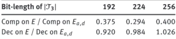
Bit-length of |T3| 192 224 256
Comp on E / Comp on Ea,d 0.375 0.294 0.400
Dec on E / Dec on Ea,d 0.920 0.984 1.026
Table 2. Ratios between the average times for point
compression and decompression on elliptic curves in short Weierstrass form and twisted Edwards curves.
We now apply the corresponding decompression algorithms toR(P) and R(P). We obtain R−1(344167470403026652826672, 334324534997495805088214) = {346560928146076959314753ξ2+ 456826539628535981034212ξ + 344167470403026652826672, 164759498614507503187493ξ2+ 361520690988197751534381ξ + 344167470403026652826672, 93142483046730124850775ξ2+ 390578588997895442137449ξ + 344167470403026652826672},
which are exactly the x-coordinate of Pand its Frobenius conjugates. Similarly,
R−1(204123269581289703918756, 98788782936076524413527) = {208520713897518236215966ξ2+ 451121944550219947368811ξ + 68041089860429901306252, 539321536961066855011167ξ2+ 237431391097642968386719ξ + 68041089860429901306252, 461083568756044083478909ξ2+ 520372483966766258950512ξ + 68041089860429901306252},
which are exactly the y-coordinate of P and its Frobenius conjugates.
We now give an estimate of the average time of compression and decompression for groups of different bit-size. We consider primes q1, q2and q3such that 3|qi− 1 for all i, of bit-length 96, 112 and 128, respectively. For each qi, we consider five pairs of birationally equivalent curves (E, Ea,d), defined over 𝔽qi, such that
the order ofT3is prime of bit-length respectively 192, 224 and 256. On each pair of curves we randomly
choose 20000 pairs of points (P, P) of trace zero, as in Example 2.7. For each pair of points, we compute R(P), R(P), R−1(R(P)), R−1(R(P)). For each computation, we consider the average time in milliseconds
for each curve, and then the averages over the five curves. The average computation times are reported in Table 1.
Table 2 contains the ratios between the average times for point compression and decompression on el-liptic curves in short Weierstrass form and twisted Edwards curves.
2.2 Explicit equations, complexity, and timings for
n = 5
In this subsection we treat in detail the case n = 5. We compute explicit equations for compression and de-compression, give an estimate of the complexity of the computations in terms of the number of operations, and give some timings computed in Magma. We also compare the results with those obtained in [12] for el-liptic curves in short Weierstrass form.
The fifth Semaev polynomial f5 for a twisted Edwards curve has degree 40, while for curves in short
Weierstrass form it has degree 32. The first polynomial also contains many more terms than the second. This agrees with what we observed in Remark 2.6 for the case n = 3. The symmetrized fifth summation polyno-mial g5has degree 8 for both Weierstrass and Edwards curves. However, for Edwards curves g5has degree 8
in each variable, while for elliptic curves in short Weierstrass form it has degree 6 in some of the variables. Because of these reasons, we expect that compression and decompression for a trace zero subgroup coming from a twisted Edwards curve are less efficient than for one coming from a curve in short Weierstrass form.
For fields such that 16|q − 1, we perform a linear change of coordinates on the eiin order to obtain a polynomial ̃g5, of degree strictly less than 8 in some variable. The polynomial g5is too big to be printed here.
However, denoting by (g5)8the part of g5which is homogeneous of degree 8, we have that
(g5)8(e1, . . . , e5) = e81+ (d/a)4(e82+ e83) + (d/a)8(e84+ e85). (2.10)
Let μ1∈ 𝔽qbe a primitive 16-th roots of unity. Then, we can factor t8+ s8over 𝔽qas
t8+ s8= (t − μ1s)(t + μ1s)r6(t, s).
Therefore, (2.10) can be written in the form
(g5)8= e81+ (d/a)4(e2− μ1e3)(e2+ μ1e3)r6(e2, e3) + (d/a)8(e84+ e85).
Hence, after performing the change of coordinates { { { { { { { t2= e2− μ1e3, t3= e2+ μ1e3, ti= ei for i = 1, 4, 5,
we obtain a polynomial ̃g5(t1, . . . , t5) of degree 8 in t1, t4, t5, and degree 7 in t2, t3.
Example 2.8. Let q = 210− 3, μ = 2. Consider the Edwards curve E
1,486of equation x2+ y2= 1 + 6x2y2. Let
P ∈ T5be the point
P = (u, v) = (951ξ4+ 338ξ3+ 246ξ2+ 934ξ + 133, 650ξ4+ 927ξ3+ 301ξ2+ 171ξ + 973).
The compression of P isR(P) = (e1, e2, e3, e4) = (686, 289, 865, 418). In order to decompress, we solve
g5(e1, e2, e3, e4, t) = g5(686, 289, 865, 418, t)
= 71t8+ 705t7+ 1007t6+ 970t5+ 233t4+ 1014t3+ 356t2+ 198t + 575 = 0, which has a unique solution e5= 790 ∈ 𝔽q. In order to recover the value of y up to Frobenius conjugates, we find a root in 𝔽q5of
y5− e1y4+ e2y3− e3y2+ e4y − e5= y5+ 335y4+ 289y3+ 156y2+ 418y + 231.
Notice that the five roots are Frobenius conjugates of each other. From one y ∈ 𝔽q5 we can recompute x via the curve equation, hence recover one of the Frobenius conjugates of ±P. So the decompression algorithm returnsR−1(R(P)) = {±P, ±φ(P), ±φ2
(P), ±φ3(P), ±φ4(P)}.
We now give an example that presents some indeterminacy in the decompression algorithm.
Example 2.9. Let q = 210− 3 and consider the Edwards curve
E210,924: 210x2+ y2= 1 + 924x2y2
and the point
Bit-length of |T5| 192 224 256
Compression on E 0.057 0.055 0.060 Compression on Ea,d 0.049 0.058 0.053
Decompression on E 64.17 104.31 121.51 Decompression on Ea,d 63.66 104.45 121.42
Table 3. Average times for compression and decompression
on elliptic curves in short Weierstrass form and twisted Edwards curves.
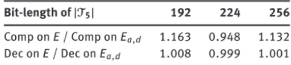
Bit-length of |T5| 192 224 256
Comp on E / Comp on Ea,d 1.163 0.948 1.132
Dec on E / Dec on Ea,d 1.008 0.999 1.001
Table 4. Ratios between the average times for point
compression and decompression on elliptic curves in short Weierstrass form and twisted Edwards curves.
The compressed representation of P isR(P) = (e1, e2, e3, e4) = (310, 887, 19, 660). The decompressing
equation is
g5(e1, e2, e3, e4, t) = 62t8+ 502t7+ 388t6+ 294t5+ 2t4+ 466t3+ 723t2+ 55t + 388 = 0,
which has solutions e5= 428, e5= 835, e5 = 550 ∈ 𝔽q. By solving the equation
y5− e1y4+ e2y3− e3y2+ e4y − e5= y5+ 310y4+ 887y3+ 19y2+ 660y + 593 = 0,
we recover the y-coordinate of P and all its Frobenius conjugates. By solving the equation
y5− e1y4+ e2y3− e3y2+ e4y − e5= y5+ 310y4+ 887y3+ 19y2+ 660y + 186 = 0,
we find roots in 𝔽q5, which do not correspond to points of trace zero. By solving the equation y5− e1y4+ e2y3− e3y2+ e4y − e5 = y5+ 310y4+ 887y3+ 19y2+ 660y + 471 = 0,
we find Q ∈ T5which is not a Frobenius conjugate of P. Hence, in this case
R−1(R(P)) = {±P, . . . , ±φ4
(P), ±Q, . . . , ±φ4(Q)}.
Denote byT5/ ∼ the quotient of T5by the equivalence relation that identifies opposite points and Frobenius
conjugates. The representation (2.2) induces a representation R:T
5/ ∼ → 𝔽4q.
In the previous example we showed thatRis not injective. Nevertheless, an easy heuristic argument shows that a generic (e1, . . . , e4) ∈ Im Rhas exactly one inverse image. In order to support the heuristics, we tested
15 000 random points in the trace zero subgroupT5of 15 Edwards curves. The groups had prime cardinality
and bit-length 192, 224 and 256. For any random point P we computed the cardinality ofR−1(R(P)), and found that it is 1 for about 91% of the points, 2 for about 8.5% of the points, and 3 for about 0.5% of the points. We also found a few points for which |R−1(R(P))| = 4, but the percentage was less than 0.02%. Finally, we did not find any points for which 4 < |R−1(R(P))| ≤ 8.
In order to test the efficiency of the compression and decompression algorithms for n = 5, we have im-plemented them in Magma [7]. We consider primes q1, q2and q3of bit-length 48, 56 and 64, respectively.
We choose primes such that 5|qi− 1 for all i. For each qiwe consider five pairs of birationally equivalent curves (E, Ea,d) defined over 𝔽qi, such that the order ofT5is prime of bit-length 192, 224 and 256,
respec-tively. Table 3 contains the average times for compression and decompression in milliseconds. Each average is computed on a set of 20 000 randomly chosen points on each of the five curves.
Table 4 contains the ratios between the average times for point compression and decompression on el-liptic curves in short Weierstrass form and twisted Edwards curves.
3 An optimal representation using rational functions
Let Ea,dbe a twisted Edwards curve defined over 𝔽q. In this section, we propose another optimal representa-tion for the trace zero subgroupTn⊂ Ea,d(𝔽qn) using rational functions.
In [13] Gorla and Massierer propose to represent an element P ∈ Tnvia the coefficients of the rational function which corresponds to the principal divisor P + φ(P) + ⋅ ⋅ ⋅ + φn−1(P) − nO on the elliptic curve. Op-timality of the representation depends on the fact that the rational function associated to this divisor has a special form, and can therefore be represented using n − 1 coefficients in 𝔽q. If we consider a principal divi-sor of the form P + φ(P) + ⋅ ⋅ ⋅ + φn−1(P) − nO on the twisted Edwards curve Ea,d, there are several questions that need to be answered. For example, the rational function associated to this divisor is not a polynomial in general, so one needs to overcome some difficulties in order to successfully carry out the same strategy.
We start with some preliminary results on rational functions on a twisted Edwards curve. If h is a rational function on Ea,d, we denote by div(h) the divisor of the homogeneous rational function associated to h on the projective closure of Ea,d. Throughout the section we use (u, v) for the coordinates of the point and x, y for the variables of the rational functions, in order to avoid confusion.
Lemma 3.1. Let c ∈ k such that ad−1= c2, where k = 𝔽qor k = 𝔽q2, depending on whether ad−1is a quadratic residue in 𝔽qor not. Let R(x, y) ∈ k(x, y) be a rational function on Ea,d. Then, R can be written in the form
R(x, y) = (y − c)k1
(y + c)k2r1(y) + xr2(y) r3(y)
modulo Ea,d, where r1, r2, r3∈ k[y], gcd{r1, r2, r3} = 1, r3(±c) ̸= 0, and k1, k2≤ 0.
Proof. Using the relation x2= (a−dy(1−y22)), we can write R(x, y) in the form R(x, y) = ss1(y) + xs2(y)
3(y) + xs4(y)
,
where si(y) ∈ k[y] for 1 ≤ i ≤ 4. Multiplying and dividing by s3(y) − xs4(y), we obtain
R(x, y) = t1(y) + xtt 2(y)
3(y)
,
where ti(y) ∈ k[y] for 1 ≤ i ≤ 3. Simplifying the fraction and factoring y − c and y + c as much as possible from the denominator, we obtain the thesis.
Lemma 3.2. In the setting of Lemma 3.1, assume that R has poles at most at the points at infinity Ω1and Ω2.
Then,
R(x, y) = (y − c)k1(y + c)k2(q
1(y) + xq2(y))
modulo Ea,d, where q1(y), q2(y) ∈ k[y], qi(±c) ̸= 0 for i = 1, 2, and k1, k2≤ 0.
Proof. By Lemma 3.1, we can write
R(x, y) = (y − c)k1
(y + c)k2r1(y) + xr2(y) r3(y)
. Since (y − c)k1= 0 and (y + c)k2 = 0 have no affine zeroes on E
a,d, R has poles at most at the points at infinity if and only if the order of vanishing of r3on Ea,dat each affine point is less than or equal to the order of vanishing of r1+ xr2on Ea,dat the same point.
Let P = (u, v) be a point such that r3(v) = 0. Write r3in the form r3(y) = (y − v)mt3(y), where t3(v) ̸= 0 and
m > 0. The order of vanishing of r3on Ea,dat P is m if u ̸= 0, and 2m if u = 0. In fact, the only points in which
Ea,dhas a horizontal tangent line areO and O. The same holds for the order of vanishing of r3at −P. From
r1(v) + ur2(v) = r1(v) − ur2(v) = 0, we obtain that r1(v) = ur2(v) = 0. Therefore, since gcd{r1, r2, r3} = 1, we
have r2(v) ̸= 0 and u = 0. The order of vanishing of r1+ xr2on Ea,dat P is 1, since P is a smooth point and the tangent line at P to the curve of equation r1(y) + xr2(y) is not horizontal. But the order of vanishing of r3
on Ea,dat P is bigger than m, which yields a contradiction.
One has the following characterization for rational functions on Ea,dwith zero divisor.
Lemma 3.3. In the setting of Lemma 3.1, one has that
div(R) = 0 ⇔ R = (y − c)l+m(y + c)−l(1 − √dx)m,
where l, m ∈ ℤ, and the equality on the right-hand side holds modulo Eadand up to multiplication by a nonzero
Proof. If R is of the form R = (y − c)l+m(y + c)−l(1 − √dx)m, then a straightforward calculation shows that div(R) = 0. In order to show the converse, let D be the divisor of ̂R = R ∘ Φ on EA,B, where Φ is the bira-tional isomorphism of Proposition 1.3. Since div(R) = 0, one has that Φ(D) = 0, hence D is of the form
D = h(Q1− Q2) + k(Q4− Q3), where h, k ∈ ℤ. Consider the two rational functions of Ea,d: g1= (y − c)/(y + c)
and g2= (y − c)(1 − √dx). One has that div(g1∘ Φ) = 2(Q1− Q2) and div(g2∘ Φ) = Q1− Q2+ Q4− Q3.
More-over, there is no rational function of EA,Bwhose divisor is Q1− Q2or Q4− Q3, since Q1= Q̸ 2and Q3= Q̸ 4.
The thesis follows from these observations and from the fact that EA,Bis nonsingular.
In the introduction of this section, we hinted at the difficulty that if P ∈ Tnis a point of trace zero on a twisted Edwards curve Ea,d, the rational function associated to the principal divisor P + φ(P) + . . . + φn−1(P) − nO is not in general a polynomial. Lemma 3.2 offers a solution to this problem by considering a modified principal divisor, whose associated rational function is a polynomial.
Theorem 3.4. Let Ea,dbe a twisted Edwards curve defined over 𝔽qand let P ∈ Tn⊂ Ea,d(𝔽qn). Then, there exists a polynomial qP(x, y) = q1(y) + xq2(y) ∈ 𝔽q[x, y], with q1(y), q2(y) ∈ 𝔽q[y], such that the following hold true: (1) div(qP) = P + φ(P) + ⋅ ⋅ ⋅ + φn−1(P) + O− 2Ω1− (n − 1)Ω2.
(2) max{deg(q1), deg(q2)} = n−12 .
(3) q1(y) = (1 + y) ̂q1(y), where ̂q1∈ 𝔽q[y] and deg( ̂q1) ≤ n−32 .
(4) q2is not the zero polynomial.
Proof. (1) Consider the setting of Proposition 1.3. Since P = (u, v) ∈ Tn, one has that P= Ψ(P) is a point of trace zero of EA,B. Then, there exists f ∈ EA,B(𝔽q) such that div(f ) = Tr(P). Let ̂φ be the Frobenius endomor-phism on EA,B. For each i ∈ {1, . . . , n − 2} denote with ℓithe line through P+ ⋅ ⋅ ⋅ + ̂φi−1(P) and ̂φi(P). For each i ∈ {1, . . . , n − 3} denote by vithe vertical line through P+ ⋅ ⋅ ⋅ + ̂φi(P). Finally, let L and V be the prod-ucts of lines L = ∏in=1−2ℓiand V = ∏in=1−3vi. By [13, Corollary 4.2], one has that div(L/V) = Tr(P), from which
L/V = λf mod EA,B, where λ is a nonzero constant in the algebraic closure of 𝔽q. Hence, posing g = (L/V) ∘ Ψ,
one has that div(g) = Tr(P) and
g = xn−2ϕ1ϕ2⋅ ⋅ ⋅ ϕn−2
(1 − y)h1h2⋅ ⋅ ⋅ hn−3,
where, for each i ∈ {1, . . . , n − 2}, ϕiis the conic with
div(ϕi) = (P + ⋅ ⋅ ⋅ + φi−1(P)) + φi(P) + (−(P + ⋅ ⋅ ⋅ + φi(P))) + O− 2Ω1− 2Ω2
and, for each i ∈ {1, . . . , n − 3}, hiis the horizontal line through P + ⋅ ⋅ ⋅ + φi(P). Now consider the polyno-mial H(x, y) = x(1 − y)n−12 ∈ 𝔽q[x, y] whose divisor is div(H) = nO + O− 2Ω1− (n − 1)Ω2. Then, we have that div(gH) = P + φ(P) + ⋅ ⋅ ⋅ + φn−1(P) + O− 2Ω1− (n − 1)Ω2and gH = ϕ1ϕ2⋅ ⋅ ⋅ ϕn−2(1 − y) n−3 2 h1h2⋅ ⋅ ⋅ hn−3xn−3 = (a − dy2)n−32 h(y)(1 + y)n−32 n−2 ∏ i=1 ϕi (3.1)
modulo the curve equation, where h(y) = ∏ni=1−3hiand deg(h) = n − 3. For each i ∈ {1, . . . , n − 2}, ϕiis of the form ϕi= Bi(y)x + Ai(y), where Bi(y) and Ai(y) are polynomials in y of degree at most 1, hence
n−2 ∏ i=1
ϕi= Hn−2(y)xn−2+ Hn−3(y)xn−3+ ⋅ ⋅ ⋅ + H1(y)x + H0(y),
where each Hi(y) is a polynomial in y of degree at most n − 2. Reducing modulo Ea,d, we obtain
(a − dy2)n−32
n−2
∏ i=1
ϕi(x, y) = R1(y) + xR2(y),
where each Ri(y) is a polynomial of deg(Ri) ≤ max{deg(Hj)} + n − 3 ≤ 2n − 5. The denominator of (3.1) di-vides both R1(y) and R2(y) by Lemma 3.2, so gH = qPup to multiplication by a nonzero constant, where
q1(y) and q2(y) have coefficients in 𝔽qsince f and H have coefficients in 𝔽qand Ea,dand EA,Bare birationally equivalent over 𝔽q.
(2) Using the notation of part (1), we have deg(qi) = deg(Ri) − deg(1 + y)
n−3
2 − deg(h) ≤ 2n − 5 −(n − 3)
2 − (n − 3) =
n − 1
2 (3.2)
for i = 1, 2. Moreover, by part (1),
div(q−P) = (−P) + ⋅ ⋅ ⋅ + φn−1(−P) + O− 2Ω1− (n − 1)Ω2,
and modulo Ea,d
qP(x, y)q−P(x, y) = q21(y) − 1 − y 2
a − dy2q 2 2(y).
Since div(a − dy2) = 4Ω1− 4Ω2, the polynomial RP(y) = (a − dy2)q21(y) − (1 − y2)q22(y) has
div(RP) = (±P) + (±φ(P)) + ⋅ ⋅ ⋅ + (±φn−1(P)) + 2O− 2(n + 1)Ω2.
Hence, (1 + y) ∏ni=0−1vq
i
|RP(y), and therefore
n + 1 ≤ deg(RP(y)) ≤ 2 + 2 max{deg(q1), deg(q2)} (3.3)
and part (2) follows directly from (3.2) and (3.3). We have also obtained that RPis a polynomial of degree exactly n + 1 with coefficients in 𝔽qand roots −1, vq
i
for 0 ≤ i ≤ n − 1. We will need this result in the sequel. (3) Since qPvanishes atO= (0, −1), then q1is of the form
q1(y) = (1 + y) ̂q1(y),
where ̂q1∈ 𝔽q[y] and deg( ̂q1) ≤ n−32 .
(4) If q2was the zero polynomial, then qP= q1(y) would vanish on Owith multiplicity at least 2,
con-tradicting part (1).
Computation of qP. In the proof of the previous theorem, we have seen that one can compute the polynomial
qPas qP= ϕ1ϕ2⋅ ⋅ ⋅ ϕn−2(1 − y) n−3 2 h1h2⋅ ⋅ ⋅ hn−3xn−3 , (3.4)
where for each 1 ≤ i ≤ n − 2, ϕiis the conic through P + ⋅ ⋅ ⋅ + φi−1(P), φi(P), O, 2Ω1and 2Ω2, and for each
1 ≤ i ≤ n − 3, hiis the horizontal line through P + ⋅ ⋅ ⋅ + φi(P) ∈ Ea,d. Notice that we can easily calculate ϕifor each i, employing the formulas given in [1, Theorem 1 and Theorem 2].
We now discuss how to use the polynomial qPto represent P via (n − 1) elements of 𝔽qplus a bit. As a consequence of Theorem 3.4, qPhas the form
qP(x, y) = (1 + y)(an−3 2 y n−1 2 + ⋅ ⋅ ⋅ + a1y + a0) + x(bn−1 2 y n−1 2 + ⋅ ⋅ ⋅ + b1y + b0), where ai, bj∈ 𝔽qfor all i, j, and bn−1
2 ∈ {0, 1}. We have therefore obtained an optimal representation for the elements ofTndefined as follows:
R: Tn→ 𝔽nq−1× 𝔽2, P → (a0, . . . , an−3
2 , b0, . . . , b n−1
2 ). (3.5)
The complete algorithm for point compression is given in Algorithm 3. The correctness of the compression algorithm is a direct consequence of our previous results.
Given an n-tuple (α1, . . . , αn−1, b) ∈ 𝔽nq−1× 𝔽2such that (α1, . . . , αn−1, b) = R(P) for some P ∈ Tn, we want to compute the decompressionR−1(α1, . . . , αn−1, b). We start with some preliminary results. The next
lemma guarantees that the x-coordinate of P can be computed from its y-coordinate and the polynomial qP.
Lemma 3.5. Let P = (u, v) ∈ Tnand let qP(x, y) = q1(y) + xq2(y) ∈ 𝔽q[x, y] be the polynomial with div(qP) = P + φ(P) + ⋅ ⋅ ⋅ + φn−1(P) + O− 2Ω1− (n − 1)Ω2.
Algorithm 3.Compression
Input: P ∈ Tn
Output:R(P) ∈ 𝔽nq−1× 𝔽2
1: Compute qP(x, y) = q1(y) + xq2(y) using (3.1) and reducing modulo Ea,d.
2: Compute ̂q1(y) = q1(y)/(1 + y) = an−3 2 y n−1 2 + ⋅ ⋅ ⋅ + a1y + a0. 3: q2(y) = bn−1 2 y n−1 2 + ⋅ ⋅ ⋅ + b1y + b0. 4: R(P) ← (a0, . . . , an−3 2 , b0, . . . , b n−1 2 ). 5: return R(P).
Proof. If q2(v) = 0, then q1(v) = 0, hence qP(−u, v) = 0. Since the affine points of the curve on which qP van-ishes are exactlyOand φi(P) for 0 ≤ i ≤ n − 1, by Theorem 3.4 and O∈ T̸ n, then −P = φi(P) for some i. If i = 0, we have −P = P, hence P = O. If i ̸= 0, then (−u, v) = (uqi, vqi
) for some i ∈ {1, . . . , n − 1}. Then,
v ∈ 𝔽qi∩ 𝔽qn = 𝔽qand uq 2i
= u ∈ 𝔽q2i∩ 𝔽qn= 𝔽q. Hence, P ∈ Ea,d(𝔽q) and −P = φi(P) = P, from which P = O.
Conversely, if P = O, then qP(x, y) = x(1 − y)
n−1
2 and q2(1) = 0.
Given qP(x, y), we can compute a polynomial QP(y) whose roots are exactly the Frobenius conjugates of the
y-coordinate of P. This will be used in our decompression algorithm.
Proposition 3.6. Let P = (u, v) ∈ Tnand let qP(x, y) = (1 + y) ̂q1(y) + xq2(y) ∈ 𝔽q[x, y] be the polynomial with div(qP) = P + φ(P) + ⋅ ⋅ ⋅ + φn−1(P) + O− 2Ω1− (n − 1)Ω2. Define
QP(y) = (a − dy2)(1 + y) ̂q21(y) + (y − 1)q22(y).
Then, QP(y) ∈ 𝔽q[y], deg QP= n, and its roots are v, vq, . . . , vq
n−1 . Proof. Let
RP= (a − dy2)q21(y) − (1 − y2)q22(y) = (1 + y)[(a − dy2) ̂q1(y) − (1 − y)q22(y)].
Then, QP(y) = (1 + y)−1⋅ RP(y), and the claim follows by Theorem 3.4. The decompression algorithm is given in Algorithm 4.
Remark 3.7. Let P ∈ Tnbe a point withR(P) = (α1, . . . , αn−1, b). By Theorem 3.4 the Frobenius conjugates of P are the only other points ofTnwith the same representation. Correctness of the first four lines of the algorithm follows from Proposition 3.6 and correctness of line 5 follows from Lemma 3.5. Hence the given algorithm correctly recovers the point P, up to Frobenius conjugates.
3.1 Explicit equations, complexity, and timings for
n = 3
In this subsection we give explicit equations and perform some computations for n = 3. We estimate the number of operations needed for the compression and decompression, and present some timings obtained with Magma. We also make comparisons with trace zero subgroups of elliptic curves in short Weierstrass form treated in [13].
Point compression. Let P = (u, v) ∈ T3. By Theorem 3.4, we may write
qP(x, y) = ̂q1(y)(1 + y) + xq2(y) = a0(1 + y) + x(b1y + b0),
where a0, b0∈ 𝔽q, b1∈ {0, 1}.
If P ̸∈ Ea,d(𝔽q), let t = v+1u . Notice that u ̸= 0, since u = 0 implies P = O, hence P ∈ Ea,d(𝔽q). Case 1. If tq− t ̸= 0, by [1, Theorem 1],
R(P) = (a0, b0, b1) = (−
vq− v
Algorithm 4.Decompression
Input: (α1, . . . , αn−1, b) ∈ 𝔽nq−1× 𝔽2
Output: P = (u, v) ∈ TnwithR(P) = (α1, . . . , αn−1, b)
1: ̂q1(y) ← αn−1 2 y n−3 2 + ⋅ ⋅ ⋅ + α2y + α1. 2: q2(y) ← by n−1 2 + αn−1yn−32 + ⋅ ⋅ ⋅ + αn+3 2 y + αn+12 .
3: QP(y) ← (a − dy2) ⋅ (1 + y) ⋅ ̂q21(y) + (y − 1) ⋅ q22(y).
4: v ← one root of QP(y).
5: ifv = 1 then 6: u ← 0 7: else 8: u ← − ̂q1(v)(v+1) q2(v) 9: end if 10: return (u, v).
Computing t from u and v takes 1M+1I in 𝔽q3. Once we have t, the situation is analogous to the case of elliptic curves in short Weierstrass form. Hence, we refer to [13, Section 5.1] for a detailed discussion of how to efficiently computeR(P). In particular, it is shown that one can compute a0and b0with 2S+6M +1I in 𝔽q. Summarizing, point compression in this case takes 1M+1I in 𝔽q3and 2S+6M +1I in 𝔽q. Due to the calculation of t, it is more expensive than that for elliptic curves in short Weierstrass form.
Case 2. If tq− t = 0, then qPis the line passing through P andOby [1, Theorem 1]. Hence,
R(P) = (−t−1, 1, 0). (3.6)
SinceO∈ T̸ 3, then t ̸= 0. In this case, point compression requires only 1M + 1I in 𝔽q3.
If P ∈ Ea,d(𝔽q), then the computation takes place in 𝔽q instead of 𝔽q3, hence we expect the complexity to be lower. We carry on a precise operation count, as in the previous case.
Case 3. If du2v − 1 ̸= 0, by [1, Theorem 1],
R(P) = (duu(1 − v)2
v − 1,
v − au2
du2v − 1, 1).
Therefore, point compression takes 1S+4M+1I in 𝔽q.
Case 4. If du2v − 1 = 0, then the situation is analogous to case 2, and R(P) is given by (3.6). Hence, point
compression requires 1M + 1I in 𝔽q.
Since case 1 is the generic case, the expected complexity of point compression is 1M+1I in 𝔽q3and 2S+6M +1I in 𝔽q.
Point decompression. Let (α1, α2, b) ∈ 𝔽2q× 𝔽2and let P = (u, v) ∈ T3such thatR(P) = (α1, α2, b). In order
to recover P fromR(P), we want to find the roots of
QP(y) = (b − dα21)y3+ (−dα21+ 2α2b − b)y2+ (aα21− 2α2b + α22)y + (aα21− α22).
They are the solutions to the system { { { { { { { { { y + yq+ yq2 = c(dα21− 2α2b + b), yq+1+ yq2+1+ yq2+q = c(aα21− 2α2b + α22), y1+q+q2 = c(−aα21+ α22), (3.7)
where c = (b − dα21)−1. Notice that (b − dα21) ̸= 0, since QPhas degree 3 by Proposition 3.6.
Computing the constant terms of (3.7) takes 2S+3M+1I in 𝔽q. Computing a solution of the system takes at most 3S+3M+1I, one square root and two cube roots in 𝔽q, as shown in [13]. Finally, computing u from v re-quires 2M+1I in 𝔽q3. Summarizing, for n = 3 point decompression takes at most 2M+1I in 𝔽q3and 5S+6M+2I, one square root and two cube roots in 𝔽q. It is more expensive than that for elliptic curves in short Weierstrass form, which takes at most 1M in 𝔽q3and 5S+4M+1I, one square root and two cube roots in 𝔽q.
We now give an example and some statistics implemented in Magma. We follow the same setup as in Example 2.7, and compare our results with those obtained in [13] for elliptic curves in short Weierstrass form.
Example 3.8. Let q = 279− 67 and μ = 3. We choose the following random curves, defined and birationally
equivalent over 𝔽q:
Ea,d: 31468753957068040687814x2+ y2= 1 + 192697821276638966498997x2y2 and
E : y2= x3+ 292467848427659499478503x + 361361026736404004345421.
We choose a random point P∈ E(𝔽q3) of trace zero, and let P be the corresponding point on Ea,d. For brevity, we only write the x-coordinates of points of E and the y-coordinates of points of Ea,d:
P= 346560928146076959314753ξ2+ 456826539628535981034212ξ
+ 344167470403026652826672,
P = 208520713897518236215966ξ2+ 451121944550219947368811ξ
+ 68041089860429901306252.
We denote byR and Rthe representation maps on Ea,dand E, respectively. We compute R(P) = (𝛾
0,𝛾1) = (48823870679406912678832, 283451751560764957720302),
R(P) = (a1, b0, b1) = (313084342552232820027816, 535814703179324297074161, 1).
Applying the decompression algorithms toR(P) and R(P), we obtain
R−1(48823870679406912678832, 283451751560764957720302) = {346560928146076959314753ξ2+ 456826539628535981034212ξ + 344167470403026652826672, 164759498614507503187493ξ2+ 361520690988197751534381ξ + 344167470403026652826672, 93142483046730124850775ξ2+ 390578588997895442137449ξ + 344167470403026652826672},
which are the x-coordinates of Pand its Frobenius conjugates. Similarly,
R−1(313084342552232820027816, 535814703179324297074161, 1) = {208520713897518236215966ξ2+ 451121944550219947368811ξ + 68041089860429901306252, 539321536961066855011167ξ2+ 237431391097642968386719ξ + 68041089860429901306252, 461083568756044083478909ξ2+ 520372483966766258950512ξ + 68041089860429901306252},
which are the y-coordinates of P and its Frobenius conjugates.
We now give an estimate of the average time of compression and decompression for groups of different bit-size. We consider primes q1, q2and q3such that 3|qi− 1 for all i, of bit-length 96, 112 and 128, respectively. For each qi, we consider five pairs of birationally equivalent curves (E, Ea,d), defined over 𝔽qi, such that
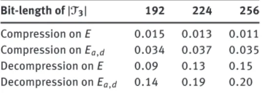
Bit-length of |T3| 192 224 256
Compression on E 0.015 0.013 0.011 Compression on Ea,d 0.034 0.037 0.035
Decompression on E 0.09 0.13 0.15 Decompression on Ea,d 0.14 0.19 0.20
Table 5. Average times for compression and decompression
on elliptic curves in short Weierstrass form and twisted Edwards curves.
Bit-length of |T3| 192 224 256
Comp on E / Comp on Ea,d 0.441 0.351 0.314
Dec on E / Dec on Ea,d 0.643 0.684 0.750
Table 6. Ratios between the average times for point
compression and decompression on elliptic curves in short Weierstrass form and twisted Edwards curves.
choose 20 000 pairs of points (P, P) of trace zero which correspond to each other via the birational isomor-phism between the curves. For each pair of points, we computeR(P), R(P), R−1(R(P)), R−1(R(P)). For each computation, we consider the average time in milliseconds for each curve, and then the averages over the five curves. The average computation times are reported in Table 5.
Table 6 contains the ratios of the average times for point compression and decompression on elliptic curves in short Weierstrass form and twisted Edwards curves.
3.2 Explicit equations, complexity, and timings for
n = 5
In this subsection we give explicit equations and perform computations for n = 5. We estimate the number of operations needed for the computations and present some timings obtained with Magma. We also make comparisons with the method proposed in [13] for elliptic curves in short Weierstrass form.
Point compression. Let P ∈ T5. By Theorem 3.4, qPis of the form
qP(x, y) = (1 + y) ̂q1(y) + xq2(y) = (1 + y)(a1y + a0) + x(b2y2+ b1y + b0),
where a0, a1, b0, b1∈ 𝔽q, and b2∈ 𝔽2. Moreover,
(1 + y)h1h2qP= ϕ1ϕ2ϕ3(a − dy2)
modulo Ea,dand up to a nonzero constant factor. We consider the generic case, where b2= 1 and ϕiis of the form
ϕi(x, y) = pi(y + 1) + x(y + qi)
with pi, qi∈ 𝔽q5and i ∈ {1, 2, 3}. Denote by k1and k2the y-coordinates of P1+ P2and P1+ P2+ P3, respec-tively. We have R(P) = (a0, a1, b0, b1, 1), where a1= k ⋅ (d(p1p2p3) + (p1+ p2+ p3)), a0= k ⋅ (3d(p1p2p3) + (p1q2+ p1q3+ q1p2+ q1p3+ p2q3+ q2p3) + (p1+ p2+ p3)) + a1⋅ (k1+ k2− 2), b1= k ⋅ (d(p1p2q3+ p1p3q2+ p2p3q1) + 2d(p1p2+ p1p3+ p2p3) + (q1+ q2+ q3)) + (k1+ k2− 1), b0= k ⋅ (2d(p1p2q3+ p1p3q2+ p2p3q1) + (d − a)(p1p2+ p1p3+ p2p3) + (q1q2+ q1q3+ q2q3) − 1) + b1(k1+ k2− 1) + (k1+ k2− k1k2), k = (d(p1p2+ p1p3+ p2p3) + 1)−1.
Computing ϕ1, ϕ2and ϕ3takes 2S+34M+2I in 𝔽q5. Computing a1, a2, b1, b0with the formulas above re-quires 45M+1I in 𝔽q5. So point compression for n = 5 takes a total of 2S+79M+3I in 𝔽q5. The method of [13] for elliptic curves in short Weierstrass form is less expensive, as it takes 3S+18M+3I in 𝔽q5.