Arctic smoke ? record high air pollution levels in the European Arctic due to agricultural fires in Eastern Europe

(1)

HAL Id: hal-00302174

https://hal.archives-ouvertes.fr/hal-00302174

Submitted on 5 Oct 2006

HAL is a multi-disciplinary open access

archive for the deposit and dissemination of sci-entific research documents, whether they are pub-lished or not. The documents may come from teaching and research institutions in France or abroad, or from public or private research centers.

L’archive ouverte pluridisciplinaire HAL, est destinée au dépôt et à la diffusion de documents scientifiques de niveau recherche, publiés ou non, émanant des établissements d’enseignement et de recherche français ou étrangers, des laboratoires publics ou privés.

Arctic smoke ? record high air pollution levels in the

European Arctic due to agricultural fires in Eastern

Europe

A. Stohl, T. Berg, J. F. Burkhart, A. M. Fjæraa, C. Forster, A. Herber, Ø.

Hov, C. Lunder, W. W. Mcmillan, S. Oltmans, et al.

To cite this version:

A. Stohl, T. Berg, J. F. Burkhart, A. M. Fjæraa, C. Forster, et al.. Arctic smoke ? record high air pollution levels in the European Arctic due to agricultural fires in Eastern Europe. Atmospheric Chemistry and Physics Discussions, European Geosciences Union, 2006, 6 (5), pp.9655-9722. �hal-00302174�

(2)

ACPD

6, 9655–9722, 2006 Arctic smoke A. Stohl et al. Title Page Abstract Introduction Conclusions References Tables Figures J I J I Back Close Full Screen / Esc

Printer-friendly Version Interactive Discussion

EGU Atmos. Chem. Phys. Discuss., 6, 9655–9722, 2006

www.atmos-chem-phys-discuss.net/6/9655/2006/ © Author(s) 2006. This work is licensed

under a Creative Commons License.

Atmospheric Chemistry and Physics Discussions

Arctic smoke – record high air pollution

levels in the European Arctic due to

agricultural fires in Eastern Europe

A. Stohl1, T. Berg1, J. F. Burkhart1,2, A. M. Fjæraa1, C. Forster1, A. Herber3, Ø. Hov4, C. Lunder1, W. W. McMillan5, S. Oltmans6, M. Shiobara7, D. Simpson4, S. Solberg1, K. Stebel1, J. Str ¨om8, K. Tørseth1, R. Treffeisen3, K. Virkkunen9,10, and K. E. Yttri1

1

Norwegian Institute for Air Research, Kjeller, Norway

2

University of California, Merced, USA

3

Alfred Wegener Institute, Bremerhaven, Germany

4

Meteorological Institute, Oslo, Norway

5

University of Maryland, Baltimore, USA

6

Earth System Research Laboratory, NOAA, Boulder, USA

7

National Institute of Polar Research, Tokyo, Japan

8

Department of Applied Environmental Science, Stockholm University, Sweden

9

Arctic Centre, University of Lapland, Finland

10

Department of Chemistry, University of Oulu, Oulu, Finland

Received: 14 September 2006 – Accepted: 2 October 2006 – Published: 5 October 2006 Correspondence to: A. Stohl (ast@nilu.no)

(3)

ACPD

EGU

Abstract

In spring 2006, the European Arctic was abnormally warm, setting new historical tem-perature records. During this warm period, smoke from agricultural fires in Eastern Europe intruded into the European Arctic and caused the most severe air pollution episodes ever recorded there. This paper confirms that biomass burning (BB) was

in-5

deed the source of the observed air pollution, studies the transport of the smoke into the Arctic, and presents an overview of the observations taken during the episode. Fire detections from the MODIS instruments aboard the Aqua and Terra satellites were used to estimate the BB emissions. The FLEXPART particle dispersion model was used to show that the smoke was transported to Spitsbergen and Iceland, which was

10

confirmed by MODIS retrievals of the aerosol optical depth (AOD) and AIRS retrievals of carbon monoxide (CO) total columns. Concentrations of halocarbons, carbon diox-ide and CO, as well as levoglucosan and potassium, measured at Zeppelin mountain near Ny ˚Alesund, were used to further corroborate the BB source of the smoke at Spitsbergen. The ozone (O₃) and CO concentrations were the highest ever observed

15

at the Zeppelin station, and gaseous elemental mercury was also enhanced. A new O₃ record was also set at a station on Iceland. The smoke was strongly absorbing – black carbon concentrations were the highest ever recorded at Zeppelin –, and strongly perturbed the radiation transmission in the atmosphere: aerosol optical depths were the highest ever measured at Ny ˚Alesund. We furthermore discuss the aerosol

chem-20

ical composition, obtained from filter samples, as well as the aerosol size distribution during the smoke event. Photographs show that the snow at a glacier on Spitsber-gen became discolored during the episode and, thus, the snow albedo was reduced. Samples of this polluted snow contained strongly enhanced levels of potassium, sul-phate, nitrate and ammonium ions, thus relating the discoloration to the deposition of

25

the smoke aerosols. This paper shows that, to date, BB has been underestimated as a source of aerosol and air pollution for the Arctic, relative to emissions from fossil fuel combustion. Given its significant impact on air quality over large spatial scales and on

(4)

ACPD

EGU radiative processes, the practice of agricultural waste burning should be banned in the

future.

1 Introduction

The European sector of the Arctic saw unprecedented warmth during the first months of the year 2006. At Ny ˚Alesund on the island of Spitsbergen in the Svalbard archipelago,

5

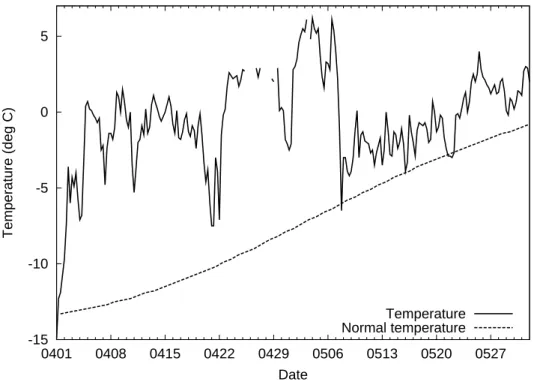
the monthly mean temperatures from January to May were 10.7, 3.8, 1.4, 10.3, and 4.2◦C above the corresponding values averaged over the period since 1969 (Mete-orological Institute, 2006); the January, April and May values were the highest ever recorded. Figure1, a comparison between the temperatures measured at Ny ˚Alesund in April and May 2006 with the corresponding climate mean, shows that the entire two

10

months were warmer than normal. Due to the abnormal warmth, the seas surround-ing the Svalbard archipelago were almost completely free of closed ice at the end of April, for the first time in history. In contrast to the Arctic, the European continent saw a delayed onset of spring in 2006. Snow melt in large parts of Europe occurred only in April; even as late as 1 May, snow covered much of Scandinavia.

15

Related to the abnormal warmth in the Arctic, record-high levels of air pollution were measured at the Zeppelin station near Ny ˚Alesund on Spitsbergen. It will be shown in this paper that they were caused by transport of smoke from agricultural fires in Eastern Europe. These fires were started later than normal because of the late snow melt. The most severe air pollution episodes happened on 27 April and during the first days of

20

May 2006 when the concentrations of most measured air pollutants (aerosols, O₃, etc.) exceeded the previously recorded long-term maxima. Views from the Zeppelin station clearly showed the decrease in visibility from the pristine conditions on 26 April to when the smoke engulfed Svalbard on 2 May (Fig.2). Iceland, where a new O₃record was set at the Storhofdi station, was also affected by the smoke plume.

(5)

ACPD

EGU

2 Arctic air pollution

Because of its remoteness, the Arctic troposphere was long believed to be extremely clean but in the 1950s, pilots flying over the North American Arctic discovered a strange haze (Greenaway,1950;Mitchell,1957), which decreased visibility significantly. The Arctic Haze, accompanied by high levels of gaseous air pollutants (e.g., hydrocarbons;

5

Solberg et al.,1996), was observed regularly since then and is a result of the special meteorological situation in the Arctic in winter and early spring (Shaw,1995). Temper-atures at the surface become extremely low, leading to a thermally very stable stratifi-cation with frequent and persistent occurrences of surface-based inversions (Bradley, 1992) that reduce turbulent exchange, hence dry deposition. The extreme dryness

min-10

imizes wet deposition, thus leading to very long aerosol lifetimes in the Arctic in winter and early spring. After polar sunrise, photochemical activity increases and can pro-duce phenomena such as the depletion of O₃and gaseous elemental mercury (GEM) (Lindberg et al.,2002).

Surfaces of constant potential temperature form closed domes over the Arctic, with

15

minimum values in the Arctic boundary layer (Klonecki et al., 2003). This transport barrier isolates the Arctic lower troposphere from the rest of the atmosphere. Me-teorologists realized that in order to facilitate isentropic transport, a pollution source region must have the same low potential temperatures as the Arctic Haze layers (Carl-son, 1981; Iversen, 1984; Barrie, 1986). For gases and aerosols with lifetimes of a

20

few weeks or less, this rules out most of the world’s pollution source regions because they are too warm, and leaves northern Eurasia as the main source region for the Arctic Haze (Rahn,1981;Barrie,1986;Stohl,2006). Transport from Eurasia is highly episodic and is often related to large-scale blocking events (Raatz and Shaw,1984; Iversen and Joranger,1985).

25

Boreal forest fires are another large episodic source of Arctic air pollutants, particu-larly of black carbon (BC) (Lavou ´e et al.,2000), which has important radiative effects in the Arctic, both in the atmosphere and if deposited on snow or ice (Hansen and

(6)

ACPD

EGU Nazarenko,2004). They occur in summer when wet and dry deposition are relatively

efficient and the Arctic troposphere is generally cleaner than in winter. Nevertheless, an aircraft campaign in Alaska frequently sampled aerosol plumes from Alaskan and maybe also Siberian forest fires (Shipham et al., 1992), and a PhD thesis suggests that BC observations at Arctic sites are linked to boreal forest fires (Lavou ´e,2000).

Re-5

cently,Stohl et al.(2006) showed that severe forest fires burning in Alaska and Canada led to strong pan-Arctic increases in light absorbing aerosol concentrations during the summer of 2004.

In this paper, we identify another source of Arctic air pollution, namely agricultural fires. We will analyze the transport of the pollution plumes into the Arctic and present

10

an overview of aerosol and air chemistry measurements made during the most extreme air pollution episode ever recorded at Svalbard and Iceland.

3 Observations

We present measurements mostly from the research station Zeppelin (11.9◦E, 78.9◦N, 478 m a.s.l.). The station is situated in an unperturbed Arctic environment on a ridge

15

of Zeppelin mountain on the western coast of Spitsbergen. Because of the altitude difference and the generally stable atmospheric stratification, contamination from the nearby small settlement of Ny ˚Alesund (located near sea level) is minimal at Zeppelin. Hourly O₃concentrations were recorded by UV-absorption spectrometry (API 400A). GEM was measured using a Tekran gas phase mercury analyzer (model 2537A) as

de-20

scribed inBerg et al.(2003). CO was measured using a RGA3 analyzer (Trace Analyti-cal) fitted with a mercuric oxide reduction gas detector. Five ambient air measurements and one field standard were performed every 2 h. The field standards were referenced against a Scott-Marine Certificated standard and a calibration scale (Langenfelds et al.,1999;Francey et al.,1996).

25

Carbon dioxide (CO₂) was measured using a Non-dispersive Infrared Radiometer (NDIR), Li-COR model 7000. The radiometer was run in differential mode using a

(7)

ACPD

EGU reference gas with a CO₂ content near the measured concentrations. Roughly every

2 h the radiometer was calibrated using three different CO₂ concentrations spanning the expected atmospheric concentration interval. Halocarbons were analyzed by gas chromatography/mass spectroscopy (Agilent, 5793N) at 4-hourly intervals. Substances from 2 l of air were preconcentrated on an automated adsorption-desorption system

5

filled with three different adsorbents. This preconcentration unit was developed by the University of Bristol (Simmonds et al.,1995) and has been in operation in the AGAGE network for several years (Prinn et al.,2000).

The particle size distributions were measured using a Differential Mobility Particle Sizer (DMPS) consisting of a Differential Mobility Analyser (Knutson and Whitby,1975)

10

and a TSI 3010 particle counter. The sheath flow is a closed-loop system (Jokinen and Makela,1997). DMPS data from Zeppelin have been presented previously (Str ¨om et al.,2003) and cover the size range from 13.5 to 700 nm diameter (bin limits).

Information on light absorbing particles was gathered with a custom-built particle soot absorption photometer (PSAP). In this instrument, light at 530 nm wavelength

illu-15

minates two 3 mm diameter spots on a single filter substrate, on one of which particles are collected from ambient air flushed through the filter, and the other kept clean as a reference. The change in light transmittance across the filter is measured to derive the particle light absorption coefficient σ_ap, ignoring the influence of scattering particles. Conversion of σ_ap to BC concentrations requires the assumptions that all the light

ab-20

sorption measured is from BC, and that all BC has the same light absorption efficiency. We convert σ_ap values to equivalent BC (EBC) mass concentrations using a value of 10 m2g−1, typical of aged BC aerosol (Bond and Bergstrom,2005).

Aerosol filter samples were collected for subsequent analysis of the aerosols’ con-tent of anions (Cl−, NO−₃, SO2−₄ ) and cations (Ca2+, Mg2+, K+, Na+, NH+₄) on a daily

25

basis using an open face NILU filter holder, loaded with a 47 mm diameter Teflon filter (Zefluor 2 µm). The cations and anions were quantified by ion chromatography. While NO−₃ and NH+₄ are subject to both positive and negative biases, we only report the sum of particulate and gaseous phases for the two. For conditions typical for Norway,

(8)

ACPD

EGU the particulate phase is the dominant fraction accounting for 80–90% of NO−₃ and

ap-proximately 90% of NH+₄. Aerosol samples were also collected on 800×1000 cellulose filters (Whatman 41) according to a 2+2+3 days weekly sampling scheme, using a high volume sampler with a 2.5 µm cut off. Using these samples, the aerosols’ content of levoglucosan was analyzed with high performance liquid chromatography combined

5

with time-of-flight high-resolution mass spectrometry (HPLC/HRMS) as described by Dye and Yttri(2005). Finally, weekly aerosol samples were collected using a Leckel SEQ47/50 sampler loaded with prefired quartz fibre filters. The samples’ content of elemental carbon (EC) and organic carbon (OC) was quantified using the NIOSH 5040 thermo-optical method (Birch and Cary,1996), which accounts for pyrolytically

gener-10

ated EC during the analysis.

At Ny ˚Alesund, daylight measurements of the spectral aerosol optical depth (AOD) were made with the automatic sun photometer SP1A which uses the imaging method ofLeiterer and Weller(1988). Seventeen channels cover the spectral range from 350 to 1065 nm with a full-width-half-maximum of 5 to 15 nm. The accuracy of the measured

15

AOD is between 0.005 and 0.008. The measurement time is less than 5 s but the data presented here are hourly mean values. More details can be found in Herber et al. (2002).

A Micro-Pulse Lidar Network (MPLNET) instrument (Welton et al.,2001) is operated for the National Institute of Polar Research (Japan) at Ny ˚Alesund by the Alfred

We-20

gener Institute for Polar and Marine Research, Germany, since 2002. The MPL uses a Nd/YLF laser, emitting laser light at a wavelength of 523.5 nm. Details regarding on-site maintenance, calibration techniques, description of the algorithm used and data products are given in Campbell et al. (2002). We present the corrected normalized relative backscatter signal, which corresponds to the raw signal counts from the MPL,

25

processed to remove all instrument related parameters except the calibration constant. Since the molecular return gives rise to a range-corrected signal decrease of 50% be-tween ground and 5 km altitude due to the molecular density decrease, we normalized the relative backscatter with the molecular return using a standard-atmospheric density

(9)

ACPD

EGU profile. The data are stored at 1 min time resolution and 30 m vertical resolution.

In addition to the measurements from Spitsbergen, we also present surface O₃ mea-surements from Storhofdi (20.34◦W, 63.29◦N, 127 m asl) on the southernmost tip of the island of Heimay in the Westman Islands, a group of small volcanic islands to the south of the principal island of Iceland. The preponderance of airflow is from off the

5

Atlantic Ocean and there is only a small population center about 5 km north of the measurement site. Ozone measurements are made using a Thermo Environmental Instruments (TEI) model 49C analyzer, which has been regularly intercompared with a secondary standard O₃ analyzer maintained by the NOAA Earth System Research Laboratory, Global Monitoring Division. This secondary standard is calibrated against

10

a standard reference O₃photometer maintained by the U.S. NIST.

For studying the transport and geographical extent of the aerosol pollution, we also used satellite measurements. Total column CO was retrieved from the Atmospheric InfraRed Sounder (AIRS) in orbit onboard NASA’s Aqua satellite. All AIRS retrievals for the given days were binned to a 1×1◦ grid. The prelaunch AIRS CO retieval algorithm

15

was employed using the AFGL standard CO profile as the first guess and the AIRS team retrieval algorithm PGE v4.0. Although AIRS CO retrievals are most sensitive to the mid-troposphere, the broad averaging kernel can be influenced by enhanced CO abundances near the boundary layer (McMillan et al.,2005, 20061).

The daily level 3 AOD data at a wavelength of 550 nm, retrieved with algorithm

20

MOD08 D3 from the MODIS Terra Collection 4, were also used. A description and validation of these data can be found inRemer et al. (2005) andIchoku et al.(2005). Their stated accuracy is ±(0.05+0.2×AOD) over land and ±(0.03+0.05×AOD) over ocean. Retrievals are not being made in cloudy areas, or in regions with a high surface

1

McMillan, W. W., Warner, J. X., McCourt Comer, M., Maddy, E., Chu, A., Sparling, L., Eloranta, E., Hoff, R., Sachse, G., Barnet, C., Razenkov, I., and Wolf, W.: AIRS views of transport from 10–23 July 2004 Alaskan/Canadian fires: Correlation of AIRS CO and MODIS AOD and comparison of AIRS CO retrievals with DC-8 in situ measurements during INTEX-NA/ICARTT, J. Geophys. Res., submitted, 2006.

(10)

ACPD

EGU albedo, e.g. over most of snow-covered Norway, and in ice-covered parts of the Arctic.

4 Biomass burning emissions

In April and May 2006, a large number of fires occurred in the Baltic countries, west-ern Russia, Belarus, and the Ukraine. The fires were started by farmers who burned their fields before the start of the new growing season. This practice is illegal in the

5

European Union but is still widely used in Eastern Europe for advancing crop rotation and controlling insects and disease. It is quite common that agricultural fires get out of control and devastate nearby forests or human property. According to newspaper reports (seehttp://www.baltictimes.com), the fires burned into the forests of the nature preserve Kuronian Spit in Lithuania and could be extinguished only after considerable

10

efforts. Five people died in the fires in Latvia.

For estimating biomass burning (BB) emissions from these fires, we used ac-tive fire detections by the MODIS instruments onboard the Aqua and Terra satel-lites. These detections are based on MODIS Collection 4 data and the MOD14 and MYD14 algorithms (Giglio et al.,2003) (see http://maps.geog.umd.edu/products/

15

MODIS Fire Users Guide 2.2.pdf). A number between 0 and 100 characterizes the confidence for every fire detection. We only used detections with a confidence level greater than 75. The algorithm uses data from pixels of about 1 km2size but the actual fire size is not known. Fires of 1000 m2or less can be detected under good observing conditions but even large fires can be obscured by clouds. Furthermore, detections

20

can only be made at the time of the satellite overpasses and the number of detections also depends on the minimum confidence level requested. In the absence of better in-formation, we assumed that every detection represents a burned area of 180 ha, based on a statistical analysis of MODIS fire detections with independent area burned data byWotawa et al.(2006). This shall account both for the area burned by the detected

25

fire itself and undetected fires in its vicinity on the same day.

(11)

ACPD

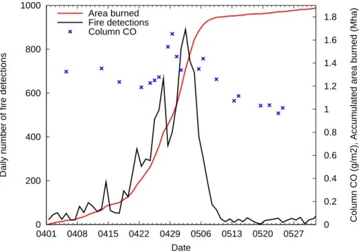
EGU between 20 and 60◦E. More than 300 fires/day were detected from 25 April to 6 May

2006, with a peak of more than 800 detections on 2 May. This leads to an estimate of almost 2 million hectare burned in April and May 2006. The decrease in the number of fire detections on 28–30 April is likely not due to an actual decrease in fire activity but to the presence of clouds near 32◦E and 54◦N. In a crude attempt to account for the

5

cloud effect on 28–30 April, we doubled the fire pixels in a small area to the northeast of the clouds and shifted these “shadow” pixels to the southwest into the cloud band. This increased the number of detections by about 40% on 28 and 29 April and 10% on 30 April.

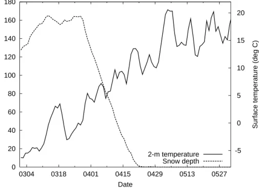
Figure 4 shows time series of the surface temperature and snow depth (shown as

10

mm water equivalent), averaged over the region where most of the fires burned. There was a lot of snow on the ground until the end of March, which started melting in April. The fire frequency increased dramatically on 21 April (see Fig. 3), after all the snow had disappeared. Korontzi et al.(2006) show that spring-time agricultural burning in Eastern Europe peaked in March in the year 2002 and in April in the years 2001 and

15

2003, whereas in all three years there was very little burning in May. In 2002, a smoke episode caused by agricultural fires in this region was observed in Finland already in the middle of March (Niemi et al.,2004). In 2006, in contrast, farmers were forced to wait with the burning for the unusually late snow melt, causing a strong emission pulse at the end of April/beginning of May (see Fig.3) when fields were quickly prepared for

20

the already delayed sowing. This is demonstrated also by the infrared spectroscopy measurements of total column CO made at Zvenigorod (36◦E, 55◦N; see Yurganov et al., 1995), which is located about 50 km west of Moscow and within the general burning region (symbols in Fig. 3). Superimposed on the seasonal decrease from winter to summer, there is a pronounced peak of total column CO at about the time of

25

the maximum fire occurrence. In other years, the CO variability was smaller and no late spring maximum was observed.

(12)

equa-ACPD

EGU tion

E = ABαβ (1)

where A is the area burned, B is the biomass per area, α is the fraction of the biomass consumed by the fire, and β is the CO emission factor. Every detected fire was linked to a certain land cover type, using a global land cover classification with a resolution

5

of 1 km (Hansen et al., 2000). Figure 5 shows a map of the MODIS fire detections between 21 April and 5 May as a function of land cover. The percentage of fires detected, the factors B, α and β used for the emission calculation, and the estimated emissions are reported in Table 1 for the various land cover types. The values of B and α are similar to those recently used byWiedinmyer et al.(2006); values of β were

10

taken fromAndreae and Merlet(2001). The majority (55%) of the fires were detected in cropland, 24% in wooded grassland, 8% in woodland, 7% in grassland, and 5% in forests. Because of the low fuel loading in cropland, emissions there were only 21% of the total, whereas wooded grassland contributed 36%, woodland 12%, grassland 4%, and forests 26%.

15

It must be cautioned that our emission estimates are highly uncertain. We estimate that the total area burned is uncertain by at least a factor of two. We furthermore expect the attribution of fires to land cover types other than croplands to be biased high. In a pixel with a mosaic of different land cover types including croplands, a detected fire is most likely burning on agricultural fields, since the fires were started by farmers.

20

Our algorithm, however, attributes it to the dominant land cover type. Assuming that all fires actually burned on agricultural fields would lead to 60% lower total emissions. Additional uncertainties are associated with the factors B, α and β, such that the overall uncertainty of the BB emission estimate is at least a factor of three.

In addition to the BB emissions, we also used CO emissions from fossil fuel

com-25

bustion (FFC) sources. For Europe, we used the expert emissions taken from the UNECE/EMEP (United Nations Economic Commission for Europe/Co-operative Pro-gramme for Monitoring and Evaluation of Long Range Transmission of Air Pollutants in Europe) emission database for the year 2003. These data are based on official country

(13)

ACPD

EGU reports with adjustments made by experts (Tarrason et al.,2005) and are available at

0.5◦ resolution from http://www.emep.int. The emissions were uniformly reduced by 10% to account for a likely reduction of European CO emissions since 2003. Emis-sions elsewhere were taken from the EDGAR 3.2 Fast Track 2000 dataset (Olivier et al.,2001).

5

5 Model simulations

Simulations of air pollution transport were made using the Lagrangian particle dis-persion model FLEXPART (Stohl et al., 1998,2005;Stohl and Thomson,1999) (see http://zardoz.nilu.no/∼andreas/flextra+flexpart.html). FLEXPART was validated with data from continental-scale tracer experiments (Stohl et al.,1998) and was used

pre-10

viously to study the transport of BB emissions to downwind continents (Forster et al., 2001; Damoah et al., 2004) and into the Arctic (Stohl et al., 2006), as well as the transport of FFC emissions between continents (Stohl et al.,2003) and into the Arctic (Eckhardt et al., 2003). FLEXPART is a pure transport model and no removal pro-cesses were considered here. The only purpose of the model simulations is to identify

15

the sources of the measured pollution.

FLEXPART was driven with analyses from the European Centre for Medium-Range Weather Forecasts (ECMWF,2002) with 1◦×1◦resolution (derived from T319 spectral truncation) and two nests (108◦W–27◦W, 9◦N–54◦N; 27◦W–54◦E, 35◦N–81◦N) with 0.36◦×0.36◦resolution (derived from T799 spectral truncation). In addition to the

anal-20

yses at 00:00, 06:00, 12:00 and 18:00 UTC, 3-h forecasts at 03:00, 09:00, 15:00 and 21:00 UTC were used. There are 23 ECMWF model levels below 3000 m, and 91 in total. We also made alternative FLEXPART simulations using input data from the Na-tional Centers for Environmental Prediction Global Forecast System (GFS) model with 1◦×1◦resolution and 26 pressure levels.

25

FLEXPART calculates the trajectories of so-called tracer particles using the mean winds interpolated from the analysis fields plus random motions representing

(14)

turbu-ACPD

EGU lence. For moist convective transport, FLEXPART uses the scheme ofEmanuel and

ˇ

Zivkovi´c-Rothman (1999), as described and tested by Forster et al. (2006). In order to maintain high accuracy of transport near the poles, FLEXPART advects particles on a polar stereographic projection poleward of 75◦ but using the ECMWF winds on the latitude-longitude grid to avoid unnecessary interpolation. A special feature of

FLEX-5

PART is the possibility to run it backward in time (Stohl et al.,2003;Seibert and Frank, 2004).

For this study, FLEXPART was run both forward from the emission fields and back-ward in time from the Zeppelin station. The purpose of the forback-ward simulation was to identify the areas affected by the BB emissions and to understand the transport in

rela-10

tion to the synoptic conditions. 13 million tracer particles of equal mass were released from the fire locations, with the number of particles used depending on a fire’s calcu-lated emission strength. The particles were injected between 0 and 100 m above the surface, as satellite images show that the agricultural fires did not trigger substantial pyro-convection. Forward tracer simulations were also made for FFC CO emissions

15

from Europe, North America and Asia, respectively.

Backward simulations from Zeppelin were made for 3-h time intervals in April and May 2006. For each such interval, 40 000 particles were released at the measurement point and followed backward in time for 20 days, forming what we call a retroplume, to calculate a potential emission sensitivity (PES) function, as described bySeibert and

20

Frank (2004) and Stohl et al. (2003). The word “potential” indicates that this sensi-tivity is based on transport alone, ignoring removal processes that would reduce the sensitivity. The value of the PES function (in units of s kg−1) in a particular grid cell is proportional to the particle residence time in that cell. It is a measure for the simulated mixing ratio at the receptor that a source of unit strength (1 kg s−1) in the respective

25

grid cell would produce. For consistency with the forward simulations, we report PES values for a so-called footprint layer 0–100 m above ground. Folding (i.e., multiplying) the PES footprint with the emission flux densities (in units of kg m−2s−1) from the FFC and BB inventories yields so-called potential source contribution (PSC) maps, that is

(15)

ACPD

EGU the geographical distribution of sources contributing to the simulated mixing ratio at

the receptor. Spatial integration finally gives the simulated mixing ratio at the receptor. Time series of these mixing ratios, obtained from the series of backward simulations, will be presented both for FFC and BB emissions. Since the backward model output was generated daily, the timing of the contributing emissions is also known.

5

6 Pollution transport to the Arctic

The meteorological situation in the northern hemisphere in late April and beginning of May was characterized by so-called low-zonal-index conditions with large waves in the middle latitudes and generally weak westerly winds. The waves produced strong undulations of the jet stream and caused large meridional exchange of air. This can be

10

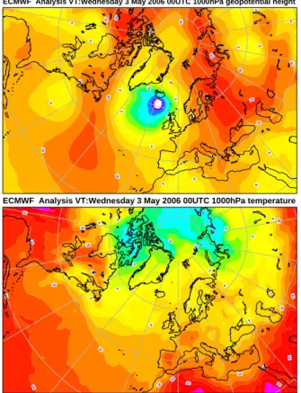
seen in Fig.6(top), which shows the situation on 3 May at 00:00 UTC, approximately at the time with the highest pollution levels measured at Spitsbergen. There were several strong high- and low-pressure centers in the northern hemisphere. The Icelandic low dominated the circulation over the northern North Atlantic and a prominent anticyclone was located over northeastern Europe. This pressure configuration corresponds to

15

a strongly positive phase of the North Atlantic Oscillation pattern, which is known to enhance pollution transport into the Arctic (Eckhardt et al., 2003). Consequently, air from the European continent was channelled into the Arctic between the two pressure centers, leading to abnormally high temperatures over the Norwegian and Barents Seas and the Arctic Ocean (see Fig. 6, bottom). The situation on 25–27 April (not

20

shown) was similar. Indeed, the first pulse of smoke arrived at Spitsbergen already on 27 April. Between the two episodes, the eastern European high connected with the Azores high, pushing the Icelandic low further north and interrupting the northward flow for two days. This also brought some precipitation to Svalbard on 28 and 29 April (4 and 9 mm at Ny ˚Alesund). After 3 May, the anticyclone over Eastern Europe grew and

25

extended further to the west. On 7 May, it stretched into the Norwegian Sea, such that air from Europe was first transported westward to the British Isles, and then around

(16)

ACPD

EGU the high and to the north. Still later, the high’s center moved to Greenland, and the

European outflow reached Iceland but not anymore Svalbard. While no precipitation was measured on Svalbard during the first days of May, the episode was ended by a cold front bringing rain and snow (1, 4 and 7 mm precipitation at Ny ˚Alesund on 6, 7, and 8 May) and finally clean Arctic air masses to the archipelago (Meteorological

5

Institute,2006).

The meteorological situation is reminiscent of the conditions when Arctic Haze is ob-served at Svalbard in winter and early spring. Like during Arctic Haze episodes the flow from the Eurasian continent was channelled northward between a cyclone and an anticyclone in a low-zonal-index situation. However, during Arctic Haze the anticyclone

10

is typically located further east (Iversen, 1984; Iversen and Joranger, 1985), due to the low temperatures in Siberia in winter. In April/May 2006, the transport of pollution from Eastern Europe to Svalbard and Iceland was possible only because of the unusu-ally high temperatures in the Arctic, which basicunusu-ally eliminated the polar dome (Stohl, 2006). Thus, instead of the pollution source region being extremely cold as it occurs

15

during Arctic Haze, the Arctic receptor region became unusually warm in spring 2006. Should the warming of the Arctic continue to proceed more quickly than that of the middle latitudes, such transport conditions may become more frequent in the future.

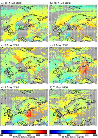
To illustrate the transport of the smoke from the fires in Eastern Europe, we show maps of the total column BB CO tracer from the FLEXPART forward simulation, with

20

superimposed MODIS AOD values, for the period 29 April-7 May (Fig.7). AOD iso-lines are not closed where retrievals were not successful over snow-covered parts of Scandinavia, Arctic ice, and near clouds. We also compare the model results to CO retrievals from AIRS (Fig.8). On 29 April (Fig.7a), the plume stretched from the fire re-gion where maximum AOD values were about 1.3 units, northwestward to Scandinavia.

25

The close correspondence between the FLEXPART passive tracer simulation and the MODIS AOD field suggests that aerosols were not removed from the atmosphere to a significant extent, and that the aerosol distribution over Europe was dominated by the BB emissions. CO retrievals from AIRS (Fig.8a) also show the highest values over the

(17)

ACPD

EGU fire region but weaker spatial gradients.

One day later, on 30 April (Fig. 7b and8b), the pollution plume reached the Nor-wegian Sea, and on 2 May (Fig.7c and8c), it had already arrived at Svalbard. AOD retrievals were not successful around Svalbard but values up to 1.5 units can be found a few degrees east of it (Fig.7c). On 2 May, this plume is also the most prominent

5

feature in the AIRS map (Fig.8c). The retrieved CO enhancement over the Norwegian Sea (about 200 mg m−2 above the background of about 1000 mg m−2) compares well with the FLEXPART BB CO tracer values in this region.

On 3 May, both the FLEXPART BB CO and AIRS CO show a dramatic increase over Eastern Europe, following the peak in the number of fire detections on 2 May.

10

The roughly 400 mg m−2CO enhancement above the background seen by AIRS again agrees well with the FLEXPART BB CO in the fire region. The plume was still present around Spitsbergen on 3 (Fig. 7d and 8d) and 4 May but then moved further to the northeast and was replaced by somewhat cleaner air on 5 and 6 May. On 5 May (Fig.7e), a band of high AOD values (up to about 0.8 units) extended northwestwards

15

from the British Isles. This band is not associated with BB CO tracer but can be seen in the FFC CO tracer simulation (not shown) and, thus, can be attributed to the export of pollution from Western Europe. AOD maxima also occur southwest of Spitsbergen (near 0◦W and 75◦N) where the FFC plume arrived on 6 May.

On 7 May (Fig.7f), the BB plume was exported into the North Atlantic and arrived

20

at Iceland on 8 May (not shown). This part of the plume did not reach Spitsbergen anymore where a change in wind direction replaced the polluted warm air with clean Arctic air (see the temperature drop in Fig. 1). Relatively high CO columns are still seen by AIRS over the Norwegian and Barents Sea on 5–7 May (Fig. 8e–f), which FLEXPART attributes mostly to FFC in Europe (not shown; but see Fig.10, explained

25

later).

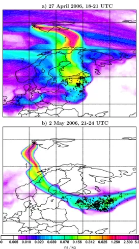
Figure 9shows PES footprints of the retroplumes from the Zeppelin station for two 3-h intervals, 27 April 18:00–21:00 UTC and 2 May 21:00–24:00 UTC, during the two main observed pollution episodes. Fire detection locations are superimposed on the

(18)

ACPD

EGU PES footprint maps in regions where and only for days on which the daily PES

foot-print value exceeds 5 ps kg−1. For 27 April (Fig.9a), the retroplume travels northward from Eastern Europe and converges towards the station from the east. The high PES footprint values (yellowish colors) extend into the area where many fires were detected when the air passed over it 3–4 days before its arrival at Zeppelin. For 2 May 21:00–

5

24:00 UTC (Fig.9b), the retroplume is more narrow and, in fact, the PES maps for 2, 3, and 4 May are all similar, with the retroplumes coming from Eastern Europe and passing over Scandinavia. The air traveled over many fires 2–5 days before arriving at Zeppelin and picked up copious amounts of BB emissions. The air was also contam-inated with FFC emissions, mostly from around Moscow according to the PSC map

10

(not shown). However, the total FFC CO is only 10 ppb, much less than the simulated BB CO of 72 ppb and the observed CO enhancement of about 100 ppb.

Figure10 shows time series of the simulated CO tracer mixing ratios from all back-ward simulations between 24 April and 9 May. Simulated CO tracers are shown for BB (Fig. 10a) and FFC (Fig.10b), BB+FFC (Fig.10c), and BB+FFC obtained when

15

using the alternative GFS analyses for driving FLEXPART (Fig.10d). In all panels, the observed CO is shown as a black line. The previously highest 2-h mean CO mixing ratio measured at the station since the year 2001 of 230 ppb was exceeded on 2 and 3 May. Since simulated CO tracers accumulated emissions only over 20 days, they do not reproduce the observed CO background of about 140 ppb. However, the episodes

20

of enhanced CO are well captured by the sum of BB and FFC CO tracers. There are subtle differences between the two simulations using ECMWF and GFS data (e.g., the GFS simulation overestimates the CO peak on 27 April, whereas the ECMWF simu-lation overestimates the largely anthropogenic CO peak on 7 May) but generally both model versions reproduce the observed CO variations reasonably well. Both show

25

a first pollution episode on 27 April, then a break, a strong episode from 1–5 May, followed by cleaner periods and weaker episodes on 6 and 7 May.

According to both model versions, BB emissions were always mixed with FFC emis-sions, which is not surprising given that the fires were burning in densely populated

(19)

ACPD

EGU areas. There were some periods when FFC emissions dominated, e.g., on 6 and 7

May, but both model versions attribute most of the CO enhancement during the main episode from 1–5 May to BB. However, it is important to keep in mind that the relative contributions of FFC and BB emissions can be very different for species other than CO. According to FLEXPART, the BB plume was traveling at altitudes below 3 km at all

5

times. This is confirmed by plots of the corrected normalized relative backscatter signal from the micropulse lidar at Ny ˚Alesund (Fig.11), which shows strong returns mostly below 2 km. On 2 May and on 3 May in the morning, when the highest pollution levels were measured at Zeppelin, the smoke aerosol concentrations decreased with altitude and the station was in the densest part of the plume. However, on 3 May in the

after-10

noon, the smoke was more dense aloft. This is captured by the FLEXPART BB CO tracer simulation and also confirmed by an ozonesonde launched from Ny ˚Alesund on 3 May, which shows increasing O₃ mixing ratios up to 2 km and a decrease at about 2.4 km (see Fig.15, discussed later). On average, the smoke observed at Ny ˚Alesund had a layer thickness of about 2 km and, thus, filled a significant part of the troposphere.

15

7 Air chemistry and aerosol observations

7.1 Halocarbons

The hydrofluorocarbons HFC-134a and HFC-152a (atmospheric lifetimes of 14 and 1.4 years, respectively) are used as refrigerants and blowing agents for producing in-solation foams (WMO,2005). Since they have no natural sources, they are excellent

20

tracers for emissions from anthropogenic activities. At remote observatories, distinct peaks of HFC-134a and HFC-152a concentrations occur when air masses from major population centers are transported to the station (Reimann et al.,2004). Even though HFC-134a and HFC-152a are not themselves emitted by FFC, their regional emission patterns correlate with those of FFC, such that they can help identifying when

pollu-25

(20)

ACPD

EGU mostly natural sources, including BB (Khalil and Rasmussen,1999,2003).

Figure 12 shows HFC-134a, HFC-152a, and CH₃Cl measurements superimposed on the time series of measured CO. Instrument maintenance work was performed at the end of April/beginning of May, such that the data record is unfortunately not com-plete but still sufficient for our purpose. The anthropogenic tracers 134a and

HFC-5

152a both have their highest values on 27 April and 6 May, at times when FLEXPART suggests relatively strong FFC episodes (see Fig.10). The enhancements during the main CO episode from 1–5 May are much smaller. HFC-134a values are higher at the beginning (2 May) and at the end (5 May) of this period than in its middle (3–4 May), in agreement with the FLEXPART FFC CO tracer concentrations (Fig.10). On the other

10

hand, CH₃Cl is well correlated with CO in the BB plume. The peak enhancement above the background on 3 May of about 30 pptv corresponds to an enhancement ratio (ER) of 0.0003, relative to the 100 ppb CO enhancement. This is consistent with reported CH₃Cl/CO emission ratios from vegetation fires (Andreae and Merlet,2001). In sum-mary, this confirms that at Zeppelin CO was dominated by BB emissions, whereas FFC

15

emissions played a smaller role. 7.2 Carbon dioxide

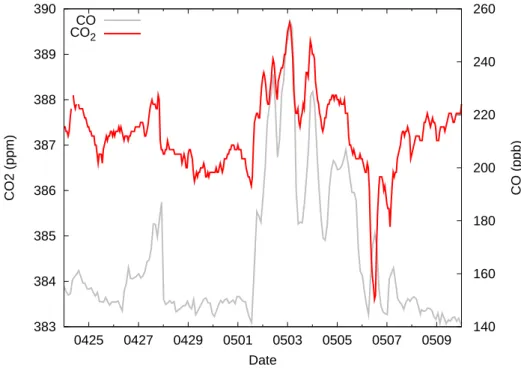
Figure13 compares time series of CO₂ and CO. The two species co-variate from 24 April–5 May but are anti-correlated later on. The likely reason for the anti-correlation during the FFC episodes on 6 and 7 May is that the source regions for these episodes

20

are in Western Europe where the vegetation was already active and took up more CO₂ than what was emitted by FFC. However, during the major BB episode, CO and CO₂are highly correlated, thus facilitating a regression analysis. Since CO data were available as two-hour means with irregular starting times, every CO value was assigned the 1-hourly CO₂value that fell entirely into the CO sampling interval. Standard linear

25

regression analysis with CO₂as the independent variable resulted in a CO/CO₂slope of 0.023 (after conversion to mass mixing ratios) and a Pearson correlation coefficient of 0.91 for the period 1–4 May. In comparison, average CO/CO₂emission ratios from

(21)

ACPD

EGU passenger cars range from 0.002–0.016 (Vasic and Weilenmann,2006) and, according

to the EDGAR inventory, Germany’s overall CO/CO₂ emission ratio in the year 2000 was about 0.006. Agricultural fires have a much higher CO/CO₂emission ratio of 0.06 with an uncertainty of a factor of two (Andreae and Merlet,2001). Assuming CO/CO₂ emission ratios of 0.006 and 0.06 for FFC and BB emissions, respectively, the observed

5

CO/CO₂ slope of 0.023 indicates that 35% of the CO₂ and 82% of the CO variability during 1–4 May were due to BB.

7.3 Ozone

The peak O₃ mixing ratios during both episodes clearly exceeded the previously set long-term (since 1989) record-high 1-h-mean mixing ratio of 61 ppb at the Zeppelin

10

station and set a new record of 83 ppb (Fig.14). An ozonesonde launched on 3 May at 11:00 UTC measured increasing O₃mixing ratios with altitude up to some 2400 m a.s.l., above which O₃decreased sharply at a temperature inversion that capped the polluted layer (Fig.15).

In order to explore whether the extremely high O₃levels were due only to the high

15

loads of precursor substances or also to especially effective O₃ formation, we per-formed standard linear regression analyses with measured CO as the independent variable, for the three periods marked in Fig.14, and for the remaining April–May data. As described before for CO₂, every 2-hourly CO value was assigned a 1-hourly O₃ value. Figure16shows a scatter plot of O₃versus CO data for the different time

peri-20

ods, with regression lines drawn through the data, and Table2 reports the regression parameters. Overall, there is a positive O₃-CO correlation in April–May 2006, which is indicative of a regime dominated by photochemical O₃formation. Note that a negative O₃-CO correlation would be expected for air masses originating in the stratosphere but stratospheric air masses cannot normally descend into the Arctic polar dome (Stohl,

25

2006). Pearson correlation coefficients for the three periods range from 0.84–0.87, indicating compact positive O₃-CO relationships.

(22)

in-ACPD

EGU form about the number of O₃ molecules formed per CO molecule emitted, assuming

that both CO and O₃ are conserved during transport. For aged North American FFC plumes in the North Atlantic region in summer, Parrish et al. (1998) reported aver-age O₃-CO slopes of 0.25–0.40, with values up to 1.0 for individual plumes. For the Azores, an average slope of 1.0 was reported for summer conditions (Honrath et al.,

5

2004). For aged BB plumes, O₃-CO slopes are normally less steep, which is due to the lower NO_x/CO emission ratios of BB compared to FFC and, thus, less efficient O₃ formation per CO molecule. Over Alaska,Wofsy et al. (1992) found average O₃-CO slopes of 0.1 in BB plumes; downwind of North American boreal forest fires, Real et al. (2006)2reported small negative to small positive values;Wotawa and Trainer(2000)

10

found small positive slopes of 0.05–0.11 in BB plumes transported from Canada to the eastern United States; for the Azores, Honrath et al.(2004) reported a range of 0.4– 0.9 for plumes from boreal forest fires (with contributions from FFC); andAndreae et al. (1994) reported slopes of 0.46±0.23 for BB plumes over the tropical South Atlantic. The O₃-CO slope of 0.42 found for our data set for the non-episode periods in April–

15

May (Table 2) lies between the slopes of 0.25–0.40 reported byParrish et al. (1998) and 1.0 byHonrath et al.(2004) for FFC combustion plumes in summer. The slopes for BB period I (0.53) and (mostly) FFC combustion period III (0.58) are large compared to previously reported values, indicating highly efficient O₃ formation. The slope for BB period II is lower (0.34) but this is a result of a curvature in the O₃-CO correlation.

20

Separate regression analyses for CO mixing ratios below 200 ppb CO (slope of 0.51) and above 200 ppb CO (slope of 0.04) indicate that for the lower CO mixing ratios, the slope is similar to BB period I. The lack of correlation between O₃and CO at the higher CO levels indicates less efficient O₃ formation in those air masses that have received the largest CO (and likely also NO_x) input. In addition, model calculations by Real et

25

2

Real, E., Law, K. S., Weinzierl, B., Fiebig, M., Petzold, A., Wild, O., Methven, J., Arnold, S., Stohl, A., Huntrieser, H., Roiger, A., Schlager, H., Stewart, D., Avery, M., Sachse, G., Browell, E., Ferrare, R., and Blake D.: Processes influencing ozone levels in Alaskan forest fire plumes during long-range transport over the North Atlantic, J. Geophys. Res., submitted, 2006.

(23)

ACPD

EGU al. (2006)2 showed that the strong aerosol light extinction in dense BB smoke plumes

can decrease O₃formation efficiency.

Despite the decrease in O₃formation efficiency at the highest CO levels, the O₃-CO slopes are higher than most values reported in the literature for BB plumes. This is difficult to explain since these events took place at high latitudes and early in the year.

5

Photolysis rates for these air masses were certainly not optimal for ozone production. Further, preliminary model simulations with the EMEP MSC-W model (Simpson et al., 2003) have failed to simulate the observed ozone increase, despite predicting reason-able values of CO, sulphate and nitrate. It is therefore not entirely clear why the O₃-CO slopes are so large, and further model simulations will be needed to quantify the

un-10

derlying processes. However, several factors could have enhanced the O₃ formation: Firstly, FFC emissions of NO_xwere not negligible and were mixed into the BB plumes, which would have shifted the O₃-CO slope towards the higher values typical for FFC plumes. Furthermore, the agricultural areas in Eastern Europe receive large large ni-trogen loads from fertilization but also from atmospheric deposition. NO_x emissions

15

from the fires can be unusually high in such conditions (Hegg et al.,1987), and mi-crobial NO_x emissions from the soils (Stohl et al., 1996) may have been significant, too. Secondly, no clouds were present and the plumes crossed snow-covered regions whose high albedo enhanced the available radiation. Thirdly, a stable stratification of the polluted air mass is likely along most of the trajectory, as the warm air from

con-20

tinental Europe passes over the snow-covered regions of northern Europe and the relatively cold Atlantic (see, e.g., Fig. 15 for conditions at Ny ˚Alesund). This stable stratification, as well as the nature of the surface, would ensure very low deposition of ozone and other gases over a large fraction of the transport distance. Fourthly, due to the delayed onset of spring in Europe, the vegetation was still dormant, which might

25

have also reduced the dry deposition of O₃.

High O₃ concentrations similar to those measured at Zeppelin were monitored at several other stations in northern Scandinavia, as the smoke plume was transported across (not shown). Figure7f shows that the plume also approached Iceland on 7 May.

(24)

ACPD

EGU One day later it arrived at the measurement site at Storhofdi and produced strongly

elevated O₃ values for about three days (Fig.17). Normally, O₃at Storhofdi is rather constant at between 40 and 50 ppb in winter and spring (see inset in Fig. 17) and 30 ppb in summer. In fact, in the past O₃ levels have exceeded 70 ppb only on three other occasions during the periods with available data (1992–1997, 2003–present).

5

The peak hourly O₃mixing ratio of 88 ppb measured during the smoke event is 13 ppb higher than any previously measured event.

7.4 Gaseous elemental mercury

Gaseous elemental mercury (GEM) was enhanced but not well correlated with CO during the BB episodes (Fig.14). Measurements of GEM in BB plumes are rare but

10

the following ER to CO have been reported: 0.067×10−6ppb GEM/ppb CO (Friedli et al.,2003) for a mixture of conifers, grass and shrubs, 0.204×10−6ppb GEM/ppb CO (Friedli et al.,2003) for black spruce, 0.21×10−6ppb GEM/ppb CO (Brunke et al.,2001) for fynbos, and 0.086×10−6ppb GEM/ppb CO (Sigler et al., 2003) for black spruce and jack pine. Assuming the highest reported ER of 0.21×10−6ppb GEM/ppb CO,

15

the observed maximum CO enhancement at Zeppelin of 100 ppb would correspond to 182 pg m−3 GEM enhancement. However, observed GEM increased by more than 600 pg m−3. This, and the lack of correlation with CO suggests that GEM was mostly not coming from BB. Nevertheless, the measured GEM levels are among the highest ever measured during a transport event. Normally, such high levels are reached only

20

during short periods, typically following re-emission of GEM from the ground, after mercury depletion events.

7.5 Aerosol mass and size distribution

Regarding the aerosol physical properties, the DMPS measurements revealed that the key characteristic of the BB episodes is the numerous accumulation mode particles.

25

(25)

den-ACPD

EGU sities between 100 and 500 nm diameter calculated for April and May of the years

2000 to 2005 (85% data coverage) with the observations from 2006. The BB plume events are associated with number concentrations about 10 times larger than the 95-percentile, but the whole period shows a tendency of elevated accumulation mode particles.

5

To illustrate the enhanced accumulation mode, we have selected six days from just before, during and after the BB episode (marked with circles in Fig.18). Of these six days, two days represent median accumulation mode number densities, two represent the 95-percentile, and two represent the plume peaks during the events, respectively. Figure 19 compares the aerosol size distributions for these six days. The difference

10

between the pre- and post-episode median and 95-percentile distributions are that the May distributions present a broader accumulation mode and a reminiscence of an Aitken mode. This is rather typical for the site (Str ¨om et al.,2003) as cloud processing and new particle formation within the Arctic become dominating processes during later May and early June. The plume events are characterized with the complete absence

15

of an Aitken mode, an increase in the number of accumulation mode particles, and a shift towards larger sizes. The later suggests a large increase in particle mass.

Particle mass (PM) concentrations are not measured directly at Zeppelin but they can be estimated from two independent data sets. Firstly, daily means of PM were esti-mated from the DMPS aerosol number concentration measurements, assuming a

den-20

sity of the aerosols of 1.5 g cm−3. Since information on particles larger than 0.7 µm was missing, this approach provides a conservative estimate of the PM concentrations en-countered during the event. Secondly, we can derive PM from available nephelometer observations (not shown here) using the mean mass scattering coefficient of 1.1 m2g−1 reported byAdam et al.(2004) observed in a forest fire plume over the northeastern

25

USA. Since the mass scattering coefficient varies with the type of aerosols encoun-tered, the second approach must be considered highly uncertain. Nevertheless, the resulting two PM data sets are closely correlated with a correlation coefficient above 0.98, with the nephelometer-based estimates being higher by almost a factor 2. The

(26)

ACPD

EGU DMPS approach provided a maximum 24 h PM concentration of 29 µg m−3 during the

BB event, which corresponds to an increase by more than an order of magnitude from conditions before and after the episode (Fig.20). PM concentrations are also closely correlated with CO.

7.6 Carbonaceous material

5

The time series of EBC measured with the PSAP and CO are highly correlated, espe-cially during the BB episode (Fig.20). For period II, as defined in Fig.14, their correla-tion coefficient is 0.91 and, after conversion of CO mixing ratios to concentrations, the EBC/CO slope of the regression line is 0.007. This is almost exactly the mean EBC/CO emission ratio, 0.0075, reported for agricultural burning byAndreae and Merlet(2001).

10

Concentrations of EC and OC (together comprising total carbon, TC) from weekly fil-ter samples are also shown in Fig.20. There is generally good agreement between the EBC measured with the PSAP and the EC measured with the thermo-optical method. For the sample covering the main BB period from 30 April–7 May, EC and correspond-ing average EBC concentrations are 0.24 µg m−3and 0.28 µg m−3, respectively.

15

A very low EC/TC ratio of 0.06 was observed during the BB event, which is con-siderably lower than what has been reported previously for emissions from burning of agricultural waste (e.g., 0.17 by Andreae and Merlet, 2001). It could be specu-lated that this is due to condensation of secondary organic material during transport. Furthermore, pollen was observed in the BB plume as it was transported across

Scan-20

dinavia. If some of this pollen was transported further to Spitsbergen, it would have contributed to the very high OC fraction. For the proceeding weeks of the BB event, the EC/TC ratio ranged from 0.19–0.39, indicating contribution from sources more rich in EC.

The EC/EBC concentrations measured during the BB episode are extremely high

25

for an Arctic station. The highest 1-h mean EBC concentration measured at Zeppelin during the period November 2002–August 2005 was 0.28 µg m−3, the same value as

(27)

ACPD

EGU reported above for the weekly mean and a third of the highest hourly value measured

during the BB episode (0.85 µg m−3). Thus, the BB episode clearly exceeded any Arctic Haze event observed at Zeppelin in these years. An even higher hourly EBC value of 3.4 µg m−3 was measured at Barrow, Alaska when a boreal forest fire plume reached the site (Stohl et al.,2006). However, these fires were burning closer to the

5

station than in our case.

7.7 Aerosol chemical composition

Levoglucosan is a specific tracer for BB, which is mostly associated with the fine frac-tion of aerosols and emitted in sufficiently large quantities to be detectable far away from the fire location (Simoneit et al.,1999). Potassium is another tracer for BB

emis-10

sions, particularly for those occurring under flaming conditions (Echalar et al.,1995) but is less specific than levoglucosan as it also has other sources. Both levoglu-cosan and potassium were measured on aerosol filter samples from Zeppelin and both show greatly enhanced concentrations during the episodes on 27 April and 1– 5 May (Fig. 21). For the highest measured values, the ER values of potassium and

15

levoglucosan relative to CO were about 0.0026 and 0.000047, respectively. The potas-sium/CO ER is in the middle of the range given for the emission ratio by Andreae and Merlet (2001), while the levoglucosan/CO ER is more than an order of magnitude lower than what measured levoglucosan emission factors from agricultural BB (Hays et al.,2005) would suggest. Since aerosols do not seem to have been removed to any

20

significant extent, we suggest that degradation of levoglucosan during transport is a possible reason for the relatively low levoglucosan/CO ER. In a recent laboratory study byHolmes and Petrucci(2006), it was suggested that levoglucosan could be subjected to oligomerization in the atmosphere.

There also exists a long-term record of potassium measurements at Zeppelin. For

25

the years 1993–2003, we found twelve values greater than the highest value measured on 2–3 May 2006 (0.26 µg m−3). Thus, such extreme BB episodes are infrequent at Zeppelin, but occasional episodes may have occurred before.

(28)

ACPD

EGU Sulfate and nitrate were also enhanced in the BB plume, reaching 1.2 µg S m−3

(0.12 µg S m−3 of which are attributable to sea salt) and 0.71 µg N m−3, respectively, in the sample taken on 2 May. Again, few (8 for sulfate, 11 for nitrate) higher values were found in the long-term (1993–2003) dataset. In addition, gas-phase SO₂ and HNO₃ contributed 0.4 µg S m−3 and 0.13 µg N m−3, respectively. Note that while the

5

sum of aerosol nitrate and HNO₃is measured accurately, their separation is uncertain with the employed method. Average FLEXPART FFC source contributions on that day of 1.5 µg S m−3 and 1.1 µg N m−3 suggest that the FFC emissions may suffice for explaining the added gas- and aerosol-phase sulfur and nitrogen concentrations if no removal took place en route. However, FLEXPART predicts several episodes every

10

year with similar or higher FFC source contributions but without observations reaching such high levels, indicating that removal processes are normally more effective than in the BB plume. Furthermore, using an average emission ratio of NO_x-N/CO of 0.013 for agricultural BB (Andreae and Merlet,2001) and the observed mean CO enhancement of about 100 µg m−3 would give approximately 1.3 µg N m−3 from BB, more than the

15

FFC contribution. Soil NO_x emissions may have contributed, too. Reported emission factors for SO₂from BB are lower but may not be appropriate because the fires burned in a region that received large deposition loads of sulfate from FFC in the past decades (Mylona,1996). Re-emission of deposited sulfur by fires was recently suggested as an important mechanism (Langmann and Graf,2003). Thus, it is quite likely that even for

20

sulfate and nitrate, BB emissions made a significant contribution to measured values on 2–3 May. This would also allow for some deposition to have occurred.

To study how the BB event affected the aerosol chemical composition relative to conditions before and after and to summarize our data, we performed a chemical mass balance calculation. The time resolution of the calculation was limited to one week by

25

the EC/OC data, and since these measurements were started only a week before the event, results for only five weeks are presented. The mass balance comprises con-tributions of organic matter (OM=OC×1.8), EM (EM=EC×1.1), secondary inorganic aerosols (SIA=SO2−₄ +NO−₃+NH+₄), sea salt (SS=Na++Cl−+Mg2+), and the sum of K+

(29)

ACPD

EGU and Ca2+. The total speciated mass concentrations exceeded the PM concentrations

derived from the DMPS measurements by 10–60%, except for the sample from 30 April to 7 May when the DMPS value is higher by about 10%. The fact that the total of the speciated mass concentrations is higher than the DMPS estimate, is to be expected because aerosols greater than 0.7 µm are not accounted for in the latter. In Fig. 22,

5

the increased relative contribution of organic matter during the event is striking. While organic matter accounted for 59% of the sum of the speciated mass during the BB event in the first week of May, the corresponding percentage for the proceeding weeks ranged from 4–9% only. In contrast, sea salt accounted for only 9% during the event but between 23 and 50% in the proceeding weeks.

10

7.8 Aerosol optical depth

Figure23compares the AOD at 500 nm measured at Ny ˚Alesund with the total columns of the FLEXPART BB CO tracer above the station. Extreme AOD values were mea-sured during the two episodes on 27 April and 1–5 May. The daily means on 2 and 3 May, respectively, of about 0.5 and 0.6 are the highest values ever measured since the

15

beginning of the measurements in the year 1991. They are approximately a factor of five higher than the long-term mean for the months of April and May. This shows that the smoke strongly perturbed the radiation transmission in the atmosphere, as will be explored further in another study (Treffeisen et al., 20063).

8 Aerosol deposition on the snow

20

On 3 May 2006, one of the authors (J. F. Burkhart) and several others traveled on snow-mobiles from Ny ˚Alesund about 40 km east to the summit of the glacier Holtedahlfonna

3_{Treffeisen, R., Herber, A., Str¨om, J., et al.: Arctic Smoke – aerosol characteristics during}

a record air pollution event in the European Arctic and its possible radiative impact, Atmos. Environ., in preparation, 2006.