HAL Id: hal-01206965
https://hal-ensta-paris.archives-ouvertes.fr//hal-01206965
Submitted on 29 Sep 2015
HAL is a multi-disciplinary open access archive for the deposit and dissemination of sci-entific research documents, whether they are pub-lished or not. The documents may come from teaching and research institutions in France or abroad, or from public or private research centers.
L’archive ouverte pluridisciplinaire HAL, est destinée au dépôt et à la diffusion de documents scientifiques de niveau recherche, publiés ou non, émanant des établissements d’enseignement et de recherche français ou étrangers, des laboratoires publics ou privés.
Modelling of ground and atmospheric effects on wind
turbine noise
Yuan Tian, Benjamin Cotté
To cite this version:
Yuan Tian, Benjamin Cotté. Modelling of ground and atmospheric effects on wind turbine noise. 6th International Meeting on Wind Turbine Noise, Apr 2015, Glasgow, United Kingdom. �hal-01206965�
1
6th International Meeting
on
Wind Turbine Noise
Glasgow 20-23 April 2015
Modelling of ground and atmospheric effects on wind turbine
noise
Y.Tian, Unité de Mécanique, ENSTA ParisTech, 828, boulevard des
Maréchaux, 91762 Palaiseau Cedex, France,
tian@ensta.fr
B. Cotté,
benjamin.cotte@ensta.fr
Summary
Amiet's analytical model for trailing edge noise is used to predict the noise radiated by a Siemens SWT 2.3-93 wind turbine. Good agreement with experiment is found for sound power level (SWL) spectrum for frequencies higher than 1kHz. The immission level is then calculated with an image source model and compared with point source calculation. Ground reflection and atmospheric absorption are considered for the propagation model. The effect of ground reflection is seen to modify the sound pressure level spectrum and the amplitude modulation strength. The point source approximation yields accurate results for the overall sound pressure level, but exaggerates interference dips in the spectrum and thus overestimates the strength of amplitude modulation.
1. Introduction
A modern wind turbine converts wind energy into electrical power with satisfying efficiency. However, the noise emission from a wind turbine has been a great concern for its acceptance by the neighbourhood. Among all the wind turbine noise mechanisms, aerodynamic noise, mainly, turbulent inflow noise and trailing edge noise are believed to be the most important noise sources. In addition, due to the rotation of the blade, wind turbine noise has a feather called amplitude modulation. It leads to the fluctuation of total noise immission which can be quite disturbing even when the noise level is low. It is of interests to know if this amplitude modulation varies over certain distance, and if its strength is the same in difference directions with respect to the wind.
In this paper, we focus on trailing edge noise since the total noise is usually dominated by trailing edge noise for a modern wind turbine [Oerlemans and Schepers, 2009]. Amiet's analytical model for a fixed plate is adopted for wind turbine blades to predict noise emission level. Then immission level is calculated using an analytical propagation model that includes ground reflection and atmospheric absorption. At the end, the validity of the commonly used point source assumption is examined.
2. Amiet's model for trailing edge noise and its application to wind turbine
2.1 Introduction to Amiet's analytical modelAmiet's model [Amiet, 1975] was first developed for turbulent inflow noise. Since the two mechanisms, turbulent inflow noise and trailing edge noise are both caused by turbulence scattering, the original model can be extended to trailing edge noise [Amiet, 1976]. Figure 1 shows the geometry of the model setup. Flow with a uniform velocity U encounters a flat plate at the leading edge, turbulence grows inside the boundary layer while being convected downstream, and then scattered at the trailing edge (as shown in red in figure 1). The plate has a span L and a chord c, and the receiver is located at the point (x , y , z ) as indicated. The
2
origin of the coordinate is set at the middle of the trailing edge. The flow direction is set as x, the y direction is along the trailing edge, and z is for the vertical direction.
Amiet showed that the far field power spectrum density S for large aspect ratio, that is L/c > 3 [Roger and Moreau, 2005] can be written as [Amiet, 1976]:
( , , , ) = 4! " "#$ #% 2 'ℒ )*, +,-"$' # Φ//( )01 , +,-"$ (1)
where source coordinates are expressed as (x, y, z), is angular frequency, " is sound speed,
" is a modified distance between the source and the observer, Φ// is the span-wise wall
pressure spectra, 01 is span-wise correlation length, estimated by Corcos model [Corcos, 1963], +, = + /2 is the normalized acoustic wavenumber, and ℒ is a transfer function that connects the airfoil surface pressure fluctuation to the acoustic pressure at a far field point. A more detailed derivation can be found in [Roger and Moreau 2005, Rozenberg et al.,2007].
Figure 1. Schematic for Amiet's trailing edge noise model
2.2 Application of Amiet's model to a wind turbine
The model wind turbine used in this study is a 2.3MW Siemens SWT 2.3-93. The tower height (ground to hub) is 80m, it has 3 B45 blades of length 45m that have controllable pitch angle. The chord length is 3.5m at the root of a blade, and 0.8m at the tip. A linear variation of chord is assumed when dividing the blade into small segment. These data in addition to the measurements are found in [Leloudas, 2006].
To apply Amiet's model on a wind turbine, each blade is first divided into several segments, and each segment is treated as a fixed plate. Doppler effect due to the rotation is taken into account [Schlinker, 1981]. The overall sound pressure level (SPL) is then obtained by logarithmic summation over all the segments. Wall pressure spectra is predicted with a scaling formula that considers an adverse gradient flow condition [Rozenberg et al., 2012]. Boundary layer parameters required by the wall pressure spectra model are calculated with XFOIL for an airfoil NACA633415, which has a really similar shape as B45 airfoil [Creech et al., 2014].
Figure.2 Geometry of a sound wave reflected by a ground.
3.Noise propagation over a grass ground
Wind turbine noise propagation in the atmosphere is influenced by many factors, such as refraction by vertical sound speed gradients, scattering by turbulence, topography, etc.
paper, we consider only the ground effect and the atmospheric absorptio
atmosphere is considered homogeneous, meaning there is no temperature variation, and the atmosphere is at rest.
3.1 Modelling of ground reflection
Like a light beam, a sound wave will be reflected immision level is then the sum of a direct wave and a ref write the complex pressure amplitude at a receiver as
* = 7exp
then it can be shown that the relative sound pressure level Δ% 100;<10 =1
where >? and ># are the distance of figure 2, + is acoustic wavenumber,
calculated by the simplified model proposed by Chessell (1977) for the sound propagation over a finite impedance ground. It is related to ground impedance
Delany & Bazley empirical model [Salomons
described by @. For a rigid ground, there is no energy lost, grassland, @ has a value of 200
with respect to frequency over a typical grassland is shown in figure 4 distance > 100m and 1000m
receiver height of 1.5m. For R different frequencies, while for R
because the angle between the reflected ray and the ground is almost the same source - observer distance R is much larger than the source height
3
Geometry of a sound wave reflected by a ground. Figure. 3 Definition of ground azimuthal angle
.Noise propagation over a grass ground
Wind turbine noise propagation in the atmosphere is influenced by many factors, such as refraction by vertical sound speed gradients, scattering by turbulence, topography, etc.
paper, we consider only the ground effect and the atmospheric absorptio
atmosphere is considered homogeneous, meaning there is no temperature variation, and the
Modelling of ground reflection
ound wave will be reflected when it encounters a
then the sum of a direct wave and a reflected wave, as shown in figure the complex pressure amplitude at a receiver as [Chessel, 1977; Salomons, 2001]
7 B+>> ?
? C D
exp B+># ># E
the relative sound pressure level Δ% has a form =1 C D>>?
#exp B+>#F B+>? = #
the distance of the direct ray and reflected ray respectively, as shown in number, and D is the spherical-wave reflectio
calculated by the simplified model proposed by Chessell (1977) for the sound propagation over t is related to ground impedance ZH, the latter can be
model [Salomons,2011]. Q depends on ground
. For a rigid ground, there is no energy lost, @ is infinite; while for a typical 200+JK ∙ M ∙ NO#, which is used in this paper.
with respect to frequency over a typical grassland is shown in figure 4 for a source m respectively, with various source height
100m , the first interference dips for the 3 sources occur at R 1000m , they occur at almost the same frequency. This is the angle between the reflected ray and the ground is almost the same
much larger than the source height.
Figure. 3 Definition of ground azimuthal angle P.
Wind turbine noise propagation in the atmosphere is influenced by many factors, such as refraction by vertical sound speed gradients, scattering by turbulence, topography, etc. In this paper, we consider only the ground effect and the atmospheric absorption. For simplicity, atmosphere is considered homogeneous, meaning there is no temperature variation, and the
when it encounters a ground. The total lected wave, as shown in figure 2. If we [Chessel, 1977; Salomons, 2001]:
(2) of [Salomons]:
(3)
direct ray and reflected ray respectively, as shown in wave reflection coefficient calculated by the simplified model proposed by Chessell (1977) for the sound propagation over , the latter can be modelled by depends on ground resistivity, which is infinite; while for a typical , which is used in this paper. An example for Δ%
for a source - receiver various source height HQ , and a fixed terference dips for the 3 sources occur at , they occur at almost the same frequency. This is the angle between the reflected ray and the ground is almost the same when the
4
(a) R = 100m (b) R = 1000m
Figure 4. Relative sound pressure level RS for a different source height TU, and a receiver height of 1.5m.
3.2 Modelling of atmospheric absorption
Atmospheric absorption is due to the dissipative process during the wave propagation. Energy loss leads to a decrease of the amplitude of the wave. The strength of absorption depends on frequency, temperature and the humidity of the atmosphere. The absorption coefficient V can be estimated by the International Standard ISO 9613-1:1993 with the information of temperature and air humidity. Atmospheric absorption is more pronounced at high frequency range, and for longer source-receiver distance R. An example of absorption coefficient V as a function of frequency is shown in figure 5, withtemperature of 20CX and air humidity of 80%.
Figure 5. Atmospheric absorption coefficient Z for a temperature of [\]^ and an air humidity of _\%.
4.Results and discussions
4.1 Emission level predictionThe sound Power level %` is obtained by %`= %a+ 100;<10(4!>#) assuming a free field propagation, where the sound pressure level %a is the output from Amiet's model. The observer is located 100m in the downwind direction. Wind speed is 8m/s, and the blade rotating speed is1.47rad/s.The results are averaged over one complete rotation and compared with measurements in Figure 6. It shows that at frequencies less than 1kHz, the trailing edge noise emitted from airfoil suction side is greater than the pressure side, while at frequency higher then 1kHz, it is dominated by pressure side. This phenomenon agrees with fixed plate measurements of [Brooks. et al,1989]. For the total trailing edge noise, the results are in good agreement at frequency higher than 1kHz. However, the model underestimates the noise level at low frequencies. This can be attributed to different factors including: 1, there are other noise
102 103 -20 -15 -10 -5 0 5 10 Frequency (Hz) ∆ L ( d B ) Hs = 35 m Hs = 80 m Hs = 125 m 102 103 -20 -15 -10 -5 0 5 10 Frequency (Hz) ∆ L ( d B ) Hs = 35 m Hs = 80 m Hs = 125 m 101 102 103 104 0 2 4 6 8 10 12 Frequency (Hz) α ( d B /1 0 0 m )
5
mechanisms who are important at low frequency, namely, turbulent inflow noise and noise due to flow separation; 2, a constant wind profile cannot represent the real wind conditions during the measurements.
Directivity of total SPL is shown in figure 7, with the wind coming from left to right. Rotor plane is represented by the vertical bold line. A clear dipole shape is seen. The lowest SPL is not exactly at crosswind direction, which is due to the effect of blade twist, the trailing edge being off the rotor plane.
Figure 6. Third octave band spectrum of gh for measurements and for Amiet’s trailing edge noise model
Figure 7. Directivity of total SPL predicted by the model, with wind coming from left to right.
Amplitude modulation, that is, the fluctuation of total noise level during one blade rotation is shown in figure 8 for downwind and crosswind observer. The results are normalized by the mean overall SPL during one rotation. We can see that the amplitude modulation is much pronounced in crosswind direction, and almost constant in downwind direction. Figure 9 shows the directivity of amplitude modulation, with wind coming from left to right. The maximum is observed at direction a little upwind from the rotor plane, where we observed the lowest overall SPL in figure7.
Figure 8. Amplitude modulation during one complete blade rotation. Upper: observer in downwind direction; lower: observer in crosswind direction.
Figure 9. Directivity of amplitude modulation strength.
102 103 40 50 60 70 80 90 100 Frequency/Hz S W L 1 /3 ( d B A , re f: 1 0 e -1 2 W ) Total Suction side Pressure side Measurements 35 40 45 50 30 210 60 240 90 270 120 300 150 330 180 0 0 45 90 135 180 225 270 315 360 -3 -2 -10 1 2 3 Blade position (o) O v e ra ll S P L 1 /3 ( d B A , re f: 2 e -5 p a ) 0 45 90 135 180 225 270 315 360 -3 -2 -10 1 2 3 Blade position (o) 2 4 6 8 10 30 210 60 240 90 270 120 300 150 330 180 0
6
4.2 Immission level prediction
The sound propagation results are shown in this section. The receiver is at 1.5m above ground for all distances, the air temperature is assumed at 20XC and humidity at 80%. In figure 10, A-weighted 1/3 octave bands are plotted for a receiver distance of 100, 200, 500, and 1000m. The first interference dip is shifted from around 80Hz for R = 100m to300Hz for R = 1000m. This is due to the fact that when the observer is further, the length difference between the direct wave path and reflected wave path is smaller, thus the destructive interference occurs at a smaller wavelength, meaning higher wave frequency. The effect of atmospheric absorption is more pronounced at higher frequency and at a longer distance. Figure 11 shows the overall SPL with respect to source – receiver distance R for free field, and with both ground reflection (G.R) and atmospheric absorption (A.A). At distance R = 100m, the A.A can be neglected, and ground reflection along adds 2dB. But with atmospheric absorption, at 1000m distance, the total SPL is up to 5dB less than that of free field, for a ground with σ = 500 kPa ∙ s ∙ mO#.
Figure 10. 1/3 octave band spectra for the different propagation distances. Solid lines: with only ground reflection; dash lines: with ground reflection and atmospheric absorption.
Figure 11. Overall SPL with respect to propagation distance in downwind direction, for different fluid resistivity. Both ground reflection and atmospheric absorption are considered.
Figure 11 shows that a more rigid ground (higher @ value) leads to a lower overall SPL at > = 1000N, which seems at first counterintuitive. To explain this phenomenon, we plot the the third octave band spectrum for the same @ values at > = 1000N in Figure 12, and the relative sound pressure level for a point source at 80-meter height in Figure 13. We can see clearly that for a more rigid ground, the first interference dip occurs at higher frequency, which tends to reduce the total SPL more significantly when summing up all the frequency bands.
Figure 12. SPL spectra for different fluid resistivity n, at o = p\\\q.
Figure 13. Relative sound pressure level for different fluid resistivity n. Source height: _\q, observer height: p. rq, o = p\\\q. 102 103 -10 0 10 20 30 40 50 Frequency (Hz) S P L 1 /3 ( d B A ) Rr = 100m Rr = 200m Rr = 500m Rr = 1000m 0 200 400 600 800 1000 20 25 30 35 40 45 50
Distance in downwind direction (m)
O v e ra ll S P L 1 /3 ( d B A ) Free field σ = 50kPasm-2 σ = 200kPasm-2 σ = 500kPasm-2 102 103 -15 -10 -5 0 5 10 15 20 25 Frequency (Hz) S P L 1 /3 ( d B A ) Free field σ = 50kPasm-2 σ = 200kPasm-2 σ = 500kPasm-2 102 103 -15 -10 -5 0 5 10 Frequency (Hz) ∆ L ( d B ) σ = 50 kPasm-2 σ = 200 kPasm-2 σ = 500 kPasm-2
7
Figures 14 and 15 show the effect of ground and atmospheric absorption on the directivities of SPL and amplitude modulation strength. Observer is 1000m away from wind turbine. In agreement with the results of figure 11, at 1000m distance in the downwind direction, the overall SPL with ground reflection and atmospheric absorption is around 5dB lower than that of free field. On the other hand, for amplitude modulation, the ground reflection and atmospheric absorption increase its strength for most directions of τ.
Figure 14. Directivity of overall SPL for free field and for a grassland with atmospheric absorption. Observer is 1000m away from wind turbine. t = [\\kPa ∙ s ∙ m−2.
Figure 15. Directivity of amplitude modulation strength for free field and for a grassland with atmospheric absorption. Observer is 1000m away from wind turbine.
The amplitude modulation strength for τ = 0X , 45X, 90X, and 105X as a function of source - receiver distance is shown in figure 16. It is seen that when sound is propagating along downwind direction (0° and 45°), the strength of amplitude modulation increase with increasing distance but remains lower than 1dB; while in the crosswind direction (90° and 105°), the strength tends to decrease with increasing distance.
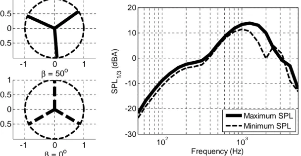
To gain a little more understanding on the increase of amplitude modulation strength when considering ground reflection and atmospheric absorption, a spectrum of amplitude modulation strength is plotted in Figure 17 for > = 1000N, in crosswind direction. It shows large frequency variations when ground reflection and atmospheric absorption are taken into account, while the free field spectrum is quite smooth. If we focus on the third octave band 2000vw, by looking at the spectra of the blade positions that produce maximum and minimum SPL in Figure 18, the
10 20 30 40 30 210 60 240 90 270 120 300 150 330 180 0 Free field
With G.R and A.A
2 4 6 30 210 60 240 90 270 120 300 150 330 180 0 Free field
8
cause of the 10 dB amplitude modulation peak is seen to be the ground interference dip at this frequency. It is necessary to notice that for different frequencies, the blade positions for maximum and minimum SPL are not necessary the same, thus the overall amplitude modulation strength is not simply the logarithm summation of the spectrum in Figure 17.
Figure 17. Spectrum of amplitude modulation strength. o p\\\q crosswind direction.
102 103 0 2 4 6 8 10 Frequency (Hz) A M s tr e n g th i n 1 /3 o c ta v e b a n d Free field
With ground ref. and atm. abs.
(a) P \^, down wind direction (b) P xr^
(c) P y\^, crosswind direction (d) P p\r^
Figure 16. Amplitude modulation strength with respect to source - receiver distance for P \^, xr^, y\^ z{| p\r^
0 200 400 600 800 1000 0 0.2 0.4 0.6 0.8 1 Distance (m) S tr e n g th o f A M ( d B A ) Free field With G.R and A.A
0 200 400 600 800 1000 0 0.2 0.4 0.6 0.8 1 Distance (m) S tr e n g th o f A M ( d B A ) Free field With G.R and A.A
0 200 400 600 800 1000 1.5 2 2.5 3 3.5 4 4.5 Distance (m) S tr e n g th o f A M ( d B A ) Free field With G.R and A.A
0 200 400 600 800 1000 5 5.5 6 6.5 7 7.5 8 Distance (m) S tr e n g th o f A M ( d B A ) Free field With G.R and A.A
9
Figure 18. Spectra of two 2 blade positions where the maximum and minimum SPL level are observed for the third octave band centred at } [\\\~•. o p\\\q, crosswind direction. Upper left: blade position where the maximum SPL is produced; Lower left: blade position where the minimum SPL is produced.
4.3 Accuracy of point source assumption for wind turbine noise
Wind turbine noise is an extended noise source, given the rotor diameter can be as large as 100 meters. But if the receiver is far enough, wind turbine noise may be modelled by a point source, and the calculation will be greatly simplified. The narrowband spectra of SPL for extended source and point source calculations are compared in Figure 19 for various source - receiver distance in downwind direction. From the figure we can see clearly that at R = 100m, the 2 spectra have similar level, but for point source, there are many interference dips. On the other hand the extended source spectrum is quite smooth, as already noticed by [Heutschi, 2014]. This is because the geometrical positions of the source and receiver are unique for a point source, while for the extended source, the distance between receiver and each segment are different. Thus the interference dips for each source (segment) - receiver distance occur at different frequencies using the extended source, as previously shown in figure 4(a). As a result, the overall SPL is smoothed out by the compensations. At a larger distance, for example, R = 1000m, the 2 spectra almost overlap for frequency less than 1kHz, and the first interference dips appear at the same frequency. This is because when the receiver is far, the distance differences between source (segment) - receiver are small, so even for an extended source, the first interference dip occurs at almost the same frequency, see figure 4(b). However at higher frequencies, there are still some interference dips for point source spectrum that are not observed for extended source. Similar results are observed for other directions.
-1 0 1 -0.5 0 0.5 β = 50o -1 0 1 -0.5 0 0.5 1 β = 0o 102 103 -30 -20 -10 0 10 20 Frequency (Hz) S P L 1 /3 ( d B A ) Maximum SPL Minimum SPL
10
(a) R = 100m (b) R = 200m
(c) R = 500m (d) R = 1000m
Figure 19. Narrow band SPL for point source and extended source at different source - receiver distance in downwind direction. Solid lines: extended source; dash lines: point source.
The overall SPL for extended source and point source with respect to distance in the downwind and crosswind direction are shown in Figure 20. From where we can see that there are no significant discrepancies, we can say that point source is a good simplification for overall immission level prediction. However, in Figure 21, it shows that the point source calculations over estimate the amplitude modulation strength in all the tested ground azimuthal directions. Close to crosswind direction, for τ 90X and 105X, the increases are significant.
(a) (b)
Figure 20. Overall SPL (immission level) with respect to distance in (a) downwind direction, (b) crosswind direction.
102 103 -10 -5 0 5 10 15 20 Frequency (Hz) S P L (d B A ) 102 103 -20 -15 -10 -5 0 5 10 15 Frequency (Hz) S P L (d B A ) 102 103 -35 -30 -25 -20 -15 -10 -5 0 5 Frequency (Hz) S P L (d B A ) 102 103 -60 -50 -40 -30 -20 -10 0 Frequency (Hz) S P L (d B A ) 200 400 600 800 1000 20 25 30 35 40 45 50
Distance to the source (m)
O v e ra ll S P L (d B A ) Extended source Point source 200 400 600 800 1000 15 20 25 30 35 40 45
Distance to the source (m)
O v e ra ll S P L (d B A ) Extended source Point source
11
(a) P \^, down wind direction (b) P xr^
(c) P y\^, crosswind direction (d) P p\r^
Figure 21. Amplitude modulation strength for extend source and point source calculation at different ground azimuthal angles.
5. Conclusions
Amiet's analytical model for trailing edge noise is able to predict noise emission from a wind turbine. The immission level is reduced at large distance mainly due to atmospheric absorption. Ground reflection modifies the shape of SPL spectrum. The amplitude modulation strength is increased when considering a grassland with atmospheric absorption. The point source assumption for wind turbine noise is good for predicting the overall immission level, but it overestimates the amplitude modulation strength, and cannot account for the frequency dependence of ground effects. A more accurate propagation model based on parabolic equation method [Cotte, et al., 2007 ] will be used in the future to take into account the effects of atmospheric turbulence and wind.
0 200 400 600 800 1000
0 0.5 1 1.5
Distance to the source (m)
S tr e n g th o f A M ( d B A ) Extended source Point source 0 200 400 600 800 1000 0 0.5 1 1.5
Distance to the source (m)
S tr e n g th o f A M ( d B A ) Extended source Point source 0 200 400 600 800 1000 2 2.5 3 3.5 4 4.5 5 5.5
Distance to the source (m)
S tr e n g th o f A M ( d B A ) Extended source Point source 0 200 400 600 800 1000 5 5.5 6 6.5 7 7.5 8 8.5
Distance to the source (m)
S tr e n g th o f A M ( d B A ) Extended source Point source
12
References
Amiet R.K (1975) Acoustic radiation from an airfoil in a turbulent stream, Journal of Sound and vibration 41(4), 407-420
Amiet R.K (1976) Noise due to turbulent flow past a trailing edge, Journal of Sound and Vibration 47(3), 387-393
Brooks T.F, Pope D.S and Marcolini M.A (1989) Airfoil self-noise and prediction, NASA reference publication 1218
Cotté B. and Blanc-Benon P (2007) Estimates of the relevant turbulent scales for acoustic
propagation in an upward refracting atmosphere. Acta Acustica United with Acustica, Vol.93.
Corcos G.M (1963) Resolution of pressure in turbulence, J. Acoust. Soc. Am. Vol.35, no.2 Creech A, Fruh W.G and Maguire A.E (2014) Simulations of an offshore wind farm using large
eddy simulation and a torque-controlled actuator disc model.
Chessell C.I (1977) Propagation of noise along a finite impedance boundary. J Acoust. Soc. Am. Vol. 62, No.4
Leloudas G (2006) Optimization of wind turbines with respect to noise, Master thesis DTU Heutschi K (2014) Auralization of Wind Turbine Noise: Propagation Filtering and Vegetation
Noise Synthesis, ACTA Acustica united with Acustica Vol. 100, 13-24
Oerlemans S, Schepers J.G (2009) Prediction of wind turbine noise and validation against
wexperiment, International Journal of Aeroacoustics, pp. 555-584.
Roger M and Moreau S (2005) Back-scattering correction and further extensions of Amiet's
trailing-edge noise model. Part 1: theory, Journal of Sound and Vibration, 286, 447-506
Rozenberg Y (2007) Modélisation analytique du bruit aérodynamique à large bande des
machines tournantes: utilisation de calculs moyennés de mécanique des fluides. PhD thesis,
L'école centrale de Lyon.
Rozenberg Y, Robert G, Moreau S (2012) Wall-pressure spectral model including the adverse
pressure gradient effects, AIAA Journal 50(10)
Samomons E.M (2001) Computational atmospheric acoustics. Kluwer Academic Publishers. Schlinker R.H and Amiet R.K (1981) Helicopter Rotor Trailing Edge Noise, NASA Contractor Report 3470.