Mesoscale circulations over complex terrain in the Valencia coastal region, Spain – Part 1: Simulation of diurnal circulation regimes

HAL Id: hal-00328496

https://hal.archives-ouvertes.fr/hal-00328496

Submitted on 16 Apr 2007

HAL is a multi-disciplinary open access

archive for the deposit and dissemination of

sci-entific research documents, whether they are

pub-lished or not. The documents may come from

teaching and research institutions in France or

abroad, or from public or private research centers.

L’archive ouverte pluridisciplinaire HAL, est

destinée au dépôt et à la diffusion de documents

scientifiques de niveau recherche, publiés ou non,

émanant des établissements d’enseignement et de

recherche français ou étrangers, des laboratoires

publics ou privés.

Valencia coastal region, Spain – Part 1: Simulation of

diurnal circulation regimes

G. Pérez-Landa, P. Ciais, M. J. Sanz, B. Gioli, F. Miglietta, J. L. Palau, G.

Gangoiti, M. M. Millán

To cite this version:

G. Pérez-Landa, P. Ciais, M. J. Sanz, B. Gioli, F. Miglietta, et al.. Mesoscale circulations over

complex terrain in the Valencia coastal region, Spain – Part 1: Simulation of diurnal circulation

regimes. Atmospheric Chemistry and Physics, European Geosciences Union, 2007, 7 (7), pp.1849.

�10.5194/acp-7-1835-2007�. �hal-00328496�

© Author(s) 2007. This work is licensed under a Creative Commons License.

Chemistry

and Physics

Mesoscale circulations over complex terrain in the Valencia coastal

region, Spain – Part 1: Simulation of diurnal circulation regimes

1_{Fundaci´on CEAM. Parque Tecnol´ogico, c/o Charles R. Darwin 14, 46980 Paterna (Valencia), Spain}

2_{Laboratoire des Sciences du Climat et de l’Environnement, UMR Commissariat `a l’Energie Atomique/CNRS 1572,}

Gif-sur-Yvette, France

3_{IBIMET-CNR, Instituto di Biometeorologia, Consiglio Nazionale delle Ricerche, Firenze, Italy}

4_{Escuela T´ecnica Superior de Ingenieros Industriales de Bilbao, Universidad del Pa´ıs Vasco/Euskal Herriko Unibertsitatea,}

Bilbao, Spain

Received: 22 December 2005 – Published in Atmos. Chem. Phys. Discuss.: 11 April 2006 Revised: 8 January 2007 – Accepted: 19 March 2007 – Published: 16 April 2007

Abstract. We collected ground-based and aircraft vertical

profile measurements of meteorological parameters during a 2-week intensive campaign over the Valencia basin, in order to understand how mesoscale circulations develop over com-plex terrain and affect the atmospheric transport of tracers. A high-resolution version of the RAMS model was run to sim-ulate the campaign and characterize the diurnal patterns of the flow regime: night-time katabatic drainage, morning sea-breeze development and its subsequent coupling with moun-tain up-slopes, and evening flow-veering under larger-scale interactions. An application of this mesoscale model to the transport of CO2is given in a companion paper. A careful

evaluation of the model performances against diverse me-teorological observations is carried out. Despite the com-plexity of the processes interacting with each other, and the uncertainties on modeled soil moisture boundary conditions and turbulence parameterizations, we show that it is possi-ble to simulate faithfully the contrasted flow regimes during the course of one day, especially the inland progression and organization of the sea breeze. This gives confidence with re-spect to future applicability of mesoscale models to establish a reliable link between surface sources of tracers and their atmospheric concentration signals over complex terrain.

1 Introduction

More than 75% of the Earth’s population live near the sea (Michener at al., 1997), with many coastal cities being

sur-Correspondence to: G. P´erez-Landa

(gorkapl@confluencia.biz)

rounded by hills or mountains. In coastal regions with com-plex terrain, the various atmospheric gases and aerosols emit-ted at the surface will be transporemit-ted by mesoscale circula-tions and injected into the atmosphere with very specific pat-terns. These patterns are not resolved in coarse-scale global transport models, and thus require further study to under-stand atmospheric transport processes at small scales. Solar heating frequently creates thermally induced mesoscale cir-culations that develop under clear sky conditions, with strong diurnal variations, and with patterns and intensities that de-pend on the regional surface energy budget and orography. The formation of pollution layers has been related to these mesoscale circulations, in particular to the interaction be-tween the sea breeze and mountain circulations. This process has been observed at Athens (Lalas et al., 1987), Los Ange-les (Lu and Turco, 1994), British Columbia, (McKendry et al., 1997), Tokyo (Chang et al., 1989), and over the Northern (Mill´an et al., 1984) and Eastern (Mill´an et al., 1992) coasts of Spain.

The Western Mediterranean Basin is surrounded by high mountains and during summer clear-sky conditions prevail. In total, 42 million people live in urban areas on the West-ern Mediterranean coast (Attane and Courbage, 2004). For-mer campaigns have shown that mesoscale processes domi-nate the meteorological regimes in this region (Mill´an et al., 1997). Regional circulations are diurnal and become self-organized from cells of a few tenths of a kilometer in their early development stages, up to circulations extending to the whole basin (hundreds of kilometers) later in the evening (Gangoiti et al., 2001). The presence of stacked layers of pollutants has been attributed to the mesoscale recirculation of airmasses in the Mediterranean basin (Mill´an et al., 1997).

Fig. 1. (a) Domain configuration and orography of the RAMS model showing the four nested domains with increasing horizon-tal resolution. The largest domain (GRID 1) has a grid length of 40.5 km, and the smallest (GRID 4) is of 1.5 km. (b) Character-istics of the smallest-domain simulated meteorological fields are compared to the campaign measurements. Black lines show the orography every 200 m. Grey-scaled colours show the different land cover types (see legend). The location of the meteorological stations (black circles), eddy-covariance flux towers (open squares), air-borne horizontal transect (black arrow) and vertical profiles (stars) can be seen.

Joint use of mesoscale models and Lagrangian particle dis-persion models was found useful in the description of trans-port patterns in this region (Gangoiti et al., 2001; P´erez-Landa et al., 2002).

The goal of this paper is to quantify and understand the at-mospheric transport processes acting on scales ranging from 1 to 100 km in the Western Mediterranean Region. To meet

this goal, an intensive measurement campaign was carried out during the summer of 2001 in the Valencia region, a coastal basin with complex terrain located on the East coast of Spain. The campaign was part of the European project RECAB (Regional Assessment and Modelling of the Carbon Balance in Europe). Airborne vertical profiles and ground based continuous measurements of meteorological variables were collected at different locations (Gioli et al., 2004). We used a high-resolution mesoscale model to interpret these measurements in terms of atmospheric transport processes. The following sections describe the typical summertime mesoscale transport processes in the Western Mediterranean area (Sect. 2), the campaign (Sect. 3) and, the model simula-tions (Sect. 4). The model results are evaluated against ob-servations (Sect. 5) and analyzed in the context of air masses recirculation and breeze effects (Sect. 6). A quantitative esti-mation of the model performances is made in Sect. 7. Carbon dioxide fluxes and concentrations were also measured during the campaign. In a follow-up paper (P´erez-Landa et al., 2007, this issue) we analyze the mesoscale transport of CO2using

the same atmospheric mesoscale model.

2 Relevant features at regional and local scales

The terrain of the Western Mediterranean Basin (WMB) ex-erts a strong influence on its weather regimes by generat-ing local and regional mesoscale circulations on diurnal time scales (Mill´an et al., 1997, 2002; Gangoiti et al., 2001). The main orographic features are illustrated in Fig. 1a. In sum-mer, sea breezes combine with up-slope winds to transport wet air inland, where it can be injected at the front of the combined breeze into a return flow at typical heights of 2– 3 km (Mill´an et al., 1997). During the day, the resulting generalized convergence of winds at ground level along the coast is compensated by an increased subsidence over the sea (Mill´an et al., 1997). During the night, these processes relax and gravity flows dominate along the coastal valleys, advect-ing inland air near the surface towards the sea (Mill´an et al., 1992). These processes create a marked diurnal cycle of the wind direction and pressure. They also enable a recircula-tion of air masses with a periodicity of a few days, as shown by tracer experiment results (Mill´an et al., 1992). Such mesoscale circulation cells involving vertical re-circulations and/or oscillations are also observed in the Central Mediter-ranean (Georgiadis et al., 1994; Orciari et al., 1998) and the Eastern Mediterranean basins (Kallos et al., 1998; Ziomas et al., 1998). Around the WMB mesoscale circulations can develop coherently at a scale that may encompass the whole basin (Mill´an et al., 1997; Gangoiti et al., 2001). This makes it necessary to consider mesoscale circulations around the WMB as a whole, in order to properly quantify and under-stand the transport patterns within a smaller region, here the Valencia basin.

Table 1. Flights carried out on 2 July.

Time Interval (UTC)

Type Coordinates Height

(m) 06:23–06:30 Profile 39.36 N; 0.35 W 15–800 07:40–07:45 Profile 39.37 N; 0.35 W 15–800 11:47–11:51 Profile 39.37 N; 0.36 W 15–800 13:03–13:08 Profile 39.36 N; 0.36 W 15–800 06:31–06:41 Hz. Transect 39.38 N; 0.36 W–39.21 N; 0.27 W 50 06:43–06:53 Hz. Transect 39.21 N; 0.27 W–39.38 N; 0.36 W 50 06:54–07:04 Hz. Transect 39.39 N; 0.35 W–39.21 N; 0.27 W 50 07:05–07:15 Hz. Transect 39.21 N; 0.27 W–39.38 N; 0.36 W 25 07:16–07:26 Hz. Transect 39.38 N; 0.35 W–39.21 N; 0.27 W 25 07:27–07:38 Hz. Transect 39.21 N; 0.27 W–39.39 N; 0.36 W 25 11:54–12:04 Hz. Transect 39.39 N; 0.36 W–39.20 N 0.27 W 50 12:05–12:15 Hz. Transect 39.21 N; 0.27 W–39.38 N 0.35 W 50 12:16–12:26 Hz. Transect 39.39 N; 0.36 W–39.21 N 0.27 W 50 12:27–12:37 Hz. Transect 39.21 N; 0.27 W–39.38 N; 0.38 W 25 12:39–12:49 Hz. Transect 39.39 N; 0.35 W–39.21 N; 0.27 W 25 12:52–13:02 Hz. Transect 39.21 N; 0.27 W–39.39 N; 0.34 W 25

The Valencia region is located on the East coast of the Iberian Peninsula. At the confluence of the Turia (North) and Jucar (South) river valleys, the region presents a coastal plain extending up to 50 km inland (Fig. 1b), surrounded by mountain ranges with an average elevation of 1000 m. The combination of fertile soils, proximity to the sea, mild tem-peratures and flat topography enables the large-scale culti-vation of irrigated tree-crops (mainly citrus) and paddy rice along the coast. The city of Valencia, located at the mouth of the Turia river (Fig. 1b), contains 1.4 M people, including conurbations, and has no heavy industry.

3 Airborne and ground-based measurements during the campaign

We focus here on the campaign episode of 1–2 July 2001, during which many vertical aircraft profiles were collected near the coastline, specifically over rice fields (Fig. 1a). The weather conditions for this episode show a high pressure sys-tem centered over the Netherlands and a typical decrease in sea level pressure towards the East in the Mediterranean re-gion (Fig. 2). There is a local pressure minimum over the center of the Iberian Peninsula at 12:00 UTC, where the tem-perature is locally warm at that time. Under such a typical summer weather pattern, mesoscale circulations are expected to develop in the Valencia basin.

The airborne measurements made on 2 July consist of ver-tical profiles and horizontal transects collected at selected in-tervals, using a Sky Arrow ERA light-weight aircraft (Ta-ble 1). Vertical profiles were taken between 15 m and 800 m above the rice fields. Eddy covariance flux measurements

were performed along each horizontal transect (Fig. 1b). The aircraft measured sensible and latent heat fluxes, tempera-ture, relative humidity and wind, and CO2 concentrations

and fluxes (the latter analyzed in a companion paper). These measurements are described by Gioli et al. (2004).

Airborne vertical profiles are collocated with ground-based eddy covariance flux measurements. Eddy-covariance, fluxes of CO2, H2O and energy were measured on top of two

towers (Fig. 1b). The first tower (12 m), called El Saler (SA), is permanently located over a Pine-dominated maquia forest. The second tower (2 m), called Rice (RI), was set up during the campaign over a rice field. Eddy covariance fluxes of sen-sible and latent heat (and CO2fluxes) are calculated at 30 min

time steps from ultrasonic anemometer wind, H2O and

tem-perature sensors 10 Hz data, following the guidelines of the Euroflux methodology (Aubinet et al., 2000). The measure-ments of wind speed and direction, temperature and relative humidity made on top of each flux tower were used to evalu-ate the results of the RAMS model (Sect. 5). Additional mea-surements come from five meteorological stations within the Valencia basin: Villar (VI) and X´ativa (XA) located inland, and Altura (AL), Port (PO) and Carraixet (CA), located in the North.

4 Mesoscale simulation: Model setup, initial and boundary conditions

The Regional Atmospheric Modeling System (RAMS; Pielke et al., 1992) in its version 4.3.0 was used to simulate selected days of the RECAB campaign. The RAMS model was applied to four domains of decreasing size at increasing

Fig. 2. Temperature (◦C) at 1000 hPa and Sea Level Pressure (hPa) fields from the AVN global model at 12:00 UTC on 2 July.

spatial resolution (Fig. 1a). A series of two-way interac-tive nested domains were configured at decreasing horizon-tal grid spacing of 40.5, 13.5, 4.5 and 1.5 km, respectively (Fig. 1a). The vertical discretization uses 45 levels with a 30 m spacing near the surface increasing gradually up to 1000 m near the model top at 17 000 m, and with 15 levels in the lower 1000 m. Our version of RAMS includes the Mel-lor and Yamada (1982) level 2.5 turbulence parameterization, a full-column two-stream single-band radiation scheme that accounts for clouds to calculate short-wave and long-wave radiation (Chen and Cotton, 1983), and a Kuo-modified pa-rameterization of sub-grid scale convection processes in the coarse domain (Molinari, 1985). The cloud and precipita-tion microphysics scheme from Walko et al. (1995) was ap-plied in all the domains. The LEAF-2 soil-vegetation surface scheme was used to calculate sensible and latent heat fluxes exchanged with the atmosphere, using prognostic equations for soil moisture and temperature (Walko et al., 2000).

Atmospheric boundary and initial conditions are derived from the analysis of the NCEP Aviation (AVN) run of the Global Spectral Model (Caplan et al., 1997), available ev-ery 6 h at ≈100 km resolution globally. A Four-Dimensional Data Assimilation (FDDA) technique is used to define the forcing at the lateral boundaries of the outermost eight grid cells of the largest domain. Surface boundary conditions also include land cover information. We use here the USGS land cover (Anderson et al., 1976) modified to include detailed land use information from CORINE (CEC, 1995) over the Iberian Peninsula, and from PELCOM (Mucher et al., 2000) over the rest of Europe. The various land cover types are re-classified into the 30 distinct LEAF-2 vegetation classes with an original resolution of 0.0083◦ (Baklanov et al., 2004). Over the ocean, we prescribe SST values at 0.5◦ resolu-tion by means of direct processing of NOAA-AVHRR raw satellite data during the days of the campaign following the

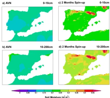
Fig. 3. Soil moisture for the 1st of July at 00:00 GMT: interpo-lated from the (a) 0–10 cm and (b) 10–200 layers of the AVN global model into RAMS domain 2; output of the 2 months spin up simu-lation over RAMS domain 2, vertically averaged (c) between 0 and 10 cm and (d) between 10 and 200 cm.

scheme by Badenas et al. (1997). In areas where processed data was not available (some peripheral areas located out-side GRID 2) data from weekly means global data (Reynolds, 1994) were used.

Soil-moisture plays a central role in controlling the devel-opment of mesoscale circulations, via its influence on the surface energy budget (Ookouchi et al., 1984; Lanicci et al., 1987; Jacobson 1999). Soil moisture is usually estimated in global models by using atmospheric variables as forcing data (Mahfouf, 1991). This procedure provides soil mois-ture gridded fields, which are otherwise impossible to obtain from direct observations. When soil moisture and tempera-ture from the AVN fields were used to initialize RAMS, how-ever, the simulated meteorological fields showed important differences against the measurements. The simulation was too dry (Table 2) and the morning vertical profiles of temper-ature during the morning were poorly captured (not shown). We thus initialized soil moisture and soil temperature dur-ing the campaign by runndur-ing RAMS coupled to LEAF-2 over the two largest domains (Fig. 1a) for two months pre-ceding the campaign, guided by a smooth data assimilation (FDDA) of the AVN fields. For simplicity, we prescribed LEAF-2 with a homogeneous soil texture of the clay-loam type. The soil column at each grid point is subdivided into 11 layers down to a depth of 2 m. The soil moisture was initialized with a uniform profile at a value of 0.38 m3/m3. The initial soil temperature profile is obtained by subtract-ing from the surface air temperature a value of 2.3◦C in the top soil, which linearly decreases down to a decrease of 1◦C

Fig. 4. Measured (continuous line) and simulated (discontinuous line) time series on 1 and 2 July 2001 in VI, XA and SA (see Fig. 1b). On the left: temperature (black) and q (grey). On the right: wind speed (grey) and wind direction (black). When the observed or simulated wind speed was less or equal to 0.5 ms−1, the wind direction was not drawn.

in the bottom soil. The soil variables obtained in RAMS for 1 July 2001 were compared to the AVN global analy-sis data. Soil temperatures were similar in both simulations, except for those regions where differences in model orog-raphy are important (not shown). Soil moisture from AVN was drier than in RAMS for the 0–10 cm layer, and for 10– 200 cm (Fig. 3). The RAMS results show their highest

mois-ture values in mountainous regions, probably due to the ef-fect of convective precipitation which the global AVN model could not resolve. Other differences in AVN vs. RAMS soil moisture fields must also be attributed to their different land surface schemes, which may induce different soil moisture dynamic ranges (see e.g., Koster and Milly, 1997).

Fig. 5. Scatter plot of virtual potential temperature vs. specific humidity hourly data at weather stations XA (red), VI (green) and SA (blue) observed (a) and modeled (b), for the daytime period of 06:00 to 18:00 UTC on 1 July (−1) and 2 July (−2).

Fig. 6. Observed (closed circles) and modeled (open circles) net radiation (black), sensible (red) and latent (blue) heat fluxes at SA surface station during 1 and 2 July 2001.

The use of a 2-month model spin-up to initialize our high-resolution simulation could be disputed, when compared with other more complex schemes employed in mesoscale models (e.g. Smith et al. 1994). However, initialized in this way, RAMS showed good skills in simulating wind and tem-perature fields during the campaign (Sect. 5 and P´erez-Landa et al., this issue).

5 Results: modeled and observed meteorological quan-tities

5.1 Model comparison with surface weather stations We focus here on time series from three stations shown in Fig. 1b, SA (El Saler, coastal), VI (Villar, inland in the Jucar river valley) and XA (X`ativa, inland in the Turia river valley). The two inland stations show a larger diurnal temperature cycle (15◦C) than the coastal station (8◦C), as seen in Fig. 4. The model captures quite well the diurnal temperature range at each station (see Sect. 6), as well as the gradient between the coastal station SA and the inland ones XA and VI. The warming trend observed at all three sites between 1 and 2 July, reaching up +5◦C in one day at XA, is well reproduced. However, there is a noticeable under-prediction of the SA diurnal temperature range, by up to 3◦C, with overly high minimum and overly low maximum values (Fig. 4e).

The air specific humidity shows a rather complex diurnal variation, different between the three stations and between 1 July and 2 July (Fig. 4). The observed humidity is on aver-age higher near the coast at SA, although the first day shows a dry spell in the morning. The XA station experiences a daytime drying which intensifies on 2 July, whereas the VI station has an opposite trend. Generally, the model is too wet compared to the observations at all three sites (Fig. 4), but it does reproduce the observed trend towards increasing humidity between 1 July and 2 July.

In the hourly wind speed and direction data shown in Fig. 4, we can observe a strong diurnal oscillation, character-ized by the daytime development of the sea-breeze advecting air from sea to land at a speed of up to 6 m s−1, followed by night time surface drainage winds oriented from land to sea. Thermal circulations develop during the day, stabiliz-ing a flow pattern advectstabiliz-ing air from sea to land. The wind blows inland from the East, but it is occasionally variable and

Fig. 7. (a) Early morning horizontal wind vectors at 50 m above ground. Thick black arrows: observed winds during the airborne transects at 06:50 UTC on 2 July. Thin grey arrows: modeled winds at the same time. Grey regions correspond to the same land cover types as in Fig. 1. (b) Same fields but for midday conditions, at 12:10 UTC. Note that corresponding wind scales are drawn at the top right of each panel.

its direction also varies between sites. At SA, winds blow-ing from the East were observed on 1 July, but they were seen to come from the North-East on the evening of 2 July (Fig. 4e). In XA, the winds blowed initially from the North-East, changed to the North-West by the evening of 1 July and to the South-West by the evening of 2 July. Gravity-driven drainage circulations develop during the night. The drainage winds follow the main axis of the valleys (Fig. 4 and Fig. 1b). Nocturnal winds blowing from the South-West along the Ju-car valley (Fig. 4d) were observed at XA. At VI, calm con-ditions within a stable stratified surface layer prevailed, with no representative wind direction. At SA near the coast, the wind blew from the South-West during the night of 2 July, and from the North-West during the night of 3 July. This sta-tion is located at the confluence of the Jucar and Turia valleys (Fig. 1b) so that the main nocturnal wind direction depends on which of the two drainage flows prevails.

It is very encouraging to see that the mesoscale model is able to capture quite realistically both the timing and the in-tensity of breezes and drainage winds (Fig. 4). At VI, the modeled wind speed and direction match the data during the day, except for the change in the evening of 2 July (Fig. 4). At XA, the model predicts a change in wind direction from

North-East to East by mid-day on 2 July, whereas the data show a variable wind direction. A second change in wind direction by the evening of 2 July is simulated, with winds from the North, while the observed winds are from the South-West. At SA, on the coast, the daytime sea breeze develop-ment is well-reproduced, especially for 2 July (Fig. 4). More discrepancies with the station data are observed during the night under stable conditions. At VI, the modeled drainage wind speed is overestimated by 1.5 m s−1, probably due to the presence of a ground inversion not resolved in the model, while at XA and SA the modeled winds are occasionally in the wrong direction.

The link between the mesoscale circulations and the ther-modynamic cycle can be analyzed with the help of conserved variable plots (Betts and Ball, 1995). Figure 5 shows the heating of airmasses observed during the early morning and, in general, coupled to drying processes. A sharp decrease in heating and an increase in specific humidity can then be observed in the six cycles analyzed. The moistening occurs with the set-up of the mesoscale circulations which advects humidity inland until the end of the daytime cycle. The only exceptions are XA and SA on the second day, which show a second stage of drying and heating processes. This could

Fig. 8. Experimental (left) and modeled (right) vertical profiles of horizontal winds over the rice paddy fields at the aircraft campaign location (marked with P in Fig. 1b) at different times on 2 July.

indicate some entrainment of dry and warm air from a layer aloft in the mixing layer.

The model results represented in Fig. 5 show important differences when compared with observations. The model presents moister values and less variability during the diur-nal cycle than measurements show (see also above). The model captures the moistening due to advection in SA, al-though it cannot see the strong heating and drying measured on the first day. This could be due to the early development of the simulated breeze circulation at SA compared to obser-vations (Fig. 4f). The model does not solve clearly the role advection plays in moistening the airmass at the inland sta-tions, although the presence of moister air before the arrival of the breeze could have decreased this effect. It is clear that the drying processes during the early stages of the cycle are very different from those observed, which could be due to the effect of our simple soil moisture initialization scheme. The model shows less variability than the aircraft data, sug-gesting that the spatial gradients in specific humidity are too small. The second stage of the drying and heating processes observed at XA and SA stations is not captured by the model. This could be due to the limitations of the PBL schemes sim-ulating the effect of the entrainment processes.

Figure 6 shows good agreement between simulated and observed net radiation and heat and moisture fluxes at SA. However, the singular location of this site as well as the het-erogeneous character of the region limits the representativity of this result. Thus, as our previous analysis on moisture suggests, more bias in the fluxes is expected throughout the domain.

5.2 Comparison between model and aircraft measurements

The horizontal winds measured at 50 m above ground during the aircraft transects are shown in Fig. 7. During the early morning (Fig. 7a), the drainage winds flow towards the sea. In the northern basin (Turia), the wind speed is low and the wind comes from the North-West, while in the southern basin (Jucar), the wind turns to the West and increases in speed. At the confluence of the Jucar and Turia valleys, the wind ac-quires a different direction and speed. There is good agree-ment between model and data, except for an underestimation of the drainage winds in the southern basin (Fig. 7a). In con-trast with the complex early-morning drainage wind fields (driven by orography and gravity), the mid-day wind field is more uniform, with a South-East origin and higher speeds than in the morning near the coast. This daytime breeze flow is nicely reproduced by RAMS (Fig. 7b).

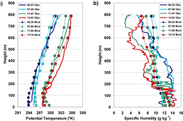
Figure 8 shows the wind vertical profiles measured on 2 July. The early morning data (06:23 UTC) indicate that the drainage winds are confined below ≈200 m. The next morn-ing profile (07:40 UTC) shows a transition period between drainage and sea breeze regimes, with low speeds at every altitude. Later in the day, the sea breeze develops and blows from the South-East at a speed of 5 m s−1 by 11:47 UTC, increasing up to 7 m s−1by 13:03 UTC. This breeze cell re-mains confined below 400 m throughout the day.

The changing shapes of the wind profiles are well captured by the model (Fig. 8). At 06:30 UTC, however the model underestimates the drainage wind intensity in the lowermost layers, while aloft there is overestimation. At 07:50 UTC, the model reproduces the drop in wind speed at the transition between drainage and breeze. At 11:50 UTC and 13:10 UTC, the model captures well the persistent breeze regime (see also Fig. 10), including the wind shear above ≈400 m.

Vertical profiles of potential temperature show the transi-tion between the drainage and breeze regimes (Fig. 9). Heat-ing occurs in the lower 200 m because of convective mixHeat-ing, and between 200 and 800 m because of the sinking of air in the compensatory subsidence capping the sea breeze (Mil-lan et al, 1997). The model reproduces the observed tem-perature profiles and rate of change well, suggesting that the mesoscale dynamics of the basin (also governing the CO2

dispersion) is realistic. Nevertheless, some discrepancies with the data can still be found in the lowest levels. The model cannot solve for the inversion present in the 06:37 profile near the ground, and at 11:50 UTC and 13:10 UTC while observed profiles are slightly stable, the model shows unstable profiles in the lowest 100 m. Both features could have a significant impact in the simulation of the atmospheric transport of any tracer. Additionally, the model is too wet in altitude, a bias also seen at surface stations, and it does not resolve explicitly the fine scale structure of the humidity pro-files (Fig. 9), owing to its coarse resolution.

Fig. 9. Observed (Obs) and modeled (Mod) vertical profiles of potential temperature (left) and q (right) over the rice paddy fields at the aircraft campaign location (marked with P in Fig. 1b) at different times on 2 July.

6 Modeled 3-D circulation patterns

In this section, we use the model as a tool which helps to understand the 3-D character of the complex terrain circula-tions identified in the previous data analysis. Figure 10 shows the surface horizontal streamlines and pressure fields during the course of 2 July. During the night, the drainage winds follow the direction of each valley (Fig. 10a). Vertical cross-sections show the thickness and extension of this drainage flow, which penetrates over the sea (Fig. 11a). After dawn, at 08:00 UTC, heating of the slopes oriented toward the sun allows the development of up-slope winds, while in some ar-eas close to the coast, nocturnal drainage persists (Fig. 10b). The gray lines in Fig. 10b show that vertical injection occurs at some well-defined convergence zones. In these conver-gence zones, positive vertical transport and upward advec-tion of TKE occur (see, for instance, at longitude −0.87 W in Fig. 11b). At the same time, there is a divergence zone at around −0.63 W, where vertical winds become negative in the lower 200 m and sinking of TKE is modeled (Fig. 11b). Higher than 400 m above the sea, the wind coming from the East is connected to the up-valley injection. The return flow can be observed above 1200 m. A similar divergence center was modeled in the southern Jucar valley, 38.95 N, −0.48 W, surrounded by convergence lines (Fig. 10b). The horizontal gradient of the Sea Level Pressure is small at this stage of the morning. This circulation consists of a complex pattern of horizontal and vertical winds, and the scales of the processes are related to the size of each valley.

At 11:00 UTC, the valley breezes have merged into a com-bined breeze extending from the sea (where horizontal winds are diverging) to a convergence line over the mountain range parallel to the coast (Figs. 10c and 11c). The vertical in-jection at this time of the day is stronger than it was ear-lier, reaching above 2000 m in height (Fig. 11c). The breeze cell stays confined to the first 400 m (Fig. 8), but it connects the coast with the mountain convergence and its return aloft. There is a continuous Sea Level Pressure decrease of 1–2 hPa within 60 km from the coast to the interior. The cross-section parallel to the coast (Fig. 11d) shows that the compensatory subsidence above the center of the valley limits the vertical mixing to the lower 300 m of the atmosphere.

At 15:00 UTC, the wind veers to the South-East over the sea, while inland the mountain convergence lines move per-pendicular to the coast (Fig. 10d). The negative pressure gradient between the valleys and the coast has further in-creased. Three hours later, at 18:00 UTC, while the wind direction over the sea continues to be from the South-East, the wind inland has changed to North-East in the southern basin and to South-East in the northern basin (Fig. 10e). The development of this circulation partly compensates for the negative pressure gradient between the coast and the valleys. At 21:00 UTC, the cooling of the surface starts to organize drainage winds towards the sea, while part of the flow reflects previous processes (Fig. 10f). The spatial variability of the pressure decreases, except in the higher north-east valleys.

Fig. 10. Horizontal streamlines and Sea Level Pressure simulations near the surface (at ≈15 m) at different intervals on 2 July: (a) at 06:00, (b) at 08:00 UTC, (c) at 11:00 UTC, (d) at 15:00 UTC, (e) at 18:00 UTC, and (f) at 21:00. The thick grey solid lines represent convergence lines of the horizontal wind. The black dotted lines indicate the location of the cross-sections drawn in Fig. 11. Closed circles represent the location of ground stations (Fig. 1b).

Fig. 11. Vertical cross-sections of simulated TKE (m2s−2) and wind (m s−1). Contour lines represent TKE and vectors represent the wind component projected in the direction of the section and with the vertical wind multiplied by 10. Each plot corresponds to the cross-sections drawn in Fig. 10 at constant latitude at the respective times, except for case (d) which represents a cross-section at constant longitude at 11:00 according to Fig. 10c. Note the different wind scaling in (b).

7 Quantitative estimates of the model performances

The ability of the RAMS model to reproduce mesoscale cir-culations over the complex terrain of the Valencia region serves a further, quantitative assessment. Table 2 gives a de-tailed statistical comparison between modeled and observed temperatures, specific humidities and winds. The meteoro-logical stations are grouped into a coastal group (PO, CA, SA, RI) and an inland group (AL, XA, VI). Hourly outputs of the model were spatially interpolated to the location of each station and compared to the data. We calculated the Mean Error (ME) and the Root Mean Square Error (RMSE)

for temperature and humidity. For winds, we calculated the RMSE of the Vector Wind Difference (see Stauffer and Sea-man 1990 and Table 2 caption), which takes into account both wind speed and direction errors, an important advan-tage in the presence of wind reversals. We also calculated the wind speed Index Of Agreement (IOA), which measures the degree to which a model’s prediction is free of error (Will-mott, 1981; a value of 0 means complete disagreement and a value of 1, perfect agreement).

Table 2. Model skills against surface observations. The seven surface stations are grouped by location into Coastal (PO, CA, SA and RI) and Inland (AL, VI and XA). N represents the number of observations included in the calculation of Mean Error, Root Mean Square Error, Index of Agreement and Vector Wind Difference for the respective variables. P represents the simulated value and Poobservation, while Mo

is the average observed wind speed for N values in the corresponding formulas: ME=_N1 N P i=1 (P − Po) IOA=1− N (RMSE) 2 N P i=1 (|P −Mo|+|Po−Mo|)2 VWD =p(u − uo)2+(v − vo)2 RMSE = s 1 N N P i=1 (P −Po)2

1–2 July 2001 Wind vector (ms−1) Temp. (◦C) q (g kg−1)

ME RMSE IOA VWD N ME RMSE N ME RMSE N

AVN Soil Cond.: All 0.62 1.61 0.79 2.29 300 0.18 2.28 300 −2.7 4.1 215 2 months spin-up:

All Stations All 0.36 1.54 0.79 2.18 300 0.04 1.49 300 0.33 3.53 215 Day 0.52 1.43 0.84 2.28 195 −0.15 1.48 195 0.72 3.58 140 Night 0.07 1.72 0.61 1.99 105 0.38 1.51 105 −0.39 3.44 75 Coastal Stations All 0.04 1.47 0.78 2.04 171 −0.03 1.43 171 −2.68 3.90 86 Day 0.36 1.21 0.86 2.11 111 −0.08 1.31 111 −2.29 3.83 56 Night −0.56 1.86 0.63 1.93 60 0.06 1.63 60 −3.41 3.96 30 Inland Stations All 0.79 1.63 0.80 2.36 129 0.13 1.56 129 2.34 2.97 129

Day 0.73 1.69 0.84 2.51 84 −0.24 1.67 84 2.72 3.18 84 Night 0.92 1.51 0.59 2.07 45 0.81 1.34 45 1.62 2.52 45

7.1 Temperature and humidity

The temperature RMSE for all stations is 1.49◦_{C, with a ME}

of 0.04◦C (i.e., no bias). The model performances for tem-perature are very good, if one compares the small value of the model-data misfit (Table 2) with either the large diurnal cycle amplitude of 15◦C (Fig. 4) or the coast minus inland temperature difference of 4◦C. When only the coastal sta-tions are considered, the model shows no bias (ME=0.03◦C) and performs equally well for daytime as for night time. For inland stations, the model has a slight negative bias dur-ing the day (ME=−0.24◦C) and a slight positive one dur-ing the night (ME=0.81◦C). This overestimate of the diurnal temperature cycle does not degrade the model-data compar-ison, the RMSE values for the inland stations being simi-lar to those of the coastal sites. For specific humidity, the value of the ME for all stations is small (0.33 g kg−1_),

in-dicating a slight wet bias in the model. The model simu-lates specific humidity less well than it does temperature, as illustrated by an RMSE value of 3.5 g kg−1 (see also Fig. 4). One can further see from Table 2 that the model is too dry near the coast (ME=−2.7 g kg−1)and too wet in-land (ME=2.4 g kg−1). The dry bias at the coastal stations is more pronounced during the night, while the wet bias at the inland stations is higher during the day.

7.2 Winds

The model shows a slight positive bias for winds (ME=0.36 m s−1). Averaged for all the weather stations, we simulated typical nocturnal wind values of 1 m s−1, and day-time values of 6 m s−1, giving a diurnal amplitude 5 m s−1 (see Fig. 4). The simulated wind has an RMSE of 1.54 m s−1, which suggests good model performances, given the ampli-tude of the signal. The wind speed IOA is 0.79, which is good, given the complexity of the flow and the fact that the seven stations represent contrasted wind regimes. The mod-eled wind speed at the coastal stations is accurate (ME=0.04), but at the inland stations it is too high (ME=0.79 m s−1). In both cases, the mean bias remains lower than the RMSE. At inland sites, the wind speed RMSE is similar between day and night (Table 2). Considering that nocturnal winds are four times weaker than diurnal ones, this suggests worse model skills inland at night. At coastal sites, a positive bias is found during the day (ME=+0.36 m s−1), and a negative one during the night (ME=−0.56). The model performances are again worse during the night. Overall, during the night, the model is too windy inland and not windy enough on the coast.

For all stations, the RMSE of Vector Wind Difference (RMSE-VWD) varies between 1.2 and 2.5 m s−1, with a peak at 4 m s−1 (Fig. 12). It is clear from Fig. 12 that

the model simulates the wind vector worse for inland sites (VWD=7 m s−1_{)than for coastal sites. For the coastal sites,}

maximum RMSE-VWD occurs at 20:00 UTC and proba-bly corresponds to the period of transition from the evening breeze to the nocturnal drainage. Except for evening transi-tions, the VWD values remain between 1 and 3 m s−1 with no differences between coastal and inland locations. Mini-mum values of 1 m s−1are observed when the wind speed is weaker, e.g., during the night of 1 July.

8 Concluding remarks

By combining measurements and models, we were able to identify three characteristic mesoscale circulation regimes over the Valencia basin: 1) a nocturnal drainage flow with katabatic winds channeled by the valleys, 2) a combined breeze regime during which the sea breeze merges with con-vective uplift over the mountain ranges followed by a sub-siding flow over the sea, and 3) an evening regime where a large inland pressure minimum can interact with the com-bined breeze and change the flow pattern. Such regimes commonly develop in the Valencia region under summertime conditions.

Soil moisture and soil temperature in the RAMS model were initialized by a 2-months spin-up. This simple initial-ization procedure improved the model results for the atmo-spheric fields as compared to prescribing global AVN soil moisture fields (Table 2). Yet, the initial soil moisture fields seem to cause a wet bias of the atmospheric model inland, and a dry bias near the coast (Figs. 4 and 5). Despite this, the model statistical skills and the model evaluation in terms of processes controlling temperature and wind diurnal vari-ations, are both in good agreement with the data. In fact, our statistical scores were comparable to those of other simi-lar simulation studies (Seaman and Michelson, 2000; Hanna and Yang 2001; Zhong and Fast 2003) and the model’s abil-ity to solve processes was similar to other studies in complex terrain (Zhong and Fast, 2003; De Wekker et al., 2005).

One of the most interesting processes captured here is the combined breeze circulation cell, in particular its subsidence branch towards the sea which increases the temperature in-version and confines mixing to the lowermost 200 m despite solar heating rates higher than 700 Wm−2. A second impor-tant process solved by the model is the evening circulation generated when solar warming diminishes to compensate the spatial preassure gradient formed after heat distribution dur-ing the daytime mesoscale processes development (Fig. 10e). Finally, the main processes and spatial flow patterns dur-ing the nocturnal regime are captured with high accuracy, although the comparison with station observations (Fig. 4), and consequently the statistical evaluation (Table 2), show some discrepancies. It seems that the model results are hor-izontally more homogeneous than reality, and that the stable boundary layer parameterization of RAMS does not

repro-Fig. 12. Time series of VWD averaged for the seven surface stations (Solid) and grouped by location as Coast: PO, CA, SA and RI (dots) and Inland: AL, VI and XA (dashed).

duce the high spatial variability of the wind in the area. Addi-tionally, the early morning temperature profile solved by the model shows some vertical mixing while the observed pro-file remains stable (Fig. 9). Both results could indicate that during the nocturnal regime the model produces too much mixing through interactions with orography and thus homog-enizes the flow in excess. Although more experimental data would be desirable to confirm this hypothesis, our results are consistent with those of Zhong and Fast (2003), who, when evaluating different mesoscale models in complex ter-rain, found stronger vertical mixing and diffusion than the observed values during the nocturnal regime.

It is well known that landscape and terrain heterogeneities induce spatially varying surface turbulent fluxes, resulting in heterogeneous boundary layers (Pielke, 2002). Our model study area combines the difficulties of land-sea contrasts, mountainous terrain and larger-scale mesoscale circulations. The measurements available during the campaign allowed us to characterize the breeze development in the lower atmo-sphere near the coast, although vertical profiles to a higher altitude and further inland would also have been very use-ful. It is very encouraging to note that, despite the inherent complexity of the system studied and the limitations from unknown initial soil moisture distribution, the RAMS model could reproduce faithfully the main mesoscale flow patterns. However, it is important to keep in mind that turbulence pa-rameterizations of mesoscale models are derived from the-ories and data for horizontally homogeneous steady-state boundary layers (Pielke, 2002). Thus, it is likely that the simulated turbulence fields (usually provided for dispersion models) could have been conditioned by this limitation. New data over complex terrain could be useful to test mesoscale models beyond their range of normal applicability, with the aim of eventually improving them.

Acknowledgements. This work has been partially supported by the

projects RECAB (EVK2-CT-1999-00034) and CARBOEUROPE-IP (GOCE-CT-2003-505572), funded by the European Com-mission. The authors wish to thank all those who worked hard to collect the data in the field. We are grateful to D. Sotil for his support with the graphics. Also thanks to J. A. Alloza and J. V. Chord´a for reclassifying CORINE and PELCOM physiogra-phy data into RAMS land use categories. J. Scheiding’s corrections of the English text are appreciated. We are also grateful to three anonymous referees for their constructive comments which signifi-cantly improved the paper. NCEP and ECMWF are acknowledged for providing meteorological analysis and reanalysis data. The CEAM foundation is supported by the Generalitat Valenciana and BANCAIXA.

Edited by: W. E. Asher

References

Anderson, J. R., Hardy, E. E., Roach, J. T., and Witmer, R. E.: A land use and land cover classification system for use with re-mote sensor data, U.S. Geological Survey Professional Paper 964, Government Printing Office, Washington D.C., Available on-line http://landcover.usgs.gov/pdf/anderson.pdf, 1976. Attane, I. and Courbage, Y.: Demography in the Mediterranean

re-gion. Plan Bleu. Paris, Economica, available on-line http://www. planbleu.org/publications/demo uk part1.pdf, 2004 .

Aubinet, M., Grelle, A., Ibrom,A., Rannik, U., Moncrieff, J., Fo-ken, T., Kowalski, A. S., Martin, P. H., Berbigier, P., Bernhofer, C., Clement, R., Elbers, J., Granier, A., Grunwald, T., Morgen-stern, K., Pilegaard, K., Rebmann, C., Snijders, W., Valentini, R., and Vesala, T.: Estimates of the annual net carbon and water exchange of European forests: the EUROFLUX methodology, Adv. Ecol. Res., 30, 113–175, 2000.

Badenas, C., Caselles, V., Estrela, M. J., and Marchuet R.: Some improvements on the processes to obtain accurate maps of sea surface temperature from AVHRR raw data transmitted in real time. Part. 1. HRPT images, Int. J. Rem. Sens., 18, 1743–1767, 1997.

Baklanov, A., Batchvarova, E., Calmet, I., Clappier, A., Chord´a, J. V., Di´eguez, J. J., Dupont, S., Fay, B., Fragkou, E., Hamdi, R., Kitwiroon, N., Leroyer, S., Long, N., Mahura, A., Mestayer, P., Nielsen, N. W., Palau, J. L., P´erez-Landa, G., Penelon, T., Rantam¨aki, M., Schayes G., and Sokhi, R. S.: Improved pa-rameterisations of urban atmospheric sublayer and urban physio-graphic data classification, D4.1, 4.2 and 4.5 FUMAPEX Report, edited by: Baklanov, A. and Mestayer, P., DMI, Denmark, DMI Scientific Report: #04-05, ISBN nr. 87-7478-506-0., 2004. Betts, A. K. and Ball J. H.: The FIFE surface diurnal cycle climate,

J. Geophys. Res., 100(D12), 25 679–25 694, 1995.

Caplan, P., Derber, J., Gemmill, W., Hong, S. Y., Pan, H. L., and Parish, D.: Changes to the NCEP operational medium-range forecast model analysis/forecast system, Weat. Forecasting, 12, 581–594, 1997.

CEC (Commission of the European Communities): CORINE Land cover, Guide Technique, Brussels, Available on-line, http:// reports.eea.eu.int/COR0-landcover/en, 1995.

Chang, Y. S., Carmichael, G. R., Kurita, H., and Ueda, H.: The transport and formation of photochemical oxidants in Central

Japan, Atmos. Environ., 23, 363–393, 1989.

Chen, C. and Cotton, W. R.: A one-dimensional simulation of the stratocumulus-capped mixed layer, Boundary-Layer Meteorol., 25, 289–321, 1983.

De Wekker, S. F. J., Steyn, D. G., Fast, J. D., Rotach, M. W., and Zhong, S.: The performance of RAMS in representing the con-vective boundary layer structure in a very steep valley, Environ. Fluid Mech., 5, 35–62, 2005.

Gangoiti, G., Mill´an, M. M., Salvador, R., and Mantilla, E.: Long-range transport and re-circulation of pollutants in the western Mediterranean, during the project Regional Cycles of Air Pol-lution in the West-Central Mediterranean Area, Atmos. Environ., 35, 6267–6276, 2001.

Georgiadis, T., Giovanelli, G., and Fortezza, F.: Vertical layering of photochemical ozone during land-sea breeze transport, Il Nuovo Cimento, 17, 371–375, 1994.

Gioli, B., Miglietta, F., De Martino, B., Hutjes, R. W. A., Dolman, H. A. J., Lindroth, A., Schumacher, M., Sanz, M. J., Manca, G., Peressotti, A., and Dumas, E. J.: Comparison between tower and aircraft-based eddy covariance fluxes in five European regions, Agric. For. Meteorol., 127, 1–16, 2004.

Hanna, S. R. and Yang, R.: Evaluations of mesoscale model simu-lations of near-surface winds, temperature gradients, and mixing depths, J. Appl. Meteorol., 40, 1095–1104, 2001.

Jacobson, M. Z.: Effects of soil moisture on temperatures, winds, and pollutant concentrations in Los Angeles, J. Appl. Meteorol., 38, 607–616, 1999.

Kallos, G., Kotroni, V., Lagouvardos, K., and Papadopoulos, A.: On the long-range transport of air pollutants from Europe to Africa, Geophys. Res. Lett., 25(5), 619–622, 1998.

Koster, R. D. and Milly, P. C. D.: The interplay between transpira-tion and runoff formulatranspira-tions in land surface schemes used with atmospheric models, J. Climate, 10(7), 1578–1591, 1997. Lalas, D. P., Tombrou-Tsella, M., Petrakis, M., Asimakopoulos,

D. N., and Helmis, C.: An experimental study of the horizon-tal and vertical distribution of ozone at Athens, Atmos. Environ., 21, 2681–2693, 1987.

Lanicci, J. M., Carlson, T. N., and Warner, T. T.: Sensitivity of the Great Plains severe-storm environment to soil-moisture distribu-tion, Mon. Wea. Rev., 115, 2660–2673, 1987.

Lu, R. and Turco, R. P.: Air pollutant transport in a coastal envi-ronment. Part I. Two-dimensional simulations of sea-breeze and mountain effects, J. Atmos. Sci., 51, 2285–2308, 1994. Mahfouf, J. F.: Analysis of Soil Moisture from Near-Surface

Pa-rameters: A Feasibility Study, J. Appl. Meteorol., 30, 1534– 1547, 1991.

McKendry, I. G., Steyn, D. G., Lundgren, J., Hoff, R. M., Strapp, W., Anlauf, K., Froude, F., Martin, J. B., Banta, R. M., and Olivier, L. D.: Elevated ozone layers and vertical downmixing over the Lower Fraser Valley, BC, Atmos. Environ., 31, 2135– 2146, 1997.

Mellor, G. L. and Yamada, T.: Development of a turbulence clo-sure model for geophysical fluid problems, Rev. Geophys. Space Phys., 20, 851–875, 1982.

Michener, W. K., Blood, E., R., Bildstein, K. L., Brinson, M. M., and Gardner, L. R.: Climate change, hurricanes and tropical storms, and rising sea level in coastal wetlands, Ecol. Appl., 7(3), 770–801, 1997.

Ureta, I.: A fumigation episode in an industrialized estuary: Bil-bao, November 1981, Atmos. Environ., 18, 563–572, 1984. Mill´an, M. M., Arti˜nano, B., Alonso, L., Castro, M.,

Fernandez-Patier, R., and Goberna, J.: Meso-Meteorological Cycles of Air Pollution in the Iberian Peninsula, (MECAPIP), Air Pollution Research Report 44, EUR No. 14834, European Commission DG XII/E-1, Rue de la Loi, 200, B-1040, Brussels, 1992.

Mill´an, M. M., Salvador, R., Mantilla, E., and Kallos, G.: Photoox-idants dynamics in the Mediterranean basin in summer: Results from European research projects, J. Geophys. Res., 102(D7), 8811–8823, 1997.

Molinari, J.: A general form of Kuo cumulus parameterisation, Mon. Wea. Rev., 113, 1411–1416, 1985.

Mucher, C. A., Steinnocher, K. T., Kressler, F. P., and Heunks, C.: Land cover characterisation and change detection for environ-mental monitoring of pan-Europe, Int. J. Remote Sens., 21(6–7), 1159–1181, 2000.

Ookouchi, Y., Segal, M., Kessler, R. C., and Pielke, R. A.: Evalua-tion of soil moisture effects on the generaEvalua-tion and modificaEvalua-tion of mesoscale circulations, Mon. Wea. Rev., 112, 2281–2292, 1984. Orciari, R., Georgiadis, T., Fortezza, F., Alberti,, L., Leoncini, G., Venieri, L., Gnani, V., Montanari, T., and Rambelli, E.: Vertical evolution of photochemical ozone over greater Ravenna, Annali di Chimica, 88, 403–411, 1998.

P´erez-Landa, G., Palau , J. L., Mantilla, E., and Mill´an, M. M.: A study of the dispersion of an elevated plume on complex terrain under summer conditions, paper presented at 15th Symposium on Boundary Layers and Turbulence, American Meteorological Society, Wageningen, The Netherlands, 346–349, 2002. P´erez-Landa, G., Ciais, P., Gangoiti, G., Palau, J. L., Carrara, A.,

Gioli, B., Miglietta, F., Schumacher, M., Mill´an, M., and Sanz, M. J.: Mesoscale circulations over complex terrain in the Valen-cia coastal region, Spain – Part 2: Modeling CO2transport us-ing idealized surface fluxes, Atmos. Chem. Phys., 7, 1851–1868, 2007.

Pielke, R. A., Cotton, W. R., Walco, R. L., Tremback, C. J., Lyons, W. A., Grasso, L. D., Nicholls, M. E., Moran, M. D., Wesley, D. A., Lee, T. J., and Copeland, J. H.: A comprehensive meteo-rological modelling system RAMS, Meteorol. Atmos. Phys., 49, 69–91, 1992.

Pielke Sr., R. A.: Mesoscale meteorological modeling. 2nd Edition, Academic Press, San Diego, CA, 676 pp, 2002.

Reynolds, R. W. and Smith, T. M.: Improved global sea surface temperature analyses using optimum interpolation, J. Climate, 7, 929–948, 1994.

Seaman, N. L. and Michelson, S. A.: Mesoscale meteorological structure of a high-ozone episode during the 1995 NARSTO-Northeast study, J. Appl. Meteorol., 39(3), 384–398, 2000. Smith, C. B., Lakhtakia, M. N., Capehart, W. J., and Carlson, T.

N.: Initialization of soil-water content in regional-scale atmo-spheric prediction models, Bull. Amer. Meteorol. Soc., 75, 585– 593, 1994.

Stauffer, D. R. and Seaman, N. L.: Use of Four-Dimensional Data Assimilation in a limited-area mesoscale model. Part I: Experi-ments with Synoptic-Scale Data, Mon. Wea. Rev., 6, 1250–1277, 1990.

Walko, R. L., Band, L. E., Baron, J., Kittel, T. G. F., Lammers, R., Lee, T. J., Ojima, D., Pielke Sr. R. A., Taylor, C., Tague, C., Tremback, C. J., and Vidale, P. J.: Coupled atmospheric-biophysics-hydrology models for environmental modeling, J. Appl. Meteorol., 39, 931–944, 2000.

Walko, R. L., Cotton, W. R., Meyers, M. P., and Harrington, J. Y.: New RAMS cloud microphysics parameterization. Part I: The single-moment scheme, Atmos. Res., 38, 29–62, 1995.

Willmott, C. J.: On the validation of models, Phys. Geog., 2, 184– 194, 1981.

Zhong, S. and Fast, J.: An evaluation of MM5, RAMS, and Meso ETA at sub-kilometer resolution using VTMX field campaign data in the Salt Lake Valley, Mon. Wea. Rev., 131, 1301–1322, 2003.

Ziomas, I. C., Gryning, S. E., Borstein, R. D. (Eds.): The Mediter-ranean campaign of photochemical tracers-transport and chem-ical evolution (MEDCAPHOT-TRACE): Athens, Greece 1994– 1995, Atmos. Environ., 32, 2043–2326, 1998.