HAL Id: hal-01185206
https://hal.inria.fr/hal-01185206
Submitted on 19 Aug 2015
HAL is a multi-disciplinary open access
archive for the deposit and dissemination of
sci-entific research documents, whether they are
pub-lished or not. The documents may come from
teaching and research institutions in France or
abroad, or from public or private research centers.
L’archive ouverte pluridisciplinaire HAL, est
destinée au dépôt et à la diffusion de documents
scientifiques de niveau recherche, publiés ou non,
émanant des établissements d’enseignement et de
recherche français ou étrangers, des laboratoires
publics ou privés.
Bootstrapped Permutation Test for Multiresponse
Inference on Brain Behavior Associations
Bernard Ng, Jean Baptiste Poline, Bertrand Thirion, Michael Greicius
To cite this version:
Bernard Ng, Jean Baptiste Poline, Bertrand Thirion, Michael Greicius. Bootstrapped Permutation
Test for Multiresponse Inference on Brain Behavior Associations. Information Processing in Medical
Imaging 2015, Sebastien Ourselin, University College London, UK; Daniel Alexander, University
Col-lege London, UK; Carl-Fredrik Westin, Harvard University, USA, Jun 2015, Sabhal Mor Ostaig, Isle
of Skye, United Kingdom. pp.12. �hal-01185206�
adfa, p. 1, 2011.
© Springer-Verlag Berlin Heidelberg 2011
Bootstrapped Permutation Test for Multiresponse
Inference on Brain Behavior Associations
Bernard Ng1,2, Jean Baptiste Poline2,3, Bertrand Thirion2, Michael Greicius1, and IMAGEN Consortium
1Functional Imaging in Neuropsychiatric Disorders Lab, Stanford University, United States 2Parietal team, Neurospin, INRIA Saclay, France
3Hellen Wills Neuroscience Institute, University of California Berkeley, United States
Abstract. Despite that diagnosis of neurological disorders commonly involves
a collection of behavioral assessments, most neuroimaging studies investigating the associations between brain and behavior largely analyze each behavioral measure in isolation. To jointly model multiple behavioral scores, sparse mul-tiresponse regression (SMR) is often used. However, directly applying SMR without statistically controlling for false positives could result in many spurious findings. For models, such as SMR, where the distribution of the model pa-rameters is unknown, permutation test and stability selection are typically used to control for false positives. In this paper, we present another technique for in-ferring statistically significant features from models with unknown parameter distribution. We refer to this technique as bootstrapped permutation test (BPT), which uses Studentized statistics to exploit the intuition that the variability in parameter estimates associated with relevant features would likely be higher with responses permuted. On synthetic data, we show that BPT provides higher sensitivity in identifying relevant features from the SMR model than permuta-tion test and stability selecpermuta-tion, while retaining strong control on the false posi-tive rate. We further apply BPT to study the associations between brain connec-tivity estimated from pseudo-rest fMRI data of 1139 fourteen year olds and be-havioral measures related to ADHD. Significant connections are found between brain networks known to be implicated in the behavioral tasks involved. More-over, we validate the identified connections by fitting a regression model on pseudo-rest data with only those connections and applying this model on resting state fMRI data of 337 left out subjects to predict their behavioral scores. The predicted scores are shown to significantly correlate with the actual scores of the subjects, hence verifying the behavioral relevance of the found connections.
Keywords: Bootstrapping, brain behavior associations, connectivity, fMRI,
multiresponse regression, permutation test, statistical inference
1
Introduction
Diagnosis of neurological disorders generally entails assessments of multiple behav-ioral domains. For instance, Attention Deficit Hyperactivity Disorder (ADHD) is
commonly diagnosed based on a collection of criteria related to inattention, hyperac-tivity, and impulsivity as specified in the Diagnostic and Statistical Manual of Mental Disorders (DSM). Thus, for most cases, it is the aggregate of multiple criteria that characterizes a neurological disorder. Past neuroimaging studies investigating brain behavior relationships typically analyze each behavioral measure independently [1]. One of the state-of-the-art approaches for jointly modeling multiple response varia-bles is to incorporate a group least absolute shrinkage and selection operator (LASSO) penalty into the regression model [2] to promote selection of features asso-ciated with all response variables. However, directly applying this sparse multi-response regression (SMR) technique and assuming that all features corresponding to nonzero regression coefficients are relevant could result in many spurious findings, since SMR alone does not control for false positives [3]. Another approach is to find linear combinations of features and responses that best correlate with each other using partial least square (PLS) or canonical correlation analysis (CCA), which can be cast as a reduced rank regression (RRR) problem [4]. In limited sample settings, especially when the number of features exceeds the number of samples, sparse variants of PLS, CCA, and RRR are often used [5], but these sparse variants in their raw forms suffer the same limitation as SMR in terms of false positives not being controlled.
The growing feature dimensionality of today’s problems warrants caution in con-trolling for false positives [6]. A number of techniques have been put forth for ad-dressing this critical concern in the context of sparse regression [7]. The key idea behind these techniques is to de-bias the sparse regression coefficient estimates, so that parametric inference can be applied to generate approximate p-values. How to de-bias the parameter estimates of SMR as well as sparse variants of PLS, CCA, and RRR is currently unclear. For models with unknown parameter distribution, a widely-used technique is permutation test (PT) [8], which is applicable to any statistics gen-erated from the model parameters since PT requires no assumptions on the underlying parameter distribution. Another flexible technique is stability selection (SS) [9], which operates under the rationale that if we subsample the data many times and per-form feature selection on each subsample using e.g. SMR, relevant features will likely be selected over a large proportion of subsamples, whereas irrelevant features will unlikely be repeatedly selected. Importantly, SS has a theoretical threshold that bounds the expected number of false positives. Also, SS eases the problem of regular-ization level selection in penalized models, such as SMR, in which only a range of regularization levels needs to be specified without having to choose a specific level. However, as we will show in Section 2.2 and 4, the choice of threshold and regulari-zation range has a major impact on the results.
Further complicating statistical inference on multi-feature models is the problem of multicollinearity [3]. In the face of correlated features, small perturbations to the data can result in erratic changes in the parameter estimates. In particular, sparse models with a LASSO penalty tends to arbitrarily select one feature from each correlated set [3]. One way to deal with this problem is to perturb the data e.g. by subsampling as employed in SS, and examine which features are consistently selected. Complement-ing this strategy is a technique called Randomized LASSO, which involves deweighting a random subset of features for each subsample. This combined
tech-nique is shown to improve relevant feature identification over pure subsampling [9]. Another strategy is to cluster the features to moderate their correlations, which has the additional advantage of reducing the feature dimensionality [3].
In this paper, we present a technique that combines bootstrapping with permutation test for inferring significant features from models with unknown parameter distribu-tion. We refer to this technique as bootstrapped permutation test (BPT). BPT is origi-nally proposed for inferring significant features from classifier weights [10], but as discussed here and in the next section, BPT is in fact applicable to arbitrary models with a number of properties that makes it advantageous over PT and SS. Bootstrap-ping is traditionally used for assessing variability in model parameters. In BPT, the variability differences in parameter estimates with and without permutation are ex-ploited. The intuition is that parameter estimates of relevant features are presumably more variable when responses are permuted. Thus, dividing the parameter estimates with and without permutation by their respective standard deviation should magnify their magnitude differences. This intuition is incorporated by using Studentized statis-tics, as generated by taking the mean of bootstrapped parameter estimates and divid-ing it by the standard deviation. The Studentized statistics is known to be approxi-mately normally-distributed [11]. Thus, we can generate a null distribution by fitting a normal distribution to Studentized statistics derived from the permuted responses, thereby enabling parametric inference, which is statistically more powerful than pure PT [12]. Also, BPT is more flexible than SS, since it can directly operate on parame-ter estimates from any models without the need for feature selection, which could be nontrivial for certain non-sparse models that do not possess an inherent feature selec-tion mechanism. In this work, we focus on the SMR model for drawing associaselec-tions between brain connectivity estimated from functional magnetic resonance imaging (fMRI) data and multiple behavioral measures related to attention deficit hyperactivi-ty disorder (ADHD). Functional connectivihyperactivi-ty is hyperactivi-typically estimated by computing the Pearson’s correlation between fMRI time series of brain region pairs, which are high-ly inter-related. To reduce the correlations between these connectivity features, we cluster them based on the network to which each brain region belongs, thereby ac-counting for the similarity between time series of brain regions within the same net-work. To compare BPT against PT and SS, we generate synthetic behavioral scores using network-level connectivity estimates derived from real fMRI data. We also apply these techniques on pseudo-rest fMRI data from 1139 fourteen year olds in identifying significant connections that are relevant to ADHD behavioral measures. The identified connections are validated on resting state fMRI data from 337 left out subjects by comparing their predicted and actual scores.
2
Methods
We first briefly review SMR (Section 2.1) and describe how stability selection (Sec-tion 2.2) can be incorporated to control for false positives. We then discuss the prop-erties of PT, and how BPT improves upon PT via the use of Studentized statistics as generated by bootstrapping (Sections 2.3).
2.1 Sparse Multiresponse Model
Let Y be a n×q matrix, where n is the number of samples, and q is the number of re-sponse variables. Further, let X be a n×d matrix, where d is the number of features. The standard way for assessing associations between Y and X is via regression:
2 2 Xβ Y β min , (1)
where β is the d×q regression coefficient matrix. The optimal β obtained by solving (1) is equivalent to regressing each column of Y on X independently. Thus, the rela-tions between columns of Y are ignored. To incorporate this information in estimating
β, one of the state-of-the-art approaches is to employ the SMR model [2]:
1 , 2 2 2 g minY Xβ β β , s.t. d i q j ij d i i g 1 1 2 2 1 :, 1 , 2 β β β (2)
where ||βg||2,1 is the group LASSO penalty and each row of β, denoted as βi,:,
corre-sponds to a feature. With elements of each βi,: taken as a group, only features
associ-ated with all q response variables would be selected with the corresponding βi,j ≠ 0 for
all j. To set λ, we search over 100 λ’s in [λmax, λmin], where λmax = maxj||X:,jTY||2 and
λmin = cλmax, c < 1. Optimal λ is defined as the one that minimizes the prediction error over 1000 subsamples with the data randomly split into 80% for model training and 20% for error evaluation. A fast solver of (2) is implemented in GLMNET [13].
2.2 Stability Selection
A problem with assuming features associated with nonzero βi,: in SMR are all relevant
is that this property is true only under very restricted conditions, which are largely violated in most real applications [3]. In particular, this guarantee on correct feature selection does not hold when features are highly correlated, which is often the case for real data [3]. With correlated features, perturbations to the data can result in drastic changes in the features that are selected. Based on this observation, an intuitive ap-proach to deal with correlated features is to perturb the data and declare features that are consistently selected over different perturbations as relevant, which is the basis of SS. We describe here SS in the case of SMR, but SS can generally be applied to any models that are equipped with a feature selection mechanism. Given X, Y, and [λmax, λmin], SS combined with Randomized LASSO proceeds as follows [9]:
1. Multiply each column of X by 0.5 or 1 selected at random. 2. Randomly subsample X and Y by half to generate Xs and Ys.
3. For each λ in [λmax, λmin], apply SMR to generate βs(λ). Let Ss(λ) be a d×1 vector with elements corresponding to selected features, i.e. nonzero βs(λ), set to 1.
4. Repeat steps 2 and 3 S times, e.g. with S = 1000.
5. Compute the proportion of subsamples, πi(λ), that each feature i is selected for
each λ in [λmax, λmin].
A πth that controls for the expected number of false positives, E(V), is given by [9]:
d V E 2 th 1 2 1 , (3)where V is the number of false positives and γ is the expected number of selected features, which can be approximated by: 1/S·∑s∑i(UλSis(λ)). Uλ denotes the union over
λ. We highlight two insights on (3) that have major implications on applying SS in
practice. First, (3) is a conservative bound on the family-wise error rate (FWER) =
P(V≥1), since E(V) = ∑v=1∞ P(V≥v) > P(V≥1). To control FWER at α = 0.05 with
mul-tiple comparison correction (MCC), i.e. P(V≥1) ≤ α/d, even for γ = 1, πth based on (3) is >1. Since πi(λ) ϵ [0,1], πth should be clipped at 1, but whether FWER is still con-trolled is unclear. Second, a key property of SS is that it does not require choosing a specific λ. However, for n/2 > d, a “small enough” λmin could lead to all features being selected in all subsamples, resulting in maxλπi(λ) = 1. Hence, all features would be
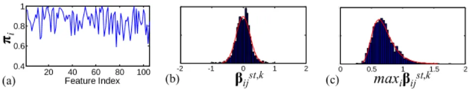
declared as significant. λ selection is thus translated into λmin selection, which warrants caution. An example from real data (Section 3.2) illustrating the impact of λmin and πth is shown in Fig. 1(a). Even with λmin set to 0.1, i.e. a λ range that would strongly en-courage sparsity, a πth of 0.9 (strictest πth in the suggested range of [0.6, 0.9] in [9]) declares >40% of the features as significant, i.e. fails to control for false positives.
Fig. 1. Behavior of SS and BPT on real data. (a) πi(λ) at λ = 0.1 (for SS). (b) Gaussian fit on
Studentized statistics (for BPT). (c) Gumbel fit on maxima of Studentized statistics (for BPT).
2.3 Bootstrapped Permutation Testing
For models with unknown parameter distribution, including those with no intrinsic feature selection mechanisms, PT is often used to perform statistical inference. PT involves permuting responses a large number of times (e.g. 10000 in this work) and relearning the model parameters for each permutation in generating null distributions of the parameters. Features with original parameter values greater than (or less than) a certain percentile of the null, e.g. >100·(1‒0.025/d)th percentile (or <100·(0.025/d)th percentile), are declared as significant. Equivalently, one can count the number of permutations with parameter values exceeding/below the original parameter values to generate approximate p-values. A key attribute of PT is that it does not impose any distributional assumptions on the parameters, but the cost of this flexibility is the need for a large number of permutations to ensure the resolution of the approximate p-values are fine enough for proper statistical testing, i.e. the smallest p-value attaina-ble from N permutation is 1/N. Also, if the underlying parameter distribution is known, the associated parametric test is statistically more powerful [12].
20 40 60 80 100 0.4 0.6 0.8 1 Feature Index πi (a) -2 -1 0 1 2 0 100 200 (b) βijst,k -2 -1.5 -1 -0.5 0 0 100 200 (c) maxiβijst,k
The central idea behind BPT is to generate Studentized statistics via bootstrapping to exploit how the variability of the parameter estimates associated with relevant fea-tures are likely higher with responses permuted. Similar to PT, BPT can be applied to any models. We describe here BPT in the context of SMR, which proceeds as follows.
Estimation of Studentized statistics, βijst:
1. Bootstrap X and Y with replacement for B = 1000 times, and denote the boot-strap samples as Xb and Yb.
2. Multiply each column of Xb by 0.5 or 1 selected at random.
3. Select the optimal λ for SMR by repeated random subsampling on X and Y, and apply SMR on Xb and Yb for each bootstrap b with this λ to estimate βb.
4. Compute Studentized statistics, βijst = 1/B·∑bβijb / std(βijb), where std(βijb) is the
standard deviation over bootstrap samples. Estimation of the null distribution of βijst:
5. Permute Y for N = 500 times.
6. For each permutation k, compute βijst,k with the same λ, samples, and feature
weighting used in each bootstrap b as in the non-permuted case.
7. p-value = 2·min(1‒Ф(βijst|1/N·∑kβijst,k, std(βijst,k)), Ф(βijst|1/N·∑kβijst,k, std(βijst,k))),
where Ф(·) = the cumulative distribution function of the normal distribution. To account for multiple comparisons, one can apply Bonferroni correction, but this technique tends to be too conservative [8]. A more sensitive technique is to use max-imum statistics [8], which entails finding the maxmax-imum βijst,k over i for each response
variable j and permutation k. Since βijst,k is approximately normally-distributed [11],
its maximum statistics should follow a Gumbel distribution. We can thus fit a Gumbel distribution to the maxima of βijst,k for each j and declare features associated with βijst
exceeding a certain percentile of the fitted Gumbel distribution as significant. Nega-tive βijst can be similarly tested with maximum replaced by minimum. An example
from real data (Section 3.2) illustrating a Gaussian and a Gumbel distribution fit to the empirical distribution of βijst,k and its maxima, respectively, for an exemplar feature
and response is shown in Fig. 1(b) and (c). Another sensitive MCC technique is false discovery rate (FDR) correction [8], which involves sorting the p-values in ascending order, and testing the lth p-value against l·α/d, e.g. α = 0.05.
We highlight here properties of BPT that make it advantageous over PT and SS. First, std(βijb) of relevant features are likely larger with responses permuted. By using
Studentized statistics, i.e. dividing the bootstrapped mean of βij by std(βijb), the
mag-nitude differences in βij between the permuted and non-permuted cases would be
magnified. Second, Studentized statistics approximately follows a normal distribution [11], hence justifying the use of parametric inference, which is more powerful than PT. It is worth noting that normal approximation on Studentized statistics is more accurate than on conventional mean [11], which provides another reason for dividing by the standard deviation. Lastly, in contrast to SS, BPT does not require a feature selection mechanism. Instead, BPT can directly operate on the parameter estimates, which additionally accounts for the magnitude of βij. Also, BPT facilitates greater
flexibility in the choice of statistical inference procedures, e.g. MCC with maximum statistics cannot be easily incorporated into SS.
3
Materials
3.1 Synthetic Data
To generate synthetic data, we used the network connectivity matrix, Xreal, estimated from pseudo-rest fMRI data (Section 3.2), which comprised 1139 subjects and 105 features. This way, the feature correlations present in the real data would be retained to enable method evaluation under more realistic settings. Two scenarios were con-sidered: n = 50 < d = 105 and n = 200 > d = 105. For each scenario, we generated 50
n×3 response matrices, Ysyn. Each Ysyn was created by randomly selecting n out of 1139 subjects and 10 out of 105 features taken as ground truth. Denoting the resulting
n×10 feature matrix as Xsyn, we generated Ysyn as Xsynβsyn + ε, where βsyn is a d×3 matrix with each element randomly drawn from a uniform distribution, U(0.01, 0.1), and ε corresponds to Gaussian noise. Each Ysyn and the corresponding n rows of Xreal (i.e. with all features kept, not Xsyn) constituted as one synthetic dataset.
3.2 Real Data
Neuroimaging and behavioral data from ~1,000 fourteen year olds were obtained from the IMAGEN database [14]. Details on data acquisition can be found in [14]. In this work, we focused on 3 behavioral measures of the Cambridge Neuropsychologi-cal Test Automated Battery (CANTAB) associated with ADHD [15]. SpecifiNeuropsychologi-cally, we examined the between error and strategy scores of the spatial working memory (SWM) task as well as the response accuracy score of the rapid visual information processing (RVP) task. For estimating connectivity, we used fMRI data acquired dur-ing a localizer task (140 volumes) as well as at rest (187 volumes) for model traindur-ing and validation, respectively. For the task fMRI data, slice timing correction, motion correction, and spatial normalization to MNI space were performed using SPM8. Motion artifacts, white matter and cerebrospinal fluid confounds, principal compo-nents of high variance voxels found using CompCor [16], and their shifted variants as well as task paradigm convolved with the canonical hemodynamic response and dis-crete cosine functions (for highpass filtering at 0.008 Hz) were regressed out from the task fMRI time series. The task regressors were included to decouple co-activation from connectivity in generating pseudo-rest data. The resting state fMRI data were similarly preprocessed except a bandpass filter with cutoff frequencies of 0.01Hz and 0.1Hz was used. Taking the intersection of subjects with all 3 behavioral scores and task fMRI data, while excluding those who also have resting state fMRI data to ensure that subjects for model training and validation are independent, 1139 subjects were available for model training. For validation, 337 subjects with all 3 behavioral scores and rest data were available. To estimate connectivity, we generated brain region time series by averaging the voxel time series within the 90 regions of interest (ROIs) of a publicly available functional atlas that span 14 large-scale networks [17]. The Pear-son’s correlation between ROI time series was taken as estimates of connectivity. Since time series of ROIs within the same network would be similar, the magnitude of their correlation with other ROIs would also be similar. To reduce the correlations
between these connectivity features, we computed the within and between network connectivity from the 90×90 Pearson’s correlation matrix. For estimating within net-work connectivity, we averaged the Pearson’s correlation values between all ROI pairs within each network, which resulted in 14 features. For estimating between work connectivity, we averaged the Pearson’s correlation values of all between net-work ROI connections for each netnet-work pair, which resulted in 91 features. Age, sex, scan site, and puberty development scores were regressed out from both the behavior-al scores and the network connectivity features (separately for the training and vbehavior-alida- valida-tion subjects), which were further demeaned and scaled by the standard deviavalida-tion.
4
Results and Discussion
On synthetic (Section 4.1) and real data (Section 4.2), we compared BPT at p < 0.05 with maximum statistics-based MCC and FDR correction against SMR with features associated with non-zero regression coefficients assumed significant, SS at p < 0.05/d with πth set based on (3) and πth = 0.75 (midpoint of suggested range of [0.6, 0.9] in [9], and PT at p < 0.05 with maximum statistics-based MCC and FDR correction. Central to applying SMR is the choice of λ. We thus examined results for λmin = 0.001, 0.01 and 0.1. Setting λmin to 0.1 produces a very narrow λ range that tends to generate overly-sparse β. This value of λmin was considered due to SS’s failure to control for false positives for smaller λmin in our real data experiments.
4.1 Synthetic Data
We evaluated the contrasted techniques by computing the average true positive rate (TPR) and average false positive rate (FPR) over the 50 synthetic datasets for each
n/d scenario. TPR was defined as the proportion of ground truth significant features
that were correctly identified, and FPR was defined as the proportion of ground truth non-significant features that were incorrectly found. Results for n/d = 50/105 and n/d = 200/105 are shown in Figs. 2 and 3. PT declared all features as non-significant, hence its results were not displayed. Also, λmin = 0.1 led to degraded performance for all techniques, which was likely due to the resulting λ range enforcing overly-sparse solutions. We thus focused our discussion on results for λmin = 0.001 and 0.01.
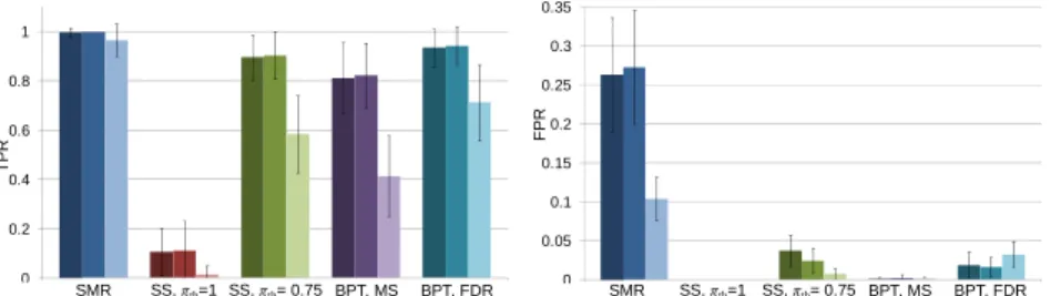
Fig. 2. Synthetic data results for n/d = 50/105 < 1. Each set of three bars (left to right)
corre-spond to λmin = 0.001, 0.01, and 0.1, respectively. MS = maximum statistics. 0 0.2 0.4 0.6 0.8 1 SMR SS, πth=1 SS, πth= 0.75 BPT, MS BPT, FDR TP R 0 0.05 0.1 0.15 0.2 0.25 0.3 0.35 SMR SS, πth=1 SS, πth= 0.75 BPT, MS BPT, FDR FP R
For n/d = 50/105, SMR achieved a TPR close to 1, but also included many false positives. Using SS with πth set based on (3) had FPR well controlled, but TPR was merely 0.1. Note that πth was >1 in all cases even without MCC, and was thus clipped at 1. By relaxing πth to 0.75, SS’s TPR increased to ~0.9, and FPR was <0.04, despite FPR control was not guaranteed. Using BPT with maximum statistics-based MCC, which exerts strong control over FPR, attained a TPR of ~0.8 with FPR being close to 0. Relaxing the control on FPR using FDR correction resulted in TPR of ~0.94 and FPR < 0.02, which is half the FPR of SS with πth = 0.75. Thus, for similar control on FPR, BPT provides higher sensitivity than SS. For n/d = 200/105, all contrasted tech-niques (except PT) achieved a TPR of ~1, but FPR was not well controlled with SMR and SS. In particular, SS with πth = 0.75 resulted in a FPR of 1 for λmin = 0.001due to all features being selected for small λ’s near λmin across all subsamples. Thus, declar-ing features as significant if πi(λ) ≥ πth for any λ could be erroneous for small λmin in
n > d settings. Also worth noting was the lack of sensitivity with PT, which clearly
demonstrates the enhanced sensitivity gained by using Studentized statistics in BPT. Nevertheless, PT with n = 1139 attained a TPR of ~1 and FPR close to 0.
Fig. 3. Synthetic data results for n/d = 200/105 > 1. Each set of three bars (left to right)
corre-spond to λmin = 0.001, 0.01, and 0.1, respectively. MS = maximum statistics.
4.2 Real Data
We applied the contrasted techniques to the pseudo-rest fMRI data of 1139 subjects to identify the significant network connections associated with ADHD behavioral measures. Since the ground truth is unknown, we validated the identified connections by first fitting a regression model (1) to the pseudo-rest data but with only the identi-fied connections retained. We then applied these models to the resting state fMRI data of 337 left out subjects to predict their behavioral scores. The Pearson’s correlation between the predicted and actual scores of these subjects was computed with signifi-cance declared at the nominal α level of 0.05.
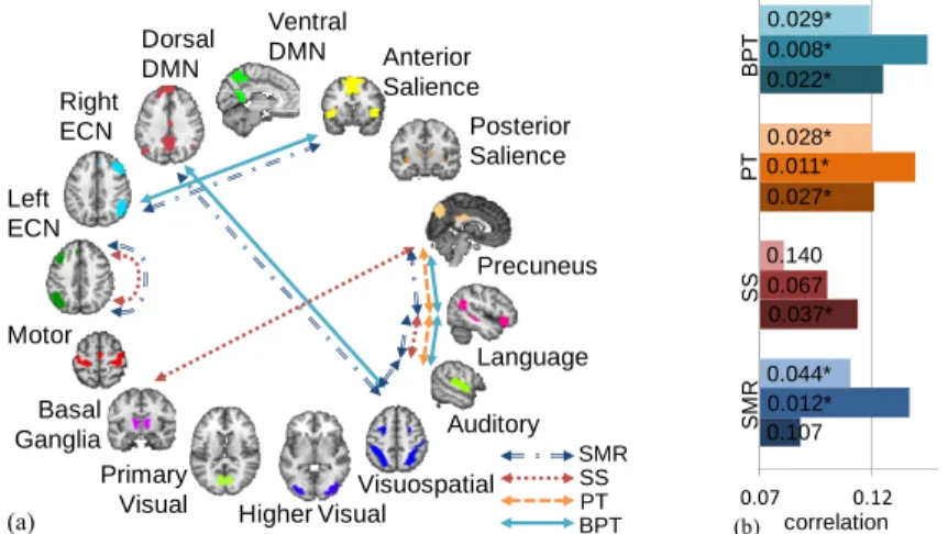
Using BPT with FDR correction, connections between the right executive control network (ECN) and the anterior salience network (ASN), the language network and the auditory network, the visuospatial network and the dorsal default mode network (DMN), as well as the precuneus and the language network were found to be signifi-cant (Fig. 3). These findings were consistent for λmin = 0.001 and 0.01. The Pearson’s correlation between the predicted and actual scores was significant for all three
be-0 0.2 0.4 0.6 0.8 1 SMR SS, πth=1 SS, πth= 0.75 BPT, MS BPT, FDR TP R 0 0.1 0.2 0.3 0.4 0.5 0.6 0.7 0.8 0.9 1 SMR SS, πth=1 SS, πth= 0.75 BPT, MS BPT, FDR FP R
havioral measures. The ECN comprises the dorsolateral prefrontal cortex (DLPFC) and the parietal lobe, which are involved with vigilance, selective and divided atten-tion, working memory, executive functions, and target selection [18]. Strongly con-nected to the DLPFC is the dorsal anterior cingulate cortex (part of the ASN), which plays a major role in target and error detection [18]. Hence, the finding of the connec-tion between the ECN and the ASN to be significant matches well with the cognitive processes required for the SWM and RVP tasks. Also, the visuospatial manipulation and memory demands involved with these tasks would explain the detection of the connection between the visuospatial network and the dorsal DMN. The detection of the connection between the precuneus and the language network might relate to the variability in the level of linguistic strategy employed by the subjects to process spa-tial relations [19]. Interestingly, although all subjects have subclinical ADHD scores, there is moderate variability in their values [20], which might explain the resemblance between the found networks and those affected by ADHD [18, 21, 22]. We note that BPT with the stricter maximum statistics-based MCC detected only the connection between the Precuneus and the language network.
SMR found connections between the visuospatial network and the language net-work as well as connections within the left ECN to be behaviorally relevant, in addi-tion to those found by BPT. These extra connecaddi-tions, although seem relevant, resulted in the Pearson’s correlation for the RVP task to fall below significance. As for SS, πth > 1 based on (3) for all λmin tested, even for E(V) < 0.05 instead of 0.05/d, i.e. no MCC. Setting λmin to 0.001 and 0.01 resulted in almost all network connections de-clared as significant for πth = 1. For λmin = 0.1, only one connection survived with πth = 1, and >1/3 of the connections declared significant with πth = 0.9 (Fig. 1(a)). To obtain sensible results, we used πth = 1 with λmin = 0.05, which declared the connections be-tween the language network and the auditory network, the primary visual network and the precuneus, as well as connections within the left ECN as significant. With these connections, only the Pearson’s correlation for the RVP task was significant. Using PT detected connections between the Precuneus and the language network as well as the language network and the auditory network, which constitutes a subset of the connections found by BPT, and the Pearson’s correlations obtained were similar.
We highlight here several notable observations. First, our results show that models built from pseudo-rest data can generalize to true rest data. This finding provides further support for the hypothesis that intrinsic brain activity is sustained during task performance [23]. The correlations between the predicted and actual scores, however, are rather small in absolute terms, which might limit practical applications. Second, SS is gaining popularity due to its generality and claimed robustness to regularization settings. Our results show that SS is actually sensitive to the choice of threshold and regularization range, especially for n > d. Thus, SS should be applied with caution. Third, applying BPT with 1/B·∑bβijb without diving by std(βijb) resulted in degraded
performance (similar to PT’s), which indicates that modeling differences in variability between the permuted and non-permuted cases is key to BPT’s superior sensitivity. Lastly, Studentized bootstrap conference intervals are known to have lower coverage errors than its empirically derived counterpart [24]. The observed improvements with BPT over PT could partly be attributed to this property of Studentized statistics.
Fig. 4. Real data results. λmin = 0.001, except SS where λmin = 0.05 used. (a) Significant network
connections found on pseudo-rest fMRI data. (b) Pearson’s correlation between predicted and actual scores with p-values noted. Each set of three bars (top to bottom) correspond to SWM strategy, SWM between errors, and RVP accuracy scores. *Significance declared at p < 0.05.
5
Conclusions
We presented BPT for statistical inference on models with unknown parameter distri-butions. Superior performance over PT and SS was shown on both synthetic and real data. The resemblance of the found networks with those implicated in ADHD sug-gests the associated network connections might be promising for ADHD classifica-tion, which currently has accuracy <70% with most neuroimaging-based classifiers.
Acknowledgements. Bernard Ng is supported by the Lucile Packard Foundation for
Children’s Health, Stanford NIH-NCATS-CTSA UL1 TR001085 and Child Health Research Institute of Stanford University. Jean Baptiste Poline is partly funded by the IMAGEN project (E.U. Community's FP6, LSHM-CT-2007-037286).
References
1. Seeley, W.W., Menon, V., Schatzberg, A.F., Keller, J., Glover, G.H., Kenna, H., Reiss, A.L., Greicius, M.D.: Dissociable Intrinsic Connectivity Networks for Salience Processing and Executive Control. J Neurosci. 27, 2349‒2356 (2007)
2. Simon, N., Friedman, J., Hastie, T.: A Blockwise Descent Algorithm for Group-penalized Multiresponse and Multinomial Regression. arXiv:1311.6529 (2013)
3. Varoquaux, G., Gramfort, A., Thirion, B.: Small-sample Brain Mapping: Sparse Recovery on Spatially Correlated Designs with Randomization and Clustering. Int. Conf. Machine Learning (2012)
4. De la Torre, F.: A Least-Squares Framework for Component Analysis. IEEE Trans. Patt. Ana. Mach. Intell. 34, 1041–1055 (2012)
Ventral DMN Dorsal DMN Right ECN Anterior Salience Posterior Salience Precuneus Language Auditory Basal Ganglia Primary
Visual Higher VisualVisuospatial Left ECN Motor SMR SS PT BPT (a) 0.07 0.12 1 correlation BP T PT SS SM R 0.029* 0.008* 0.022* 0.028* 0.011* 0.027* 0.140 0.067 0.037* 0.044* 0.012* 0.107 (b)
5. Le Floch, E., Guillemot, V., Frouin, V., Pinel, P., Lalanne, C., Trinchera, L., Tenenhaus, A., Moreno, A., Zilbovicius, M., Bourgeron, T., Dehaene, S., Thirion, B., Poline, J.B., Duchesnay, E.: Significant Correlation between a Set of Genetic Polymorphisms and a Functional Brain Network Revealed by Feature Selection and Sparse Partial Least Squares. NeuroImage 63, 11–24. (2012)
6. MacArthur, D.: Methods: Face up to False Positives. Nature 487, 427–428 (2012) 7. Javanmard, A., Montanari, A.: Confidence Intervals and Hypothesis Testing for
High-Dimensional Regression. arXiv:1306.3171 (2013)
8. Nichols, T., Hayasaka, S.: Controlling the Familywise Error Rate in Functional Neuroi-maging: a Comparative Review. Stat. Methods Med. Research 12, 419‒446 (2003) 9. Meinshausen, N., Bühlmann, P.: Stability Selection. J. Roy. Statist. Soc. Ser. B 72, 417–
473 (2010)
10. Ng, B., Dresler, M., Varoquaux, G., Poline, J.B., Greicius, M.D., Thirion, B.: Transport on Riemannian Manifold for Functional Connectivity-based Classification. In: Golland, P., Hata, N., Barillot, C., Hornegger, J., Howe, R. (eds.) MICCAI 2014. LNCS, vol. 8674, pp. 405–413. Springer, Heidelberg (2014)
11. Delaigle, A., Hall, P., Jin, J: Robustness and Accuracy of Methods for High Dimensional Data Analysis based on Student’s t-statistic. arXiv:1001.3886 (2010)
12. Tanizaki, H.: Power Comparison of Non-parametric Tests: Small-sample Properties from Monte Carlo Experiments. J. Applied Stat. 24, 603–632 (1997)
13. http://www.stanford.edu/~hastie/glmnet_matlab/
14. Schumann, G., et al.: The IMAGEN Study: Reinforcement-related Behaviour in Normal Brain Function and Psychopathology. Mol. Psychiatr. 15, 1128–1139 (2010)
15. Chamberlain, S.R., Robbins, T.W., Winder-Rhodes, S., Müller, U., Sahakian, B.J, Black-well, A.D., Barnett, J.H.: Translational Approaches to Frontostriatal Dysfunction in Atten-tion-Deficit/Hyperactivity Disorder Using a Computerized Neuropsychological Battery. Biol Psychiatry 69, 1192–1203 (2011)
16. Behzadi, Y., Restom, K., Liau, J., Liu, T.T.: A Component based Noise Correction Method (CompCor) for BOLD and Perfusion based fMRI. NeuroImage 37:90‒101(2007)
17. Shirer, W.R., Ryali, S., Rykhlevskaia, E., Menon, V., Greicius, M.D.: Decoding Subject-driven Cognitive States with Whole-brain Connectivity Patterns. Cereb. Cortex 22, 158−165 (2012)
18. Bush, G., Valera, E.M., Seidman, L.J.: Functional Neuroimaging of Attention-Deficit/Hyperactivity Disorder: A Review and Suggested Future Directions. Biol Psychia-try 57, 1273‒1284 (2005)
19. Wallentin, M., Weed, E., Østergaard, L., Mouridsen, K., Roepstorff, A.: Accessing the Mental Space-Spatial Working Memory Processes for Language and Vision Overlap in Precuneus. Hum. Brain Mapp. 29, 524‒532 (2008)
20. Whelan, R., et. al.: Adolescent Impulsivity Phenotypes Characterized by Distinct Brain Networks. Nat Neurosci. 15, 920‒925 (2012)
21. Westerberg, H., Hirvikoski, T., Forssberg, H., Klingberg, T.: Visuo-spatial Working Memory Span: A Sensitive Measure of Cognitive Deficits in Children with ADHD. Child Neuropsychol. 10, 155‒161 (2004)
22. Ghanizadeh, A.: Sensory Processing Problems in Children with ADHD, A Systematic Re-view. Psychiatry Investig. 8, 89‒94 (2011)
23. Fox, M.D., Raichle, M.E.: Spontaneous Fluctuations in Brain Activity Observed with Functional Magnetic Resonance Imaging. Nat. Rev. Neurosci. 8, 700–711 (2007)
24. Kuonen, D.: Studentized Bootstrap Confidence Intervals based on M-estimates. J. Applied Stats. 32, 443‒460 (2005)