HAL Id: halshs-01535172
https://halshs.archives-ouvertes.fr/halshs-01535172
Submitted on 8 Jun 2017
HAL is a multi-disciplinary open access archive for the deposit and dissemination of sci-entific research documents, whether they are pub-lished or not. The documents may come from teaching and research institutions in France or abroad, or from public or private research centers.
L’archive ouverte pluridisciplinaire HAL, est destinée au dépôt et à la diffusion de documents scientifiques de niveau recherche, publiés ou non, émanant des établissements d’enseignement et de recherche français ou étrangers, des laboratoires publics ou privés.
The value of time and expenditures of rural households
in Burkina Faso: a domestic production framework
François Gardes, Noël Thiombiano
To cite this version:
François Gardes, Noël Thiombiano. The value of time and expenditures of rural households in Burkina Faso: a domestic production framework. 2017. �halshs-01535172�
Documents de Travail du
Centre d’Economie de la Sorbonne
The value of time and expenditures of rural households in Burkina Faso: a domestic production framework
François GARDES, NoëlTHIOMBIANO
The value of time and expenditures of rural households in Burkina Faso: a domestic production framework
François Gardes, Paris School of Economics, University of Paris I Panthéon-Sorbonne, CES, France
Maison des Sciences Economiques, 106-112 Boulevard de l’Hôpital, 75640, Paris Cedex 13 ; tel. 01 44 07 83 14 ; 01 44 07 88 88
Noël Thiombiano, University of Ouaga II, CEDRES, Burkina Faso 03 BP 7210, Ouaga O3
Tel: (+226) 70 27 33 20 Email: thiombianonoel@yahoo.fr Abstract
We use a unique survey of rural households in Burkina Faso which contains both disaggregated households’ expenditures and time uses for nine domestic activities. This allows us to estimate the opportunity cost of time using a Beckerian model of domestic production based on a direct utility depending on activities which are home produced with market goods and time. Proxies for full prices of domestic activities allow to recover full income and full price elasticities as well as elasticities with respect to the monetary prices and time use costs. Finally, inequality is found to be smaller when measured by full income compared to inequality of households’ monetary incomes.
Keywords: domestic production, full income, full price, opportunity cost of time, price elasticity,
Burkina Faso.
JEL classification: C33, D13, J22
1. Introduction
Estimates of price elasticities on aggregate time series data are questionable both from a statistical and an economic standpoint. They often suffer from the co-linearity of prices changes and the insufficient change of relative prices. Price-elasticities estimates on macro time series data are therefore generally considered as not being robust to the specification of the demand system and to the estimation method. They also suffer from aggregation biases and lack of information, because the stationarity conditions cannot be verified for long term series. Moreover, they are not able to take care of various constraints binding the household choices, especially in African countries. We propose in this article to use a new approach to estimate price effects on micro cross-sectional data based on using full prices derived from a budget survey containing both households’ expenditures and time uses.
In addition to the precision obtained in the estimation over a large population, using individual level data allows us to differentiate the demand functions across different sub-population defined by age group, family structure or location, characteristics which may be
related to differences in preferences or economic constraints. It also gives rise to estimates which are much less dependent on the macroeconomic situation during the period when the survey was conducted, this can be seen from the estimation of a demand system in Poland during the transition period beginning in 1989 (see a comparison with U.S. estimates in Gardes et al., 2005).
Households surveys do not include price at the household level. For instance, Savadogo and Brandt (1988) used monthly prices indices in their estimation of income and price elasticities of food demand in Burkina Faso. They observe that “the monthly average prices of the cereals exhibited very little variability over the 1-year period. Attemps to obtain prices for nonfood items were unsuccessful”. In order to circumvent this problem, Deaton (1988) proposed to use unit values, obtained as the ratio of the value of consumption and the quantity consumed, when information for both variables is available in the dataset. This is the case for only food expenditures in some surveys. Moreover, one must remove the effect of quality effect, since the quality of the consumption for some commodity does change its per unit value (in case the quality is higher for some household compared to the average population it increases the per unit value), as well as consequences of errors of measurement of quantities or values in the surveys1.
In this article, we use a recent alternative procedure (Gardes, 2014, 2016) based on the computation of full prices obtained by a matching of a Family Budget survey with a Time Use survey. These full prices are calculated for semi-aggregate consumptions such as food (i.e; the activity of eating) or transportation which can be either purchased as market goods or services, or home produced by the household. The procedure thus includes a domestic production model which is supplemented by a direct utility depending on the results of expenditures on the market and home produced goods and services.
The remaining of the paper is organized as follows: in section 2 and Appendix A we present the model of domestic production used to estimate the opportunity cost of time and full prices. Section 3 describes the data, while section 4 presents estimation results for the value of time and the substitutions between the two inputs (e.g. monetary and time expenditures) we used in the domestic productions. Sections 5 and 6 discuss the estimates. We finally present in the last section the computation of the value of domestic productions using the estimate of the opportunity cost of time which allows showing that the income inequality between households is diminished when calculating it over the full households incomes instead, as usual, over their monetary component.
2. The model of domestic production
The theoretical foundation of the model used for the empirical analysis is based on Gardes (2014; 2016) model, presenting a household domestic production using a direct utility approach. The new approach consists of computing full prices for individual agents based on Becker’s model of time allocation. Full prices incorporate either shadow prices linked to constraints faced by the agent, or shadow prices corresponding to non-monetary resources
1 Also, Capéau and Descon (2006) show that standard unit values approaches appear to be overestimated
such as time (see Gardes et al., 2005). Becker (1965) considers a direct utility of the consumer 𝑢(𝑍1, 𝑍2, ⋯ , 𝑍𝑚) where 𝑍𝑖, 𝑖 = 1, 2, ⋯ , 𝑚 is a quantity of the set of final goods. In order to
simplify the analysis, Becker states that a separate activity 𝑖 produces the final good 𝑖 in quantity 𝑍𝑖 using a unique market good in quantity 𝑥𝑖 and unit time 𝑡𝑖 per unit of activity 𝐼. Finally, time to produce activity 𝑖 is supposed to be proportional to the quantity of market factor: 𝑡𝑖 = 𝜏𝑖𝑥𝑖, where 𝜏𝑖 is the time coefficient of production of the final good 𝑖. Thus the
final goods are produced by a set of domestic production functions 𝑓𝑖: 𝑍𝑖 = 𝑓𝑖(𝑥𝑖, 𝜏𝑖; 𝑊) with
all other (socio-economic) characteristics of the household included in vector W. This assumption allows him to write the consumer utility maximization program: 𝑀𝑎𝑥 𝑢(𝑍1, 𝑍2, ⋯ , 𝑍𝑚) such that 𝑍𝑖 = 𝑓𝑖(𝑥𝑖, 𝜏𝑖; 𝑊), ∑ 𝑝𝑖 𝑖𝑥𝑖 = 𝑦 and ∑ 𝜏𝑖 𝑖𝑥𝑖+ 𝑡𝑤 = 𝑇 with
𝑦 = 𝑤𝑡𝑤+ 𝑉 the monetary income which sums labor and other incomes, 𝑡𝑤 the labor time on the market, w the wage rate and 𝑇 the total disposable time for one period.
A Cobb-Douglas specification being adopted both for the direct utility function depending on the quantities of domestic activities and for the domestic production functions of these activities, the opportunity cost of time can be recovered by means of the first order conditions for the optimization of the direct utility. Then, full prices are calculated supposing either that the two inputs of the domestic productions (money and time) are complements, as in the case examined by Becker, or substitutes, as supposed by Becker and Michael (1973) and Gronau (1977). Both assumptions give rise to similar estimates of the price effects (Alpman and Gardes, 2016).We therefore use the Becker’s usual definition of full prices under the complementarity assumption.
Econometric method
All estimations are performed under homogeneity and symmetry in an Almost Ideal specification. An estimation using the quadratic form of log-income (QUAIDS, Banks et al., 1997) does not converge in the general specification. An estimation of the quadratic system with a Stone price index (instead of the theoretical price index provided by the quadratic cost function) gives very similar results to those of the linear version in relation to income and price coefficients (see Table 1).
A special case relates to the variation of prices across households, which produces (as in the case of unit values for spatial variations of prices) quality changes incorporated in price variations. Deaton (1988) presents a method to compute the bias on price-elasticities induced by the quality effects and measurement errors. Such quality effects are likely to exist in full prices and expenditures data as well as in unit-value data (as more time to consume the same quantity or a greater value of time – possibly positively correlated with ability to home production - may induce a higher quality of the domestic production). They are shown to be quite small in estimations made on French and American surveys (Gardes, 2016, Alpman and Gardes, 2016), so that this correction is not applied here.
2. Study area and data
Burkina Faso is located in West Africa. The country accounts for 16.9 millions of citizens having an average life expectancy of 56 years. The population is very young (46% of young less than 15 years). The country is ranked 181th over 187 countries based on its human
development (United Nations Development Program for evaluation in 2014). The per capita GDP is 720 US dollars, mainly concentrated in the service sector (52%), industry and agriculture representing only 26% and 22%. Its average annual economic growth has been 5% since 2000, the unemployment rate is 3%, but 83% of the population is below the poverty line according to the UNDP multidimensional index. About 40.1% of the population is under the poverty line defined by national institute for statistics and demography (INSD, 2015), with 92% of the poor in rural areas.
2.2. The farm household survey
The data used for this study are taken from the 2008 round of a household survey conducted by the Ministry of Agriculture of Burkina Faso. The survey covers 71 villages in the 45 provinces, with a total of 6941 households surveyed. It contains information on family characteristics (incomes from agriculture or other activities, age of the head and the spouses, number and age of children, education level, accessibility to social services, income, financial situation, equipment…), households’ expenditures (over 40 goods and services) and time use over 14 activities: unproductive activity, rain fed agriculture, vegetable farming, arboriculture, livestock farming, fishing, gathering, wood harvesting for selling on a market, wood harvesting for household needs, search for water, market work, other domestic activities, personal activities, other activities.
Times are recorded for all adults in the family, while expenditures concern the whole family, including children (the numbers of adults and children are on average 5.36 and 5.72 respectively). The hypothesis is thus made that only adults contribute to the domestic productions. Time uses for activities such as gardening or cattle breeding are both for domestic use and for selling products or services on the market. We have no information on this repartition so that we made the assumption that 70% of time uses corresponds to consumption by the household and 30% to a production which is sold on the market.
In this paper, the monetary expenditures and the time use have been grouped into three common domestic activities: (i) food (ii) domestic activities and (iii) leisure and other activities. The full prices are calculated using the two types of expenditure: monetary and time, as explained in section 1 and Appendix A. Expenditures are recorded for one week for food and one quarter for other expenditures, while time uses correspond to one week. All have been transformed into yearly values. As family size can be very large (with an average of 5.35 adults per household), time uses corresponding to all adults in the household may be performed in fact by a small part of these households (say two or three). The descriptive analysis in Table 1 indicates indeed that couples with two adults have a significantly greater ratio of monetary expenditures to time uses than singles, which indicate that their time are not the fact of all adults in the family. In order to correct for this probable bias, time uses have been multiplied by the ratio of the OECD equivalence scale (one for the first adult, 0.7 for other adults) over the number of adults (which perhaps still overstates the true number of adults corresponding to recorded time uses).
2.3. Descriptive analysis
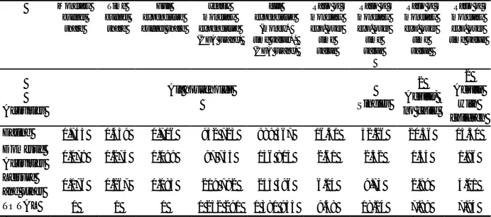
The descriptive statistics (see Table 1) suggests that the bulk of the household budget is spent on consumption. An examination of the structure of the household budget shows that on average 74.5% of the monetary budget is devoted to consumption, while 17.6% is allocated to leisure and other activities, and 7.9% for domestic activities. We have the same structure of household spending, taking into account the time budget; however with a lesser amplitude: 71.6% of the total budget is devoted to food, compared with 18.5% to leisure and other and 9.9% to domestic activities.
On average, households spend 1 252 291 CFA Franc on food, education, healthcare, transportation, housing, durable goods, leisure, and other items annually. Households have on average eleven members; 5.4% among family heads are female. Household heads are predominantly farmers (86%) most of them being 36–60 years old, and few exceeding 61. Only 14% of households attended school (see Table B1 in Appendix B).
Table 1: Money, time and full expenditure patterns (singles and couples)
Monetary budget share Time budget share Full expenditure budget share yearly monetary expenditure (CFA Franc) full expenditure (money+ time value*) (CFA Franc) Ratio of monetary exp. over time value Ratio of monetary exp. over time value Ratio of monetary exp. over time value Ratio of monetary exp. over time value Activities All households Singles 2 Adults, no child 2 Adults with children Eating 0.745 0.459 0.716 932 723 989 567 16.41 52.26 20.36 15.30 Domestic Activities 0.079 0.274 0.099 97 755 136 803 2.60 2.32 1.54 1.96 Leisure and other 0.176 0.267 0.185 219 792 255 586 6.14 9.73 2.99 4.01 TOTAL 1 1 1 1 252 291 1 381 955 9.58 18.14 7.89 7.94
*valuation of time expenditures by the estimated opportunity cost of time at the individual level.
The first theoretical models on the demand of households made the postulate of the dichotomy between functions of production and consumption of households. The Almost Ideal Demand System (AIDS) models are similar and explain the household demand by economic and financial variables (income, price), but also socio-demographic (place of residence, household size, education level and gender of head of household etc.). This model served for instance as a basis for the study of the Ministry of Economic Forecasting and the Plan of Morocco in 2002, in the estimation of income elasticities of the demand by product or group of products of Moroccan households.
One of the limitations of these models, which emerged in the context of the ambivalence of households (both consumers and producers), led simultaneously to consider the consumption and production functions (unit model) in the analysis of households’
demand. In this sense, referring to Rwanda, Muller (1992) insisted on the need to take into account production decisions to analyze the demand functions of agricultural producers. However, this new approach is not without criticism. The fundamental limit to the unitary model remains the strong hypothesis of the indivisibility of the utility function of the household. Households are characterized by internal power relations that substantially modify their demands (Meignel, 1997). Doss (2006) shows for instance that women’s share of farmland significantly increase budget shares on food in Ghana. Hence the so-called collective models that take into account the heterogeneity of household members’ preferences.
Despite this theoretical evolution, on the empirical level, the first generation of models is the most used one because of its flexibility and simplicity in interpretation. Empirical studies, specifically in African countries, are quite diverse and take into account both the economic and social sectors. For instance, Ouédraogo (2006) studied the demand for energy wood respectively in the cities of Ouagadougou. Dieng and Fall, (2015) were interested in the demand for household life insurance through a panel within WAEMU countries. On the social level, Briand et al. (2009) analyze household water demand in Dakar. Nanfosso and Kasiwa (2013) focused on the demand for prenatal care in the Democratic Republic of Congo.
These studies consisted of estimating household demand or price and income elasticities for goods and services or identifying the determinants of household demand. However, studies also noted that there are significant differences in dietary patterns and food supply structures both across regions and within regions such as Africa (Fabiosa, 2011). These differences influence the relationship between income and food demand and thus the impact of alternative policy mechanisms in different areas. In the specific case of Burkina Faso, Savadogo and Brandt (1987) showed (based on a 1983 survey) that income and demographic factors played major roles in household consumption profiles in Ouagadougou, and more specifically that the consumption of the traditional food products declined as incomes rose.
However, these studies did not take into account the time spent by households on different activities. It is this void that this paper attempts to fill. Moreover, the methodology adopted in this research makes it possible to calculate the opportunity cost of time, the inequalities linked to the demand for different goods while respecting the theoretical corpus of the consumer and the producer.
4. Results
4.1. Estimate of the opportunity cost of time
Two methods have been used to estimate the opportunity cost of time 𝜔: first, the first Order Conditions (FOC) give a system of equations of monetary and time expenditures depending on 𝜔 and the coefficient 𝛾𝑖 of the direct utility (equation A6 in Appendix A). The
opportunity cost have been differentiated in this estimation according to the family structure (9 different types of family being considered according to the numbers of adults and children). The average of the estimates of the opportunity cost of time for the whole population is 16.86 CFA Franc (s.e.=5.71), which is smaller than the minimum wage rate for rural households
(175 CFA Franc) and the average wage rate (around 164 CFA Franc). Perhaps only a small proportion of adults in the family (or none) have an easy access to the labor market, which diminishes their opportunity to earn money by working outside the family, and thus depreciate their opportunity cost of time. There may be an important heterogeneity of households in regards to their situation on the labor market, which is reflected in the large variation of the estimates of this cost made for each individual (in the second method thereafter). The coefficients 𝛾𝑖 of the utility function (which measure the elasticities of the utility with respect to the quantities of commodities which are home produced) are all positive and close to the average budget shares of the three commodities: 𝛾1 = 0.66 for Eating (full budget share =0.72); 𝛾2 = 0.16 for Domestic Activities (full budget share =0.10); 𝛾3 = 0.19 for leisure and other activities (full budget share =0.18).
The second method is based on the ratio of the marginal utilities for time and money (equation A4) which depends on all expenditures (in money and time) and the coefficients αi, βi and γi of the utility and the domestic production functions. These coefficients and expenditures are known at the household level, which allows estimating the opportunity cost of time for each household. Its average over the whole population is coherent with the value estimated by equation (A6): 31.71 francs and its variation quite important across the population (coefficient of variation equal to 41.89). As expected, the opportunity cost of time is positive and increasing with monetary and full total expenditure (with an elasticity equal to 0.25) as well as with the proportion of children. Similar correlations have been found in relation to family size in France and the US (Gardes, 2016; Alpman and Gardes, 2016).
4.2. Elasticities of substitution between time and money
Hamermesh (2008) gave the first test concerning the substitutability of these two factors measured by the elasticity of substitution originally proposed by Hicks in 1932. With 𝑚𝑖 the
monetary expenditure and 𝑡𝑖 the time used to produce one unit of activity 𝑖 (for instance a lunch), this parameter is defined as
𝜕𝑙𝑛(𝑚𝑖
𝑡𝑖)
𝜕𝑙𝑛𝜔 , 𝜔 being the opportunity cost of time supposed to
measure the relative price of time and monetary expenditures (this relative price being equal to the ratio of the marginal productivities of the two factors). Hamermesh (2008) estimates using American data lies between 0.2 and 0.3 for food expenditures, which shows that some partial substitution exists for this expenditure: an increasing value of time tends to increase the monetary expenditure relatively to the time spent on the domestic production of meals. This analysis have been renewed by Canelas et al. (2014) who estimated the elasticity of substitution for two developed countries (Canada and France) and two Latin American countries (Ecuador and Guatemala). They found that the elasticity of substitution is negative for all activities and smaller for food than for other activities (housing, transport, clothing, personal care, leisure and other activities): for instance in Guatemala, the elasticity is -0.34 for food and -0.75 for all activities but food.
The model which is estimated follows a logarithmic specification:
ln (𝑡𝑖ℎ
with 𝜎𝑖 the elasticity of substitution for commodity 𝑖, 𝑚𝑖ℎ and 𝑡𝑖ℎthe monetary expenditure and time use on good 𝑖 by household ℎ respectively, 𝜔ℎ the estimated opportunity cost of time for household h and 𝑍ℎ a vector of the household’s socio-economic characteristics (family size, proportion of children, age of the head).
The system of three equations for all activities is estimated under the constraint of a similar elasticity 𝜎 and gives an estimate of -0.083 (s.e. 0.029) for the three activities, which shows a statistically significant but small level of substitution compared to Hamermesh (2008) and Canelas et al. (2014) results. This may be due to the fact that rural households in Burkina Faso cannot easily buy market goods (durables, electricity, kitchen arrangements or bottles of water) to diminish the time spent to obtain and prepare food or for other domestic activities.
4.3. Income and price-elasticities for semi-aggregated expenditures
In Table 2, the full price elasticities are estimated on full budget shares, full income and the definition of full prices using the opportunity cost estimated at the individual level (i.e. for each household).
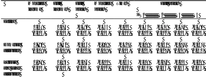
Table 2: Income, price and time elasticities Monetary income Full income* Full price* Monetary price*
Time* Full price*
Q1 Q2 Q3 Q4 Eating 1.039 (0.003) 0.073 (0.004) -0.492 (0.006) -0.445 (0.005) -0.026 (0.001) -0.442 (0.012) -0.509 (0.012) -0.470 (0.013) -0.491 (0.014) Domestic activities 0.791 (0.019) 0.752 (0.019) -1.146 (0.012) -0.819 (0.009) -0.327 (0.003) -1.118 (0.024) -1.160 (0.027) -1.177 (0.028) -1.167 (0.030) Leisure and other activities 0.878 (0.013) 0.884 (0.016) -1.176 (0.014) -1.011 (0.012) -0.165 (0.002) -1.119 (0.031) -1.272 (0.036) -1.203 (0.036) -1.228 (0.035)
Note : estimation with the specification of the AIDS on full expenditure. Individual estimate of the opportunity
cost of time. The monetary- and time-elasticities are obtained through a derivation of the full prices over these two components (see Gardes, 2016).
Q1, 2, 3, 4: quartiles of household’s income per unit of consumption (OECD equivalence scale).
Some important results come out of these estimations: first of all, we observe that all the (compensated) monetary own-price elasticities are significantly negative. The estimates are significantly larger in absolute value for domestic activities and leisure than those of the macroeconomics estimates that often oscillate around -0.5 for semi-aggregate commodities. As often pointed out, elasticities derived from macroeconomic data face measurement errors and aggregation which may bias their absolute values towards 0. Second, all elasticities with respect to time (in fact to time cost, i.e. time use 𝜏𝑖 multiplied by its opportunity cost) are
negative, and their magnitudes are unrelated with the income effect. Third, price and time elasticities change significantly according to the households well-being, measured by means of income per unit of consumption: price and time effects increase continuously with household income, being larger in absolute value by 20% for the fourth quartile of income compared to the first. The larger sensibility to prices observed for better-off families can be related to the notion that saturation of basic needs develops the possibility to substitute between activities when the relative prices change.
5. Price-elasticities for disaggregated expenditures
Micro-simulation exercises often require the calibration of income and price effect at a more precise level of the expenditures, for instance for alcoholic beverages when a specific tax is applied to them. This is possible under separability assumptions inside each broad activity (final good or commodity) such as food activity, as shown in Gardes (2014). The resulting formula for the price elasticities of expenditures on good 𝑖 pertaining to the semi-aggregate commodity 𝐼 is given as follow:
𝐸p∗ixi/pj = Epixi/pj𝐸PIXI/pI
𝐴 (2)
where Epixi/pj is the price elasticity calculated by the Frisch formula under the assumption of
strong separability in the semi-aggregate commodity 𝐼, 𝐸PIXI/pI the own-price elasticity of this semi-aggregate expenditure and A is the average of own and cross-price elasticities for all items in the final good 𝐼 weighted by the ratios of the corresponding budget shares, see equation (4) in Gardes, 2016). In order to calculate the price elasticity of the disaggregated expenditure 𝐼, we assume that individual expenditures are strongly separable within the aggregate 𝐼. This hypothesis allows to compute direct and cross-price elasticities following the Frisch formula:
𝐸𝑝𝑖𝑥𝑖/𝑝𝑗 = Ф𝐸𝑖𝛿𝑖𝑗− 𝐸𝑖𝑤𝑗(1 + Ф𝐸𝑗) (3)
where Ф is the Frisch income flexibility which is calibrated here at the value estimated in the literature: -0.5.
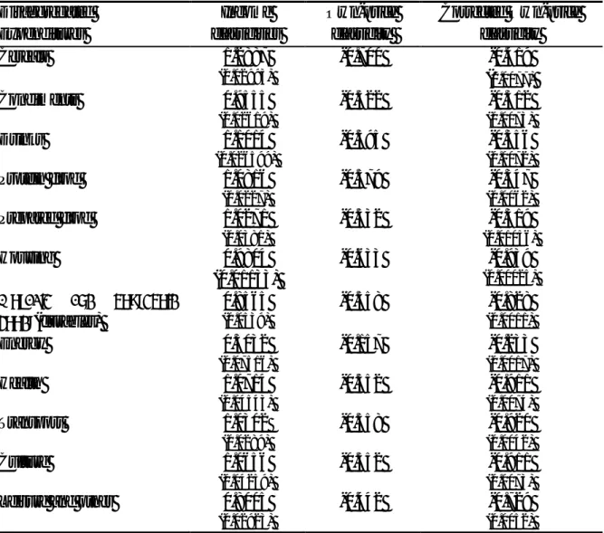
Table 3: Own-price elasticities for disaggregated expenditures: Burkina Faso Disaggregated Expenditures Income elasticities Own-price elasticity Corrected Own-price elasticity Cereals 1.2887 (0.02993) -0.700 -0.419 (0.0077) Condiments 0.9555 (0.02619) -0.522 -0.312 (0.0073) Drinks 1.1014 (0.026599) -0.595 -0.356 (0.0072) Protein food 1.0816 (0.0227) -0.579 -0.347 (0.0062) Prepared food 1.0271 (0.0381) -0.532 -0.319 (0.01056) Housing 0.9804 (0.01133) -0.633 -0.939 (0.00025)
Movable and household goods(durables) 0.8565 (0.0539) -0.558 -0.828 (0.0011) Energy 0.3032 (0.07516) -0.157 -0.233 (0.0017) Health 1.0714 (0.04543) -0.552 -0.911 (0.0074) Transport 1.0302 (0.0289) -0.558 -0.920 (0.0042) Culture 1.0656 (0.04259) -0.552 -0.911 (0.0073)
Leisure and other 0.8005
(0.02923)
-0.442 -0.729
(0.0052)
Note: Own-price elasticities are calculated using Frisch’s formula under strong separability assumption. The
inverse of the income flexibility Ф=𝜔ˇ−1 is set to the average value proposed by Frisch: -0.5 (see a discussion in Gardes, 2014). Income elasticities used in this formula have been estimated as within estimates on a panel dataset in order to correct for usual biases on income elasticities estimated in the cross-section dimension (Gardes et al., 2005). Correction of own-price elasticities by equation (3). Bootstrapped standard errors. Table 3 describes the sensitivity of demand to changes in income and prices. All these variables have a significant effect on demand. They have the expected effects according to economic theory. However, the magnitude of the positive effects of income on demand is greater than that of the negative effects of prices. As expected, the descriptive results indicate that food demand is more responsive to changes in income (income elasticities are higher) for cereals, drinks, compared to condiments that tend to constitute basic diets.
In line with the earlier literature (Bouis and Haddad, 1992), the use of cross-sectional data tends to result in higher elasticities. The use of household expenditures as a proxy for income generally results in lower income elasticities, which corresponds to the findings by Ogundari and Abdulai (2013) and Zhou and Yu (2015) and may relate to the fact that total expenditure is considered a more reliable proxy than reported income (Deaton, 1997). The use of a
demand system tends to provide higher income elasticities than single equation estimates, which confirms the findings of Zhou and Yu (2015).
6. Inequality based on full income
When a household is supposed to be able to substitute domestic production to the purchase of the corresponding markets goods or services, the sum of its consumptions and the total value of its domestic productions measure its full income. In order to obtain a well-being measure, this full income must be divided by an equivalence scale estimated for full expenditures. Inequality measured for full income per unit of consumption may thus differ from inequality obtained using households’ total monetary income because of the difference between the distributions of monetary and full income, and because of the larger adult and children full costs compared to children monetary costs (Gardes and Starzec, 2017). That definition of full income supposes that all fractions of time devoted to some activity by an adult of the household increases the household well-being by the corresponding monetary value indicated by the opportunity cost of time. Thus, the choice of that opportunity cost is crucial.
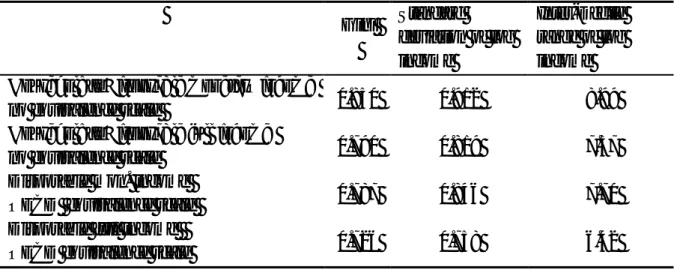
Results reported in table 4 show that both effects – measuring full income instead of monetary income and taking into account the cost of adults and children - diminish the inequality between households’ income by 7.4% on average according to the indicator for total income and 10.1% for income per consumption unit. The reduction of inequality is even larger when considering extreme income groups (Inter-Decile range of log income): it decreases by 20.9% for total income and 24.3% for income per U.C. between the first and the last decile of their distributions.
It is interesting to note that these results are similar to those obtained for developed countries such as France and the US (Gardes and Starzec, 2017; Alpman et al., 2016).
Table 4: Inequality indexes compared for monetary and full incomes
Gini Standard deviation of log income Inter-Decile range of log income Household’s Disposable monetary income
no equivalence scale 0.850 0.912 8.99
Household’s Disposable full income
no equivalence scale 0.790 0.819 7.57
Disposable mon. income
OECD equivalence scale 0.787 0.846 7.70
Disposable full income
7. Conclusion
This article uses Becker’s approach to analyze household consumption behavior taking into consideration their monetary income and their time value allocated to their activities.
Becker’s model of domestic production and allocation of time proves convenient to define a new method of estimation for the opportunity cost of time. The parameters of the (Cobb-Douglas) domestic production functions and utility are estimated locally (i.e. for each household), so that they correspond to local substitutions for the corresponding household. The constancy of the coefficients in the Cobb-Douglas specifications thus applies only in a small neighbourhood for the corresponding household.
This model provides precise and quite realistic price elasticities, which compare well with other estimation techniques applied to cross-section data. Thus, the ratios of full expenditures over the monetary seem to be good proxies for measuring the scarcity of commodities. Moreover, it allows the elasticities over time use to be computed. Micro-simulation exercises need often to calibrate income and price effect at a more precise level of the expenditures, for instance for alcoholic beverages when a specific tax is applied. This is possible under separability assumptions inside the broad group of commodities considered as activities in our analysis.
We estimated the monetary income and full income elasticities as well as the direct and cross prices of the 3 aggregate positions. Using an appropriate methodology, we were able to calculate the same elasticities for disaggregated positions. At the end, we have shown that economies of scale in the consumption of goods and services linked to large households in Burkina Faso make it possible to reduce inequalities by taking into account the value of time allocated to different activities. As a result, the paper leads to the calculation of a low opportunity cost of time, but in line with the economic theory and the results found in the developed countries. This weakness is explained by a weak rural SMIC and possibly by low substitution possibilities between market goods and services and time in rural areas.
The considerable differences in household expenditures across income level suggest that the impact of food and inequality reduction policy in Burkina Faso is likely to differ by categories of household.
Acknowledgements
The authors thank the General Directorate for the Promotion of the Rural Economy (DGPER) and the University of Ouaga II for data and the financing of the study trip of Thiombiano in Paris. In addition, they thank colleagues from the University of Paris I and those of Burkina Faso for their comments which enrich this paper.
References
Aguiar M.A., and Hurst E. (2007) "Measuring Trends in Leisure: the Allocation of Time over Five Decades", Quarterly Journal of Economic, 22 (3): 969-1006.
Alpman, A., and Gardes F. (2015) "Time-use during the Great recession – a Comment", w.p.
CES, 2015.12, PSE, University Paris I.
Alpman, A., and Gardes F. (2016) "A new method to estimate price and time elasticities on microdata: an application on US data", w.p. CES,PSE, University Paris I.
Alpman A., Gardes F. and S. Salazar S. (2016) "Income Inequality with Domestic Production", w.p. CES,PSE, University Paris I.
Becker G.S. (1965) "A Theory of the Allocation of Time", The Economic Journal, 75: 493- 517.
Becker G.S., and Michael R.T. (1973) "On the New Theory of Consumer Behavior", Swedish
Journal of Economics, 75 (4): 378-396.
Bouis H.E., and Haddad L.J. (1992) "Are estimates of calorie-income elasticities too high? A recalibration of the plausible range", Journal of Development Economics, 39 (2): 333- 364.
Briand B., Nauges C., et Travers M., (2009) "Les déterminants du choix d’approvisionnement en eau des ménages de Dakar", Revue d'économie du développement, 3 : 83-108
Canelas C., Gardes F., Merrigan P. and Salazar, S. (2014) "The Elasticity of Substitution between Time and Monetary Expenditures: an Estimation for Canada, Ecuador, France and Guatemala." w.p. CES 2014.71, PSE, University Paris I.
Capéau B., Dercon S., (2006) "Prices, Unit Values and Local Measurement Units in Rural Surveys: an Econometric Approach with an pplication to Poverty measurement in Ethiopia", Journal of African Economies, 15 (2): 881-211.
Deaton A. (1988) "Quality, Quantity, and Spatial Variation of Prices", American Economic
Review,78 (3): 418-430.
De Vany A., (1973) "The Revealed Value of Time in Air Travel", Review of Economics and
Statistics, February, 56 (1): 77-82.
Dieng M. S., et Fall M., (2015), "Les déterminants de la demande d’assurance vie : le cas de l’UEMOA", Revue d’Economie Théorique et Appliquée, 5(1) : 15-36.
Direction de la statistique, (2002), "Elasticités-Revenu de la demande des ménages",
Ministère de la Prévision Economique et du Plan, Royaume du Maroc, Dépôt Légal : 2002/1178 ; ISBN : 9981-20-190-1.
Doss C., 2006, The Effect of Intrhousehold Property Ownership on Expenditure Patterns in Ghana, Journal of African Economies, 15 (1): 149-180.
Handbook of The Economics of Food Consumption and Politics. Ed Lusk, Roosen and
Shorgren. Oxford Uiversity Press. ISBN 0199681325.
Gardes F., Duncan G. J., Gaubert P., Gurgand M., and Starzec C. (2005) "Panel and Pseudo-Panel Estimation of Cross-Sectional and Time Series Elasticities of Food Consumption: The Case of U.S. and Polish Data", Journal of Business & Economic
Statistics, 23 (2): 242-253.
Gardes F. (2014) "Full price elasticities and the opportunity cost for time: a Tribute to the Beckerian model of the allocation of time", w.p. CES n° 2014-14, PSE, University
Paris I.
Gardes F., (2016), "The estimation of price elasticities and the value of time in a domestic framework: an application on French micro-data", under revision in Annals of
Economics and Statistics.
Gardes, F. (2017) Price elasticities for Disaggregated Expenditures, w.p. PSE/University Paris
I.
Gardes F, Duncan G.J., Gaubert P., Gurgand M.and Starzec C. (2005) "A Comparison of Consumption Laws Estimated on American and Polish Panel and Pseudo-Panel Data", Journal of Business and Economic Statisistics 23: 242-253.
Gardes F., and Margolis D. (2015) "Labor Supply, Consumption and Domestic Production",
w.p. PSE/University Paris I.
Gardes F., and Starzec, C. (2017) "A Restatement of Equivalence Scales Using Time and Monetary Expenditures Combined with Individual Prices", to appear in the Review of
Income and Wealth.
Gronau R. (1977) "Leisure, Home Production, and Work – The theory of the Allocation of Time revisited", Journal of Political Economy, 85: 1099-1123.
Hamermesh D. S. (2008) "Direct Estimates of Household Production." Economics Letters, 98(1):31-34.
Meignel S. (1997) "Ménages, crise et bien-être dans les pays en développement : quelques enseignements de la littérature récente", Document de travail, Centre d’économie du
développement, Université Montesquieu-Bordeaux IV – France.
Muller C. (1992) "Estimation des consommations de producteurs agricoles d'Afrique centrale", Economie et Prévision, n°105, 4, pp.17-34.
Nanfosso R. T., et Kasiwa J. M. (2013) "Les déterminants de la demande de soins prénataux en République démocratique du Congo : Approche par données de comptage", African
Evaluation Journal, aejonline.org.
Ogundari K. and Abdulai, A. (2013) "Examining the Heterogeneity in Calorie–Income Elasticities: A Meta-Analysis.", Food Policy, 40, 119-128.
Ouédraogo B. (2006) "La demande de bois-énergie à Ouagadougou : esquisse d’évaluation de l’impact physique et des échecs des politiques de prix", Développement durable et
territoires. URL : http://developpementdurable.revues.org/4151 ; DOI :
10.4000/developpementdurable.4151.
Savadogo K. and Brandt, J.A. (1988) "Household Food Demand in Burkina Faso: Implications for Food Policy", Agricultural Economics, 2: 345-364
Zhou D. and Yu X. (2014) Calorie Elasticities with Income Dynamics: Evidence from the Literature. Global Food Discussion papers, No. 35.
Appendix A
The model of domestic production (Gardes, 2014, 2016)
The direct utility U depends on the consumption of final goods in quantities 𝑧𝑖 which are produced by the household using market goods and time. The domestic production functions are specified in terms of the monetary expenditures used to buy the market goods and the time used for the activity. Cobb Douglas specifications for the utility and the domestic production functions are chosen in order to allow the calculation of the opportunity cost of time as the ratio of the marginal utilities of total monetary expenditures and time use. Note that all the parameters of these two functions are estimated locally (i.e. for each household in the dataset). The optimization program is (all variables correspond to a household h which index is omitted in the equations):
max 𝑚𝑖,𝑡𝑖 𝑢(𝑍) = ∏ 𝑎𝑖𝑧𝑖𝛾𝑖 𝑖 𝑤𝑖𝑡ℎ 𝑧𝑖 = 𝑏𝑖𝑚𝑖 𝛼𝑖𝑡 𝑖 𝛽𝑖 (A1)
under the full income constraint:
∑ (𝑚𝑖 𝑖 + 𝜔𝑡𝑖) = 𝑤𝑡𝑤 + 𝜔(𝑇 − 𝑡𝑤) + 𝑉 (A2)
With 𝑡𝑤 the market labor time, 𝜔 the valuation of time in the domestic production 𝑇 − 𝑡𝑤 =
∑ 𝑡𝑖 𝑖 = 𝑇𝑑, 𝑤 the wage rate, 𝑤𝑡𝑤the household’s wage and 𝑉 other monetary incomes. Note
that the opportunity cost of time 𝜔 may differ from the market wage 𝑤 whenever there exist some imperfection on the labor market or if the disutility of labor is smaller for domestic production.
In order to estimate the opportunity cost of time, the utility function is re-written:
𝑢(𝑍𝑖) = ∏ 𝑎𝑖𝑍𝑖𝛾𝑖 𝑖 = ∏ 𝑎𝑖 𝑖𝑏𝑖[∏ 𝑚𝑖 𝛼𝑖𝛾𝑖 ∑ 𝛼𝑖𝛾𝑖 𝑖 ] ∑ 𝛼𝑖𝛾𝑖 [∏ 𝑡𝑖 𝛽𝑖𝛾𝑖 ∑ 𝛽𝑖𝛾𝑖 𝑖 ] ∑ 𝛽𝑖𝛾𝑖 = 𝑎𝑚′ ∑ 𝛼𝑖𝛾𝑖𝑡′ ∑ 𝛽𝑖𝛾𝑖 (A3)
with 𝑚′ and 𝑡′ the geometric weighted means of the monetary and time inputs with weights
𝛼𝑖𝛾𝑖
∑ 𝛼𝑖𝛾𝑖 and
𝛽𝑖𝛾𝑖
∑ 𝛽𝑖𝛾𝑖. Deriving the utility over income 𝑌 and total leisure and domestic production
time 𝑇𝑑 gives the opportunity cost of time :
𝜔 = 𝜕𝑢 𝜕𝑇𝑑 𝜕𝑢 𝜕𝑌 = 𝜕𝑢 𝜕𝑡′ 𝜕𝑡′ 𝜕𝑇𝑑 𝜕𝑢 𝜕𝑚′ 𝜕𝑚′ 𝜕𝑌 = 𝑚′ ∑ 𝛽𝑖𝛾𝑖 𝑡′ ∑ 𝛼𝑖𝛾𝑖 𝜕𝑡′ 𝜕𝑇𝑑 𝜕𝑚′ 𝜕𝑌 = ∑ 𝛽𝑖𝛾𝑖 ∑ 𝛼𝑖𝛾𝑖 𝑇𝑑𝐸𝑙𝑡′/𝑇𝑑 𝑌𝐸𝑙𝑚′/𝑌 (A4)
In order to calculate the parameters of the utility and domestic production functions, we consider the substitutions which are possible, first between time and money resources for the production of some activity, second between money expenditures (or equivalently time expenditures) concerning two different activities. These substitutions generate first order conditions which imply:
𝛼𝑖 =
𝑚𝑖
𝜔𝑡𝑖+𝑚𝑖, 𝛽𝑖 =
𝜔𝑡𝑖𝑖
𝜔𝑡𝑖+𝑚𝑖 (A5)
and the system of equations:
𝑚𝑖𝛾𝑗 = 𝑚𝑗𝛾𝑖 + 𝜔𝛾𝑖𝑡𝑗− 𝜔𝛾𝑗𝑡𝑖 (A6) This system of 𝑛(𝑛−1)
2 independent equations is estimated under the homogeneity constraint of
the utility function: ∑𝛾𝑖 = 1. In this system, the opportunity cost of time is over-identified, as well as all 𝛾𝑗. The resulting estimates of the opportunity cost of time 𝜔 and the parameters 𝛾𝑗
of the utility function are then used through equations (A5) to calculate αI and βI for each household. Finally, these estimates of parameters α, β and γ are used to estimate the opportunity cost of time 𝜔ℎ for each household in the population by equation (A4). The
average value of this parameter is used in a second step to re-calculate a second vector of 𝜔ℎ and the process is renewed till convergence. We use in this paper the estimate of 𝜔ℎ at the household level obtained by equation (A4) calibrating a first estimate of this opportunity cost by the level estimated in the system of equations (A6). These individual values of 𝜔ℎ are finally used to value time and calculate the full expenditures and the proxies to full prices.
Empirical definition of proxies of the full prices
Becker’s full price can be written: 𝐩𝐢𝐡𝐭𝐟 = 𝐩
𝐢𝐭+ 𝛚𝐡𝐭𝛕𝐢𝐡 with 𝝉𝒊𝒉 the time use necessary
to produce one unit of the activity i. Suppose that a Leontief technology allows the quantities of the two factors to be proportional to the activity:
𝐱𝐢𝐡𝐭= 𝛏𝐢𝐡𝐳𝐢𝐡𝐭 𝐚𝐧𝐝 𝐭𝐢𝐡𝐭= 𝛉𝐢𝐡𝐳𝐢𝐡𝐭, so that: 𝐭𝐢𝐡𝐭 = 𝛕𝐢𝐡𝒙𝐢𝐡𝐭 with 𝝉𝒊𝒉 =𝜽𝒊𝒉
𝝃𝒊𝒉
This case corresponds to an assumption of complementarity between the two factors in the domestic technology, which allows to calculate a proxy for the full price of activity i by the ratio of full expenditure over its monetary component:
πiht = (𝐩𝐢𝐭+𝛚𝐡𝐭𝛕𝐢𝐡𝐭)𝐱𝐢𝐡𝐭 𝐩𝐢𝐭𝐱𝐢𝐡𝐭 = 𝐩𝐢𝐭+𝛚𝐡𝐭𝛕𝐢𝐡𝐭 𝐩𝐢𝐭 = 𝟏 + 𝛚𝐡𝐭𝛕𝐢𝐡𝐭 𝐩𝐢𝐭 = 𝟏 𝐩𝐢𝐭𝐩𝐢𝐡𝐭 𝐟 (𝑨𝟕)
Note that under the assumption of a common monetary price pi for all households in a
between households deriving from their opportunity cost of time 𝝎𝒉 and the coefficient of production 𝝉𝒊𝒉. If the monetary price p changes between households or periods, the full price can be computed as the product of this proxy πih with piht: 𝐩𝐢𝐡𝐭𝐟 = 𝐩𝐢𝐡𝐭𝛑𝐢𝐡. With these
definitions, it is possible to measure the full prices, observing only monetary and full expenditures.
Another definition of full prices under the hypothesis of a complete substitution between the two factors is discussed in Alpman and Gardes (2016). The logarithmic of these two full prices differ only by 𝜷𝒊𝐥𝐨𝐠𝒎𝒊𝒉𝒕
𝒕𝒊𝒉 . We choose to estimate the demand system using the
proxies of the full prices under the complementary factors hypothesis because these proxies do not depend on the estimates of parameters 𝜷𝒊, and are supposed to be more robust estimates of the full prices.
Appendix B Descriptive Analysis
Table B1: Household sample and the head of household characteristics
Household sample characteristics Characteristics of the head of household
Number of households 6 941 Household size 11.06 N. adult 5.36 Size distribution (en %)
1-5 persons 16.77 6-8 persons 25.76 9-11 persons 20.64 12-15 persons 17.14 16 and more 19.68 Characteristics Percentage Age distribution (%)
Less than 35 years 21.4 36–60 years 55,8 61+ 22,8 Education (%) Not literate 78.94 No formal education 7.03 Primary 7.35 Rural School 2.39 Koranic 2.16 High school 2.02 College 0.11 Marital status (%) Single 3.54 Married 90.42 Widowed 4.45 Divorced 0.84 Free union 0.75